Engineering Materials Vol II (microstructures_ processing_ design) 2nd ed. - M. Ashby_ D. Jones (1999) WW Part 11 pot
Bạn đang xem bản rút gọn của tài liệu. Xem và tải ngay bản đầy đủ của tài liệu tại đây (861.02 KB, 27 trang )
Production, forming and joining of polymers 261
opened out flat, and rolled onto a drum. The properties normal to the surface of the
stretched film, or across the axis of the oriented fibre, are worse than before, but they
are never loaded in this direction so it does not matter. Here people emulate nature:
most natural polymers (wood, wool, cotton, silk) are highly oriented in just this way.
Joining of polymers
Polymers are joined by cementing, by welding and by various sorts of fasteners, many
themselves moulded from polymers. Joining, of course, can sometimes be avoided by
integral design, in which coupled components are moulded into a single unit.
A polymer is joined to itself by cementing with a solution of the same polymer in a
volatile solvent. The solvent softens the surfaces, and the dissolved polymer molecules
bond them together. Components can be joined by monomer-cementing: the surfaces are
coated with monomer which polymerises onto the pre-existing polymer chains, creating
a bond.
Polymers can be stuck to other materials with adhesives, usually epoxies. They can be
attached by a variety of fasteners, which must be designed to distribute the fastening
load uniformly over a larger area than is usual for metals, to avoid fracture. Ingenious
splined or split fasteners can be moulded onto polymer components, allowing the
parts to be snapped together; and threads can be moulded onto parts to allow them to
be screwed together. Finally, polymers can be friction-welded to bring the parts, rotating
or oscillating, into contact; frictional heat melts the surfaces which are held under
static load until they resolidify.
Further reading
E. C. Bahardt, Computer-aided Engineering for Injection Moulding, Hanser, 1983.
F. W. Billmeyer, Textbook of Polymer Science, 3rd edition, Wiley Interscience, 1984.
J. A. Brydson, Plastics Materials, 6th edition, Butterworth-Heinemann, 1996.
International Saechtling, Plastics Handbook, Hanser, 1983.
P. C. Powell and A. J. Ingen Housz, Engineering with Polymers, 2nd edition, Chapman and Hall,
1998.
A. Whelan, Injection Moulding Materials, Applied Science Publishers, 1982.
Problems
24.1 Describe in a few words, with an example or sketch where appropriate, what is
meant by each of the following:
(a) an addition reaction;
(b) a condensation reaction;
(c) a copolymer;
(d) a block copolymer;
(e) a plasticiser;
262 Engineering Materials 2
(f) a toughened polymer;
(g) a filler.
24.2 What forming process would you use to manufacture each of the following items;
(a) a continuous rod of PTFE;
(b) thin polyethylene film;
(c) a PMMA protractor;
(d) a ureaformaldehyde electrical switch cover;
(e) a fibre for a nylon rope.
24.3 Low-density polyethylene is being extruded at 200°C under a pressure of 60 MPa.
What increase in temperature would be needed to decrease the extrusion pressure
to 40 MPa? The shear rate is the same in both cases. [Hint: use eqns (23.13) and
(23.14) with C
1
= 17.5, C
2
= 52 K and T
0
= T
g
= 270 K.]
Answer: 32°C.
24.4 Discuss the problems involved in replacing the metal parts of an ordinary bicycle
with components made from polymers. Illustrate your answer by specific reference
to the frame, wheels, transmission and bearings.
Composites: fibrous, particulate and foamed 263
Chapter 25
Composites: fibrous, particulate and foamed
Introduction
The word “composites” has a modern ring. But using the high strength of fibres to
stiffen and strengthen a cheap matrix material is probably older than the wheel. The
Processional Way in ancient Babylon, one of the lesser wonders of the ancient world, was
made of bitumen reinforced with plaited straw. Straw and horse hair have been used
to reinforce mud bricks (improving their fracture toughness) for at least 5000 years.
Paper is a composite; so is concrete: both were known to the Romans. And almost all
natural materials which must bear load – wood, bone, muscle – are composites.
The composite industry, however, is new. It has grown rapidly in the past 30 years
with the development of fibrous composites: to begin with, glass-fibre reinforced polymers
(GFRP or fibreglass) and, more recently, carbon-fibre reinforced polymers (CFRP). Their
use in boats, and their increasing replacement of metals in aircraft and ground transport
systems, is a revolution in material usage which is still accelerating.
Composites need not be made of fibres. Plywood is a lamellar composite, giving a
material with uniform properties in the plane of the sheet (unlike the wood from
which it is made). Sheets of GFRP or of CFRP are laminated together, for the same
reason. And sandwich panels – composites made of stiff skins with a low-density core
– achieve special properties by combining, in a sheet, the best features of two very
different components.
Cheapest of all are the particulate composites. Aggregate plus cement gives concrete,
and the composite is cheaper (per unit volume) than the cement itself. Polymers can
be filled with sand, silica flour, or glass particles, increasing the stiffness and wear-
resistance, and often reducing the price. And one particulate composite, tungsten-
carbide particles in cobalt (known as “cemented carbide” or “hard metal”), is the basis
of the heavy-duty cutting tool industry.
But high stiffness is not always what you want. Cushions, packaging and crash-
padding require materials with moduli that are lower than those of any solid. This can
be done with foams – composites of a solid and a gas – which have properties which
can be tailored, with great precision, to match the engineering need.
We now examine the properties of fibrous and particulate composites and foams in
a little more detail. With these materials, more than any other, properties can be
designed-in; the characteristics of the material itself can be engineered.
Fibrous composites
Polymers have a low stiffness, and (in the right range of temperature) are ductile.
Ceramics and glasses are stiff and strong, but are catastrophically brittle. In fibrous
264 Engineering Materials 2
composites we exploit the great strength of the ceramic while avoiding the catastrophe:
the brittle failure of fibres leads to a progressive, not a sudden, failure.
If the fibres of a composite are aligned along the loading direction, then the stiffness
and the strength are, roughly speaking, an average of those of the matrix and fibres,
weighted by their volume fractions. But not all composite properties are just a linear
combination of those of the components. Their great attraction lies in the fact that,
frequently, something extra is gained.
The toughness is an example. If a crack simply ran through a GFRP composite, one
might (at first sight) expect the toughness to be a simple weighted average of that of
glass and epoxy; and both are low. But that is not what happens. The strong fibres pull
out of the epoxy. In pulling out, work is done and this work contributes to the tough-
ness of the composite. The toughness is greater – often much greater – than the linear
combination.
Polymer-matrix composites for aerospace and transport are made by laying up glass,
carbon or Kevlar fibres (Table 25.1) in an uncured mixture of resin and hardener. The
resin cures, taking up the shape of the mould and bonding to the fibres. Many com-
posites are based on epoxies, though there is now a trend to using the cheaper polyesters.
Laying-up is a slow, labour-intensive job. It can be by-passed by using thermoplast-
ics containing chopped fibres which can be injection moulded. The random chopped
fibres are not quite as effective as laid-up continuous fibres, which can be oriented to
maximise their contribution to the strength. But the flow pattern in injection moulding
helps to line the fibres up, so that clever mould design can give a stiff, strong product.
The technique is used increasingly for sports goods (tennis racquets, for instance) and
light-weight hiking gear (like back-pack frames).
Making good fibre-composites is not easy; large companies have been bankrupted
by their failure to do so. The technology is better understood than it used to be; the
tricks can be found in the books listed under Further reading. But suppose you can
make them, you still have to know how to use them. That needs an understanding of
their properties, which we examine next. The important properties of three common
composites are listed in Table 25.2, where they are compared with a high-strength steel
and a high-strength aluminium alloy of the sort used for aircraft structures.
Table 25.1 Properties of some fibres and matrices
Material Density
r
(Mg m
−
3
) Modulus
E
(GPa) Strength
s
f
(MPa)
Fibres
Carbon, Type1 1.95 390 2200
Carbon, Type2 1.75 250 2700
Cellulose fibres 1.61 60 1200
Glass (E-glass) 2.56 76 1400–2500
Kevlar 1.45 125 2760
Matrices
Epoxies 1.2–1.4 2.1–5.5 40–85
Polyesters 1.1–1.4 1.3–4.5 45–85
Composites: fibrous, particulate and foamed 265
Table 25.2 Properties, and specific properties, of composites
Material Density
r
Young’s Strength Fracture
E/r E
1/2
/r E
1/3
/rs
y
/r
(Mg m
−
3
) modulus
s
y
(MPa) toughness
E
(GPa)
K
IC
(MPa m
1/2
)
Composites
CFRP, 58% uniaxial C in epoxy 1.5 189 1050 32–45 126 9 3.8 700
GFRP, 50% uniaxial glass in polyester 2.0 48 1240 42–60 24 3.5 1.8 620
Kevlar-epoxy (KFRP), 60% uniaxial 1.4 76 1240 – 54 6.2 3.0 886
Kevlar in epoxy
Metals
High-strength steel 7.8 207 1000 100 27 1.8 0.76 128
Aluminium alloy 2.8 71 500 28 25 3.0 1.5 179
266 Engineering Materials 2
Fig. 25.1. (a) When loaded along the fibre direction the fibres and matrix of a continuous-fibre composite
suffer equal strains. (b) When loaded across the fibre direction, the fibres and matrix see roughly equal
stress; particulate composites are the same. (c) A 0 –90° laminate has high and low modulus directions;
a 0– 45–90–135° laminate is nearly isotropic.
Modulus
When two linear-elastic materials (though with different moduli) are mixed, the
mixture is also linear-elastic. The modulus of a fibrous composite when loaded along
the fibre direction (Fig. 25.1a) is a linear combination of that of the fibres, E
f
, and the
matrix, E
m
E
c||
= V
f
E
f
+ (1 − V
f
)E
m
(25.1)
where V
f
is the volume fraction of fibres (see Book 1, Chapter 6). The modulus of the
same material, loaded across the fibres (Fig. 25.1b) is much less – it is only
E
V
E
V
E
c
f
f
f
m
⊥
−
=+
−
1
1
(25.2)
(see Book 1, Chapter 6 again).
Table 25.1 gives E
f
and E
m
for common composites. The moduli E
||
and E
⊥
for a
composite with, say, 50% of fibres, differ greatly: a uniaxial composite (one in which
all the fibres are aligned in one direction) is exceedingly anisotropic. By using a cross-
weave of fibres (Fig. 25.1c) the moduli in the 0 and 90° directions can be made equal,
but those at 45° are still very low. Approximate isotropy can be restored by laminating
sheets, rotated through 45°, to give a plywood-like fibre laminate.
Composites: fibrous, particulate and foamed 267
Fig. 25.2. The stress–strain curve of a continuous fibre composite (heavy line), showing how it relates to
those of the fibres and the matrix (thin lines). At the peak the fibres are on the point of failing.
Tensile strength and the critical fibre length
Many fibrous composites are made of strong, brittle fibres in a more ductile polymeric
matrix. Then the stress–strain curve looks like the heavy line in Fig. 25.2. The figure
largely explains itself. The stress–strain curve is linear, with slope E (eqn. 25.1) until the
matrix yields. From there on, most of the extra load is carried by the fibres which con-
tinue to stretch elastically until they fracture. When they do, the stress drops to the yield
strength of the matrix (though not as sharply as the figure shows because the fibres do
not all break at once). When the matrix fractures, the composite fails completely.
In any structural application it is the peak stress which matters. At the peak, the
fibres are just on the point of breaking and the matrix has yielded, so the stress is given
by the yield strength of the matrix,
σ
m
y
, and the fracture strength of the fibres,
σ
f
f
,
combined using a rule of mixtures
σ
TS
= V
f
σ
f
f
+ (1 − V
f
)
σ
m
y
. (25.3)
This is shown as the line rising to the right in Fig. 25.3. Once the fibres have fractured, the
strength rises to a second maximum determined by the fracture strength of the matrix
σ
TS
= (1 − V
f
)
σ
m
f
(25.4)
where
σ
m
f
is the fracture strength of the matrix; it is shown as the line falling to the
right on Fig. 25.3. The figure shows that adding too few fibres does more harm than
good: a critical volume fraction
V
f
crit
of fibres must be exceeded to give an increase in
strength. If there are too few, they fracture before the peak is reached and the ultimate
strength of the material is reduced.
For many applications (e.g. body pressings), it is inconvenient to use continuous
fibres. It is a remarkable feature of these materials that chopped fibre composites
(convenient for moulding operations) are nearly as strong as those with continuous
fibres, provided the fibre length exceeds a critical value.
Consider the peak stress that can be carried by a chopped-fibre composite which has
a matrix with a yield strength in shear of
σ
m
s
(
σ
m
s
≈
1
–
2
σ
m
y
). Figure 25.4 shows that the
axial force transmitted to a fibre of diameter d over a little segment
δ
x of its length is
δ
F =
π
d
σ
m
s
δ
x. (25.5)
268 Engineering Materials 2
Fig. 25.3. The variation of peak stress with volume fraction of fibres. A minimum volume fraction (
V
f
crit
) is
needed to give any strengthening.
Fig. 25.4. Load transfer from the matrix to the fibre causes the tensile stress in the fibre to rise to peak in the
middle. If the peak exceeds the fracture strength of the fibre, it breaks.
The force on the fibre thus increases from zero at its end to the value
Fdxdx
s
m
s
m
x
==
∫
πσ πσ
d
0
(25.6)
at a distance x from the end. The force which will just break the fibre is
F
d
c
f
f
.=
π
σ
2
4
(25.7)
Equating these two forces, we find that the fibre will break at a distance
x
d
c
f
f
s
m
=
4
σ
σ
(25.8)
from its end. If the fibre length is less than 2x
c
, the fibres do not break – but nor do
they carry as much load as they could. If they are much longer than 2x
c
, then nothing
is gained by the extra length. The optimum strength (and the most effective use of the
Composites: fibrous, particulate and foamed 269
Fig. 25.5. Composites fail in compression by kinking, at a load which is lower than that for failure in tension.
fibres) is obtained by chopping them to the length 2x
c
in the first place. The average
stress carried by a fibre is then simply
σ
f
f
/2 and the peak strength (by the argument
developed earlier) is
σ
σ
σ
TS
( ) .=+−
V
V
f
f
f
f
y
m
2
1
(25.9)
This is more than one-half of the strength of the continuous-fibre material (eqn. 25.3).
Or it is if all the fibres are aligned along the loading direction. That, of course, will not
be true in a chopped-fibre composite. In a car body, for instance, the fibres are ran-
domly oriented in the plane of the panel. Then only a fraction of them – about
1
4
– are
aligned so that much tensile force is transferred to them, and the contributions of the
fibres to the stiffness and strength are correspondingly reduced.
The compressive strength of composites is less than that in tension. This is because the
fibres buckle or, more precisely, they kink – a sort of co-operative buckling, shown in
Fig. 25.5. So while brittle ceramics are best in compression, composites are best in tension.
Toughness
The toughness G
c
of a composite (like that of any other material) is a measure of the energy
absorbed per unit crack area. If the crack simply propagated straight through the matrix
(toughness G
m
c
) and fibres (toughness G
f
c
), we might expect a simple rule-of-mixtures
G
c
= V
f
G
f
c
+ (1 − V
f
)G
m
c
. (25.10)
But it does not usually do this. We have already seen that, if the length of the fibres is
less than 2x
c
, they will not fracture. And if they do not fracture they must instead pull
out as the crack opens (Fig. 25.6). This gives a major new contribution to the tough-
ness. If the matrix shear strength is
σ
m
s
(as before), then the work done in pulling a fibre
out of the fracture surface is given approximately by
Fx d xx d
l
l
s
m
s
m
l
dd
/
==
∫∫
0
2
2
0
2
8
πσ πσ
ր
(25.11)
The number of fibres per unit crack area is 4V
f
/
π
d
2
(because the volume fraction is the
same as the area fraction on a plane perpendicular to the fibres). So the total work done
per unit crack area is
270 Engineering Materials 2
Fig. 25.6. Fibres toughen by pulling out of the fracture surface, absorbing energy as the crack opens.
Gd
l
V
d
V
d
l
cs
m
ff
s
m
.=×=
πσ
π
σ
2
2
2
8
4
2
(25.12)
This assumes that l is less than the critical length 2x
c
. If l is greater than 2x
c
the fibres
will not pull out, but will break instead. Thus optimum toughness is given by setting
l = 2x
c
in eqn. (25.12) to give
G
V
d
x
V
d
d
Vd
c
f
s
m
c
f
s
m
f
f
s
m
ff
f
s
m
()
.==
=
22
48
2
2
2
σσ
σ
σ
σ
σ
(25.13)
The equation says that, to get a high toughness, you should use strong fibres in a weak
matrix (though of course a weak matrix gives a low strength). This mechanism gives
CFRP and GFRP a toughness (50 kJ m
−2
) far higher than that of either the matrix (5 kJ m
−2
) or
the fibres (0.1 kJ m
−2
); without it neither would be useful as an engineering material.
Applications of composites
In designing transportation systems, weight is as important as strength. Figure 25.7
shows that, depending on the geometry of loading, the component which gives the
least deflection for a given weight is that made of a material with a maximum E/
ρ
(ties
in tension), E
1/2
/
ρ
(beam in bending) or E
1/3
/
ρ
(plate in bending).
When E/
ρ
is the important parameter, there is nothing to choose between steel,
aluminium or fibre glass (Table 25.2). But when E
1/2
/
ρ
is controlling, aluminium is
better than steel: that is why it is the principal airframe material. Fibreglass is not
Composites: fibrous, particulate and foamed 271
Fig. 25.7. The combination of properties which maximise the stiffness-to-weight ratio and the strength-to-
weight ratio, for various loading geometries.
significantly better. Only CFRP and KFRP offer a real advantage, and one that is now
exploited extensively in aircraft structures. This advantage persists when E
1/3
/
ρ
is the
determining quantity – and for this reason both CFRP and KFRP find particular applica-
tion in floor panels and large load-bearing surfaces like flaps and tail planes.
In some applications it is strength, not stiffness, that matters. Figure 25.7 shows that
the component with the greatest strength for a given weight is that made of the mater-
ial with a maximum
σ
y
/
ρ
(ties in tension),
σρ
y
23/
/
(beams in bending) or
σρ
y
12/
/
(plates in bending). Even when
σ
y
/
ρ
is the important parameter, composites are better
than metals (Table 25.2), and the advantage grows when
σρ
y
23/
/
or
σρ
y
12/
/
are dominant.
Despite the high cost of composites, the weight-saving they permit is so great that
their use in trains, trucks and even cars is now extensive. But, as this chapter illus-
trates, the engineer needs to understand the material and the way it will be loaded in
order to use composites effectively.
Particulate composites
Particulate composites are made by blending silica flour, glass beads, even sand into a
polymer during processing.
272 Engineering Materials 2
Particulate composites are much less efficient in the way the filler contributes to the
strength. There is a small gain in stiffness, and sometimes in strength and toughness,
but it is far less than in a fibrous composite. Their attraction lies more in their low cost
and in the good wear resistance that a hard filler can give. Road surfaces are a good
example: they are either macadam (a particulate composite of gravel in bitumen, a
polymer) or concrete (a composite of gravel in cement, for which see Chapter 20).
Cellular solids, or foams
Many natural materials are cellular: wood and bone, for example; cork and coral, for
instance. There are good reasons for this: cellular materials permit an optimisation of
stiffness, or strength, or of energy absorption, for a given weight of material. These
natural foams are widely used by people (wood for structures, cork for thermal insula-
tion), and synthetic foams are common too: cushions, padding, packaging, insulation,
are all functions filled by cellular polymers. Foams give a way of making solids which
are very light and, if combined with stiff skins to make sandwich panels, they give
structures which are exceptionally stiff and light. The engineering potential of foams is
considerable, and, at present, incompletely realised.
Most polymers can be foamed easily. It can be done by simple mechanical stirring or
by blowing a gas under pressure into the molten polymer. But by far the most useful
method is to mix a chemical blowing agent with the granules of polymer before pro-
cessing: it releases CO
2
during the heating cycle, generating gas bubbles in the final
moulding. Similar agents can be blended into thermosets so that gas is released during
curing, expanding the polymer into a foam; if it is contained in a closed mould it takes
up the mould shape accurately and with a smooth, dense, surface.
The properties of a foam are determined by the properties of the polymer, and by
the relative density,
ρ
/
ρ
s
: the density of the foam (
ρ
) divided by that of the solid (
ρ
s
) of
which it is made. This plays the role of the volume fraction V
f
of fibres in a composite,
and all the equations for foam properties contain
ρ
/
ρ
s
. It can vary widely, from 0.5 for
a dense foam to 0.005 for a particularly light one.
The cells in foams are polyhedral, like grains in a metal (Fig. 25.8). The cell walls,
where the solid is concentrated, can be open (like a sponge) or closed (like a flotation
foam), and they can be equiaxed (like the polymer foam in the figure) or elongated
Fig. 25.8. Polymeric foams, showing the polyhedral cells. Some foams have closed cells, others have cells
which are open.
Composites: fibrous, particulate and foamed 273
Fig. 25.9. The compressive stress–strain curve for a polymeric foam. Very large compressive strains are
possible, so the foam absorbs a lot of energy when it is crushed.
(like cells in wood). But the aspect of structures which is most important in determin-
ing properties is none of these; it is the relative density. We now examine how foam
properties depend on
ρ
/
ρ
s
and on the properties of the polymer of which it is made
(which we covered in Chapter 23).
Mechanical properties of foams
When a foam is compressed, the stress–strain curve shows three regions (Fig. 25.9). At
small strains the foam deforms in a linear-elastic way: there is then a plateau of deforma-
tion at almost constant stress; and finally there is a region of densification as the cell
walls crush together.
At small strains the cell walls at first bend, like little beams of modulus E
s
, built in at
both ends. Figure 25.10 shows how a hexagonal array of cells is distorted by this
bending. The deflection can be calculated from simple beam theory. From this we
obtain the stiffness of a unit cell, and thus the modulus E of the foam, in terms of the
length l and thickness t of the cell walls. But these are directly related to the relative
density:
ρ
/
ρ
s
= (t/l)
2
for open-cell foams, the commonest kind. Using this gives the
foam modulus as
EE
s
s
.=
ρ
ρ
2
(25.14)
Real foams are well described by this formula. Note that foaming offers a vast range of
modulus:
ρ
/
ρ
s
can be varied from 0.5 to 0.005, a factor of 10
2
, by processing, allowing
E to be varied over a factor of 10
4
.
Linear-elasticity, of course, is limited to small strains (5% or less). Elastomeric foams
can be compressed far more than this. The deformation is still recoverable (and thus
elastic) but is non-linear, giving the plateau on Fig. 25.9. It is caused by the elastic
274 Engineering Materials 2
Fig. 25.10. Cell wall bending gives the linear-elastic portion of the stress–strain curve.
buckling of the columns or plates which make up the cell edges or walls, as shown in
Fig. 25.11. Again using standard results of beam theory, the elastic collapse stress
σ
*
el
can
be calculated in terms of the density
ρ
. The result is
σ
*
el
=
005
2
E
s
s
ρ
ρ
(25.15)
As before, the strength of the foam is controlled by the density, and can be varied at
will through a wide range. Low-density (
ρ
/
ρ
s
= 0.01) elastomeric foams collapse under
tiny stresses; they are used to package small, delicate instruments. Denser foams (
ρ
/
ρ
s
= 0.05) are used for seating and beds: their moduli and collapse strengths are 25 times
larger. Still denser foams are used for packing heavier equipment: appliances or small
machine tools, for instance.
Fig. 25.11. When an elastomeric foam is compressed beyond the linear region, the cell walls buckle
elastically, giving the long plateau shown in Fig. 25.9.
Composites: fibrous, particulate and foamed 275
Fig. 25.12. When a plastic foam is compressed beyond the linear region, the cell walls bend plastically,
giving a long plateau exactly like that of Fig. 25.9.
Cellular materials can collapse by another mechanism. If the cell-wall material is
plastic (as many polymers are) then the foam as a whole shows plastic behaviour. The
stress–strain curve still looks like Fig. 25.9, but now the plateau is caused by plastic
collapse. Plastic collapse occurs when the moment exerted on the cell walls exceeds its
fully plastic moment, creating plastic hinges as shown in Fig. 25.12. Then the collapse
stress
σ
*
pl
of the foam is related to the yield strength
σ
y
of the wall by
σ
*
pl
=
/
03
32
σ
ρ
ρ
y
s
(25.16)
Plastic foams are good for the kind of packaging which is meant to absorb the energy
of a single impact: polyurethane automobile crash padding, polystyrene foam to protect
a television set if it is accidentally dropped during delivery. The long plateau of the
stress–strain curve absorbs energy but the foam is damaged in the process.
Materials that can be engineered
The materials described in this chapter differ from most others available to the
designer in that their properties can be engineered to suit, as nearly as possible, the
application. The stiffness, strength and toughness of a composite are, of course, con-
trolled by the type and volume fraction of fibres. But the materials engineering can go
further than this, by orienting or laminating the fibre weave to give directional proper-
ties, or to reinforce holes or fixing points, or to give a stiffness which varies in a
controlled way across a component. Foaming, too, allows new degrees of freedom to
the designer. Not only can the stiffness and strength be controlled over a vast range
(10
4
or more) by proper choice of matrix polymer and foam density, but gradients of
foam density and thus of properties can be designed-in. Because of this direct control
276 Engineering Materials 2
over properties, both sorts of composites offer special opportunities for designing
weight-optimal structures, particularly attractive in aerospace and transport. Examples
of this sort of design can be found in the books listed below.
Further reading
M. R. Piggott, Load Bearing Fibre Composites, Pergamon Press, 1980.
A. F. Johnson, Engineering Design Properties of GFRP, British Plastics Federation, 1974.
M. Grayson (editor), Encyclopedia of Composite Materials and Components, Wiley, 1983.
P. C. Powell and A. J. Ingen Housz, Engineering with Polymers, 2nd edition, Chapman and Hall,
1998.
L. J. Gibson and M. F. Ashby, Cellular Solids, 2nd edition, Butterworth-Heinemann, 1997.
D. Hull, An Introduction to Composite Materials, Cambridge University Press, 1981.
N. C. Hillyard (editor), Mechanics of Cellular Plastics, Applied Science Publishers, 1982.
Problems
25.1 A unidirectional fibre composite consists of 60% by volume of Kevlar fibres in a
matrix of epoxy. Find the moduli E
c||
and E
cЌ
. Comment on the accuracy of your
value for E
cЌ
. Use the moduli given in Table 25.1, and use an average value where
a range of moduli is given.
Answers: 77 GPa and 9 GPa.
25.2 A unidirectional fibre composite consists of 60% by volume of continuous type-1
carbon fibres in a matrix of epoxy. Find the maximum tensile strength of the
composite. You may assume that the matrix yields in tension at a stress of
40 MPa.
Answer: 1336 MPa.
25.3 A composite material for a car-repair kit consists of a random mixture of short
glass fibres in a polyester matrix. Estimate the maximum toughness G
c
of the
composite. You may assume that: the volume fraction of glass is 30%; the fibre
diameter is 15
µ
m; the fracture strength of the fibres is 1400 MPa; and the shear
strength of the matrix is 30 MPa.
Answer: 37 kJ m
–2
.
25.4 Calculate the critical length 2X
c
of the fibres in Problem 25.3. How would you
expect G
c
to change if the fibres were substantially longer than 2X
c
?
Answer: 0.35 mm.
Special topic: wood 277
Chapter 26
Special topic: wood
Introduction
Wood is the oldest and still most widely used of structural materials. Its documented
use in buildings and ships spans more than 5000 years. In the sixteenth century the
demand for stout oaks for ship-building was so great that the population of suitable
trees was seriously depleted, and in the seventeenth and eighteenth centuries much of
Europe was deforested completely by the exponential growth in consumption of wood.
Today the world production is about the same as that of iron and steel: roughly
10
9
tonnes per year. Much of this is used structurally: for beams, joists, flooring or
supports which will bear load. Then the properties which interest the designer are the
moduli, the yield or crushing strength, and the toughness. These properties, summarised
in Table 26.1, vary considerably: oak is about 5 times stiffer, stronger and tougher than
balsa, for instance. In this case study we examine the structure of wood and the way
the mechanical properties depend on it, using many of the ideas developed in the
preceding five chapters.
Table 26.1 Mechanical properties of woods
Wood Density
1
Young’s modulus
1,2
Strength
1,3
(MPa) Fracture toughness
1
(Mg m
−
3
) (GPa)
||
to grain (MPa m
1/2
)
||
to grain
⊥
to grain Tension Compression
||
to grain
⊥
to grain
Balsa 0.1–0.3 4 0.2 23 12 0.05 1.2
Mahogany 0.53 13.5 0.8 90 46 0.25 6.3
Douglas fir 0.55 16.4 1.1 70 42 0.34 6.2
Scots pine 0.55 16.3 0.8 89 47 0.35 6.1
Birch 0.62 16.3 0.9 – – 0.56 –
Ash 0.67 15.8 1.1 116 53 0.61 9.0
Oak 0.69 16.6 1.0 97 52 0.51 4.0
Beech 0.75 16.7 1.5 – – 0.95 8.9
1
Densities and properties of wood vary considerably; allow ±20% on the data shown here. All properties vary
with moisture content and temperature; see text.
2
Dynamic moduli; moduli in static tests are about two-thirds of these.
3
Anisotropy increases as the density decreases. The transverse strength is usually between 10% and 20% of the
longitudinal.
278 Engineering Materials 2
Fig. 26.1. The macrostructure of wood. Note the co-ordinate system (axial, radial, tangential).
The structure of wood
It is necessary to examine the structure of wood at three levels. At the macroscopic
(unmagnified) level the important features are shown in Fig. 26.1. The main cells
(“fibres” or “tracheids”) of the wood run axially up and down the tree: this is the
direction in which the strength is greatest. The wood is divided radially by the growth
rings: differences in density and cell size caused by rapid growth in the spring and
summer, and sluggish growth in the autumn and winter. Most of the growing pro-
cesses of the tree take place in the cambium, which is a thin layer just below the bark.
The rest of the wood is more or less dead; its function is mechanical: to hold the tree
up. With 10
8
years in which to optimise its structure, it is perhaps not surprising that
wood performs this function with remarkable efficiency.
To see how it does so, one has to examine the structure at the microscopic (light
microscope or scanning electron microscope) level. Figure 26.2 shows how the wood is
made up of long hollow cells, squeezed together like straws, most of them parallel to
the axis of the tree. The axial section shows roughly hexagonal cross-sections of the
cells: the radial and the tangential sections show their long, thin shape. The structure
appears complicated because of the fat tubular sap channels which run up the axis of
the tree carrying fluids from the roots to the branches, and the strings of smaller cells
called rays which run radially outwards from the centre of the tree to the bark. But
Special topic: wood 279
Fig. 26.2. The microstructure of wood. Woods are foams of relative densities between 0.07 and 0.5, with
cell walls which are fibre-reinforced. The properties are very anisotropic, partly because of the cell shape and
partly because the cell-wall fibres are aligned near the axial direction.
neither is of much importance mechanically; it is the fibres or tracheids which give
wood its stiffness, strength and toughness.
The walls of these tracheid cells have a structure at a molecular level, which (but for
the scale) is like a composite – like fibreglass, for example (Fig. 26.3). The role of the
strong glass fibres is taken by fibres of crystalline cellulose, a high polymer (C
6
H
10
O
5
)
n
,
made by the tree from glucose, C
6
H
12
O
6
, by a condensation reaction, and with a
DP
of
about 10
4
. Cellulose is a linear polymer with no cumbersome side-groups, so it crystal-
lises easily into microfibrils of great strength (these are the fibres you can sometimes see
in coarse paper). Cellulose microfibrils account for about 45% of the cell wall. The role
of the epoxy matrix is taken by the lignin, an amorphous polymer (like epoxy), and by
hemicellulose, a partly crystalline polymer of glucose with a smaller
DP
than cellulose;
between them they account for a further 40% of the weight of the wood. The remain-
ing 10–15% is water and extractives: oils and salts which give wood its colour, its smell,
and (in some instances) its resistance to beetles, bugs and bacteria. The chemistry of
wood is summarised in Table 26.2.
Fig. 26.3. The molecular structure of a cell wall. It is a fibre-reinforced composite (cellulose fibres in a matrix
of hemicellulose and lignin).
280 Engineering Materials 2
Table 26.2 Composition of cell wall of wood
Material Structure Approx. wt%
Fibres
Cellulose (C
6
H
10
O
5
)
n
Crystalline 45
Matrix
Lignin Amorphous 20
Hemicellulose Semi-crystalline 20
Water Dissolved in the matrix 10
Extractives Dispersed in the matrix 5
It is a remarkable fact that, although woods differ enormously in appearance, the
composition and structure of their cell walls do not. Woods as different as balsa and
beech have cell walls with a density
ρ
s
of 1.5 Mg m
−3
with the chemical make-up given
in Table 26.2 and with almost the same elaborate lay-up of cellulose fibres (Fig. 26.3).
The lay-up is important because it accounts, in part, for the enormous anisotropy of
wood – the difference in strength along and across the grain. The cell walls are helically
wound, like the handle of a CFRP golf club, with the fibre direction nearer the cell axis
rather than across it. This gives the cell wall a modulus and strength which are large
parallel to the axis of the cell and smaller (by a factor of about 3) across it. The
properties of the cell wall are summarised in Table 26.3; it is a little less stiff, but nearly
as strong as an aluminium alloy.
Wood, then, is a foamed fibrous composite. Both the foam cells and the cellulose
fibres in the cell wall are aligned predominantly along the grain of the wood (i.e.
parallel to the axis of the trunk). Not surprisingly, wood is mechanically very anisotropic:
the properties along the grain are quite different from those across it. But if all woods
are made of the same stuff, why do the properties range so widely from one sort of
wood to another? The differences between woods are primarily due to the differences
in their relative densities (see Table 26.1). This we now examine more closely.
The mechanical properties of wood
All the properties of wood depend to some extent on the amount of water it contains.
Green wood can contain up to 50% water. Seasoning (for 2 to 10 years) or kiln drying
(for a few days) reduces this to around 14%. The wood shrinks, and its modulus and
Table 26.3 Properties of cell wall
Property Axial Transverse
Density, r
s
(Mg m
−3
) 1.5
Modulus,
E
s
(GPa) 35 10
Yield strength, s
y
(MPa) 150 50
Special topic: wood 281
strength increase (because the cellulose fibrils pack more closely). To prevent move-
ment, wood should be dried to the value which is in equilibrium with the humidity
where it will be used. In a centrally heated house (20°C, 65% humidity), for example,
the equilibrium moisture content is 12%. Wood shows ordinary thermal expansion, of
course, but its magnitude (
α
= 5 MK
−1
along the grain, 50 MK
−1
across the grain) is
small compared to dimensional changes caused by drying.
Elasticity
Woods are visco-elastic solids: on loading they show an immediate elastic deformation
followed by a further slow creep or “delayed” elasticity. In design with wood it is
usually adequate to treat the material as elastic, taking a rather lower modulus for
long-term loading than for short loading times (a factor of 3 is realistic) to allow for the
creep. The modulus of a wood, for a given water content, then depends principally on
its density, and on the angle between the loading direction and the grain.
Figure 26.4 shows how Young’s modulus along the grain (“axial” loading) and across
the grain (“radial” or “tangential” loading) varies with density. The axial modulus varies
linearly with density and the others vary roughly as its square. This means that the
anisotropy of the wood (the ratio of the modulus along the grain to that across the grain)
increases as the density decreases: balsa woods are very anisotropic; oak or beech are
less so. In structural applications, wood is usually loaded along the grain: then only
the axial modulus is important. Occasionally it is loaded across the grain, and then it is
important to know that the stiffness can be a factor of 10 or more smaller (Table 26.1).
Fig. 26.4. Young’s modulus for wood depends mainly on the relative density r/r
s
. That along the grain
varies as
r/r
s
; that across the grain varies roughly as (r/r
s
)
2
, like polymer foams.
282 Engineering Materials 2
Fig. 26.5. (a) When wood is loaded along the grain most of the cell walls are compressed axially;
(b) when loaded across the grain, the cell walls bend like those in the foams described in Chapter 25.
The moduli of wood can be understood in terms of the structure. When loaded
along the grain, the cell walls are extended or compressed (Fig. 26.5a). The modulus
E
w||
of the wood is that of the cell wall, E
s
, scaled down by the fraction of the section
occupied by cell wall. Doubling the density obviously doubles this section, and there-
fore doubles the modulus. It follows immediately that
EE
ws
s
||
=
ρ
ρ
(26.1)
where
ρ
s
is the density of the solid cell wall (Table 26.3).
The transverse modulus E
w⊥
is lower partly because the cell wall is less stiff in this
direction, but partly because the foam structure is intrinsically anisotropic because of
the cell shape. When wood is loaded across the grain, the cell walls bend (Fig. 26.5b,c).
It behaves like a foam (Chapter 25) for which
EE
ws
s
⊥
=
.
ρ
ρ
2
(26.2)
The elastic anisotropy
Special topic: wood 283
Fig. 26.6. The compressive strength of wood depends, like the modulus, mainly on the relative density r/r
s
.
That along the grain varies as
r/r
s
; that across the grain varies as (r/r
s
)
2
.
E
w||
/E
w⊥
= (
ρ
s
/
ρ
). (26.3)
Clearly, the lower the density the greater is the elastic anisotropy.
The tensile and compressive strengths
The axial tensile strength of many woods is around 100 MPa – about the same as that
of strong polymers like the epoxies. The ductility is low – typically 1% strain to failure.
Compression along the grain causes the kinking of cell walls, in much the same way
that composites fail in compression (Chapter 25, Fig. 25.5). The kink usually initiates at
points where the cells bend to make room for a ray, and the kink band forms at an
angle of 45° to 60°. Because of this kinking, the compressive strength is less (by a factor
of about 2 – see Table 26.1) than the tensile strength, a characteristic of composites.
Like the modulus, the tensile and compressive strengths depend mainly on the
density (Fig. 26.6). The strength parallel to the grain varies linearly with density, for
the same reason that the axial modulus does: it measures the strength of the cell wall,
scaled by the fraction of the section it occupies, giving
σσ
ρ
ρ
||
,=
s
s
(26.4)
where
σ
s
is the yield strength of the solid cell wall.
Figure 26.6 shows that the transverse crushing strength
σ
⊥
varies roughly as
284 Engineering Materials 2
Fig. 26.7. The fracture toughness of wood, like its other properties, depends primarily on relative density.
That across the grain is roughly ten times larger than that along the grain. Both vary as (
r/r
s
)
3/2
.
σσ
ρ
ρ
⊥
=
.
s
s
2
(26.5)
The explanation is almost the same as that for the transverse modulus: the cell
walls bend like beams, and collapse occurs when these beams reach their plastic
collapse load. As with the moduli, moisture and temperature influence the crushing
strength.
The toughness
The toughness of wood is important in design for exactly the same reasons that that of
steel is: it determines whether a structure (a frame building, a pit prop, the mast of a
yacht) will fail suddenly and unexpectedly by the propagation of a fast crack. In a steel
structure the initial crack is that of a defective weld, or is formed by corrosion or
fatigue; in a wooden structure the initial defect may be a knot, or a saw cut, or cell
damage caused by severe mishandling.
Recognising its importance, various tests have been devised to measure wood tough-
ness. A typical static test involves loading square section beams in three-point bending
until they fail; the “toughness” is measured by the area under the load–deflection
curve. A typical dynamic test involves dropping, from an increasingly great height, a
weight of 1.5 kg; the height which breaks the beam is a “toughness” – of a sort. Such
tests (still universally used) are good for ranking different batches or species of wood;
but they do not measure a property which can be used sensibly in design.
Special topic: wood 285
The obvious parameter to use is the fracture toughness, K
IC
. Not unexpectedly, it
depends on density (Fig. 26.7), varying as (
ρ
/
ρ
s
)
3/2
. It is a familiar observation that
wood splits easily along the grain, but with difficulty across the grain. Figure 26.7
shows why: the fracture toughness is more than a factor of 10 smaller along the grain
than across it.
Loaded along the grain, timber is remarkably tough: much tougher than any simple
polymer, and comparable in toughness with fibre-reinforced composites. There appear
to be two contributions to the toughness. One is the very large fracture area due to
cracks spreading, at right angles to the break, along the cell interfaces, giving a ragged
fracture surface. The other is more important, and it is exactly what you would expect
in a composite: fibre pull-out (Chapter 25, Fig. 25.6). As a crack passes across a cell the
cellulose fibres in the cell wall are unravelled, like pulling thread off the end of a
bobbin. In doing so, the fibres must be pulled out of the hemicellulose matrix, and a lot
of work is done in separating them. It is this work which makes the wood tough.
For some uses, the anisotropy of timber and its variability due to knots and other
defects are particularly undesirable. Greater uniformity is possible by converting the
timber into board such as laminated plywood, chipboard and fibre-building board.
Summary: wood compared to other materials
The mechanical properties of wood (a structural material of first importance because
of the enormous scale on which it is used) relate directly to the shape and size of its
cells, and to the properties of the composite-like cell walls. Loaded along the grain, the
cell walls are loaded in simple tension or compression, and the properties scale as the
density. But loaded across the grain, the cell walls bend, and then the properties
depend on a power (3/2 or 2) of the density. That, plus the considerable anisotropy
of the cell wall material (which is a directional composite of cellulose fibres in a
hemicellulose/lignin matrix), explain the enormous difference between the modulus,
strength and toughness along the grain and across it.
The properties of wood are generally inferior to those of metals. But the properties
per unit weight are a different matter. Table 26.4 shows that the specific properties of
wood are better than mild steel, and as good as many aluminium alloys (that is why,
for years, aircraft were made of wood). And, of course, it is much cheaper.
Table 26.4 Specific strength of structural materials
Material
E
r
s
r
y
K
IC
r
Woods 20–30 120–170 1–12
Al-alloy 25 179 8–16
Mild steel 26 30 18
Concrete 15 3 0.08