Friction, Lubrication, and Wear Technology (1997) Part 7 docx

where d = F/4 r
2
, and I
0
is the ultrasonic intensity irradiated on the defect, f( ) is the backscattered amplitude, is
the attenuation coefficient in the material, F is the area of the transducer, r is the depth of the defect, and d is the
solid angle subtended by the probe as seen from the defect. Because f( ) a
2
f
2
in the Rayleigh regime, I
sc
/I
0
a
6
f
4
(f is
the ultrasonic frequency)! This means that very efficient transducers with a center frequency as high as possible must be
employed in order to obtain a sufficiently high SNR for a given excitation voltage of the transducer. For other defect
shapes, expressions similar to Eq 2 also hold true (Ref 20).
Therefore, the electronic systems and probes in a HAIM system must be designed such that the highest SNR is obtained
and losses are absolutely minimized. In the setup currently used by the authors, the detection limit for defects is 30 m
for inclusions of a few millimeters depth, provided the ultrasonic attenuation in the material examined is less than 1
dB/cm at 50 MHz. Figure 8 shows a block diagram of a typical HAIM system. This system also comprises a scanning
system to obtain B-scan and C-scan images with a step-resolution of 10 m (Ref 21). A-scans generate ultrasonic data in
which the amplitude is recorded as a function of time. In a B-scan, the amplitude is recorded in varying shades of gray or
a color scale as a function of time and one coordinate. C-scans generate amplitude data as a function of two coordinates.
In general, the maximum amplitude in C-scans is recorded for the image built up within a preset gate having a time delay

that defines the time-of-flight of the signal and, hence, the depth of its origin within the sample. After rectification, the
portion of interest of an A-scan is cut out by a gate and the signal strength within this gate is used to build up the image.
The authors' system has been used to detect and evaluate defects, lack of adhesion between two different materials,
homogeneity, and surface damage of components. Details about the design of the focusing probes can be found elsewhere
(Ref 22). Various electronic systems are used for HAIM.

Fig. 8
Block diagram of a typical HAIM system. A transmitter excites the transducer, in this case a
polyvinylidene-difluoride (PVD
F) transducer. In order to obtain sufficient spatial resolution, pulses of less than
100 ns are needed. A large bandwidth for both the electronics and the transducer are then necessary. The
transducer employed may be excited by either an exponentially decaying step-
pulse (broadband excitation),
typical in NDE electronics, or by an rf carrier pulse (narrowband excitation). The component is scanned by
either an xyz scanning system or by a robotic system. Source: Ref 21
Applications of HAIM
High-frequency acoustic imaging is used to test bonding interfaces (Fig. 9). The typical sample used for adhesion tests for
biomedical applications consists of a metal slab (15 × 10 × 2 mm, or 0.59 × 0.4 × 0.08 in.) bonded by a glue to a plastic
slab of the same size. Using a 50 MHz focusing probe with broadband excitation by a spike pulse, ultrasound was sent
through the surface of the plastic slab and the backscattered echo from the bonding interface was detected by a peak
detector. The C-scan (16 × 16 mm, or × in.) shows typical distribution patterns of adhesive in the interface. Areas of
large change of the acoustic impedance appear as bright colors (light in gray scale), low reflecting areas appear as dark
colors (dark in gray scale). An enhanced sensitivity to surface damage can be obtained by radiating the acoustic energy
under an oblique angle to generate surface waves. Surface wave scattering by defects is, therefore, the dominant source of
contrast in a HAIM image, just as it is in SAM images.

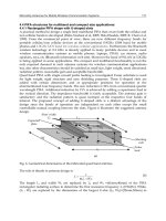
Fig. 9 C-scan image of a bonded structure obtained by high-
frequency acoustic imaging. Center frequency of
the probe was 50 MHz. The color scale (gray scale) is c
alibrated in relative intensity (dB). The width of the

image is 16 mm. Original image is in color. Further details are explained in text.

Scanning Laser Acoustic Microscopy
Principles of SLAM
The operating principle of a SLAM is outlined in Fig. 10. A sample is insonified under a certain angle with respect to the
surface of the sample. In a homogeneous sample, the ultrasound causes a ripple of the surface, off which a laser beam is
reflected. The spatial and temporal periodic displacements of the surface cause the laser beam to be partially diffracted
and frequency to be shifted by the Doppler effect. By a knife edge, one diffraction order is blocked. This then leads to an
alternating current (ac) in the photodiode, because its output contains a mixing product between the undiffracted zero
order and the still-present diffracted part. The frequency of the ac component is equal to the sound frequency, and its
magnitude is proportional to the sound amplitude.

Fig. 10 Schematic showing key components
and parameters of SLAM. The sound waves traveling through the
sample under an angle, , generate a surface ripple with a wavelength of /sin
. The soundwaves are
detected by an optical knife-edge device in which the angle of reflection, , is modulated by an amount,
,
depending on the local amplitude of the surface ripple, according to the amount of scattering by defects present
in the sample. The images obtained are acoustic holograms equivalent to Gabor holography in its original form.
A quadrature receiver is used
to detect the phase of the image required for holographic reconstruction. Here,
the reference phase necessary for quadratic detection is obtained from the rf source driving the transducer. The
images are obtained in real-time (that is, with 25 frames/second).
This technique makes possible the detection of coherent surface waves of extremely small amplitude ( 10
-6
nm/
bandwidth). When pores, inclusions, and cracks are present in the sample, the sound wave is scattered by these defects,
which in turn become visible as a modulation of the otherwise homogeneous surface ripple. By rastering the laser beam
over the surface of the sample, this modulation can be measured and displayed on a television screen (the rate of image

buildup is the TV rate). The resolution in such images is given by the wavelength of the ultrasound and is typically 50 m
in most solid materials at 100 MHz.
It is obvious that the images obtained by SLAM are acoustic shadowgraphs, provided the size of the imaged structure is
large compared with the wavelength. If the size becomes comparable to , diffraction patterns are obtained. If the surface
of the sample is not optically reflective, the dynamic ripple caused by the sound field is then transmitted to a light-
reflecting layer that is coupled acoustically to the sample surface by water.
Reconstruction of Images by Holography
In addition to the simple detection of defects in a given sample, SLAM techniques can be used to study their
characterization and sizing. In general, this is a complex problem, because the SLAM provides two-dimensional images
of a three-dimensional defect geometry deblurred by diffraction effects. Therefore, a defect appear much larger than it
really is. It is possible, however, to detect both the amplitude and phases of the acoustic field in a SLAM image, allowing
reconstruction of the defect by acoustic holography techniques (Ref 23).
Acoustic holography is a two-step process. First, the amplitude and phase of the acoustic field emanating from an
insonified object are detected in a plane adjacent to its surface. Second, from these field data, the scattered field in the
defect plane, , can then be reconstructed with a resolution of 1 wavelength. The relation between the fields (x,y,0)
and (x,y, z) in two parallel planes in the sample under investigation, separated by a distance z, is given by a linear
filtering process (Ref 24):
(k
x
,k
y
,k ) =
0
(k
x
,k
y
,0) · exp (ik
z
· z)

(Eq 4)
where k
z
= and is the corresponding fields in k-space. k
x
and k
y
can be interpreted as the x- and y-
component of the wave vector of a plane wave with amplitude
0
. Thus, the field distributions between the detection
plane and the object can be obtained by calculating the two-dimensional Fourier transform of the field , multiplying it
with the filter function exp(- k
z
· z), and Fourier back-transforming it into spatial coordinates. This process is called
back-propagation. Because outside + = k
2
the filter function is steeply increasing, the filtering is restricted to the
innerface of the circle with radius k so that noise is reduced. The SNR in the back-propagated image can be further
enhanced by deconvoluting the field data with the transfer function of the laser detection scheme employed in the SLAM,
resulting in a total improvement of the SNR of approximately 10 dB compared with the original image.
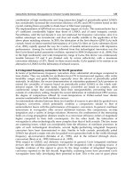
Figure 11 shows the image of an iron inclusion in an Si/SiC bending bar obtained at an ultrasonic frequency of 100 MHz
(Ref 24). The diffraction of the sound-field waves at the inclusion causes concentric ring patterns. Such images are typical
for SLAM. However, by subsequently calculating the field distributions in planes of increasing depth, an image with an
apparently optimal defect contrast is obtained that corresponds to the depth of the defect.

Fig. 11 SLAM image of an iron inclusion in an Si/SiC bending bar as obtained at the output detector. (a) z
= 0

mm (the plane of detection at the surface of the sample). (b) to (f) Reconstructed images at various z
(in
increasing steps of 200 m). As can
be seen in (c) and (d), the defect appears focused, yielding a depth of
approximately 500 m. SLAM parameters: ultrasonic frequency, 100 MHz; field of view, 2.8 × 2.8 mm
2
.
Source: Ref 24

Summary
Acoustical imaging has gained tremendously from the comprehensive theoretical description of the contrast mechanisms
involved and from the availability of high-speed computers. Such computers allow modeling and interpretation of the
complex contrast underlying acoustic images and efficient handling of the large amount of data involved. Applications are
primarily in NDE and materials characterization; some of these applications are related to problems in tribology. In the
future, high priority must be given to the integration of software that permits the reconstruction of defects by synthetic
aperture techniques (Ref 2, 25, 26) and the use of robotic scanning systems in order to scan components of complex
shape.
References
1. C.F. Quate, A. Atalar, and H.K. Wickramasinghe, Acoustical Microscopy With Mechanical Scanning
A
Review, Proc. IEEE, Vol 67, 1979, p 1092-1113
2. A. Briggs, An Introduction to Acoustic Microscopy, Microscopy Handbooks,
Vol 12, Oxford University
Press, 1985
3. P. Höller and W. Arnold, Micro-Non-Destructive Testing of the Structure of New Materials,
Conference
Proceedings of Ultrasonics International 1989, Butterworth Scientific, 1989, p 880-888
4. L.W. Kessler and D.E. Yuhas, Acoustic Microscopy 1979, Proc. IEEE, Vol 67, 1979, p 526-536
5. R. Weglein, Acoustic Micro-Metrology, IEEE Trans. Sonics Ultrasonics, Vol SU-32, 1985, p 225-234
6. A. Atalar, Improvement of the Anisotropy Sensitivity in the Scanning Acoustic Microscope,

IEEE Trans.
Ultrasonics, Ferroelectrics, Frequency Control, Vol 36, 1989, p 164-273
7. J.I. Kushibiki and N. Chubachi, Material Characterization by Line-Focus Beam Acoustic Microscope,
IEEE
Trans. Ultrasonics, Ferroelectrics, Frequency Control, Vol SU-32, 1985, p 189-212
8. R. Weglein, SAW Dispersion in Diamond Films on Silicon by Acoustic Microscopy, Rev. Quant. NDE,

1992 (to be published)
9. A. Atalar, L. Degertekin, and H. Köymen, Acoustic Parameter Mapping
of Layered Materials Using a
Lamb's Wave Lens, Proceedings of 19th International Symposium on Acoustical Imaging,
H. Ermert and
H.P. Harjes, Ed., Plenum Press, 1992 (to be published)
10.

J. Attal, L. Robert, G. Despaux, R. Capalin, and J.M. Saurel, New De
velopments in Scanning Acoustic
Microscopy, Proceedings of 19th International Symposium on Acoustical Imaging,
H. Ermert and H.P.
Harjes, Ed., Plenum Press, 1992 (to be published)
11.

A. Kulik, G. Gremaud, and S. Sathish, Direct Measurements of the SAW Ve
locity and Attenuation Using
Continuous Wave Reflection Scanning Acoustic Microscope (SAMCRUW), Acoust. Imaging,
Vol 18,
1991, p 227-236
12.

K.K. Liang, S.D. Benett, B.T. Khuri-

Yakub, and G.S. Kino, Precise Phase Measurements With the Acoustic
Microscope, IEEE Trans. Sonics Ultrasonics, Vol SU-32, 1985, p 266-273
13.

S.W. Meeks, D. Peter, D. Horne, K. Young, and V. Novotny, Microscopic Imaging of Residual Stress
Using a Scanning Phase-Measuring Acoustic Microscope, Appl. Phys. Lett., Vol 55, 1989, p 1835-1837
14.

H. Vetters, E. Matthaei, A. Schulz, and P. Mayr, Scanning Acoustic Microscope Analysis for Testing Solid
State Materials, Mater. Sci. Eng., Vol A122, 1989, p 9-14
15.

C.H. Chou and B.T. Khuri-Yakub, Acoustic Microscopy of Ceramic Bearing Balls, Acoust. Imaging,
Vol
18, 1991, p 197-203
16.

K. Yamanaka, Y. Enomoto, and Y. Tsuya, Acoustic Microscopy of Ceramic Surfaces, IEEE Trans.
Sonics
Ultrasonics, Vol SU-32, 1985, p 313-319
17.

K. Yamanaka, Study of Fracture and Wear by Using Acoustic Microscopy,
Ultrasonic Spectroscopy and Its
Applications to Materials Science,
Y. Wada, Ed., Special Reports of Japanese Ministry of Science,
Education and Culture, 1988, p 44-49
18.

S. Pangraz, E. Verlemann, and T. Holstein, unpublished results

19.

I. Ishikawa,
T. Semba, H. Kanda, K. Katakura, Y. Tani, and H. Sato, Experimental Observation of Plastic
Deformation Areas, Using an Acoustic Microscope, IEEE Trans.
Ultrasonics, Ferroelectrics, Frequency
Control, Vol 36, 1989, p 274-279
20.

I.N. Ermolov, The Reflection of Ultrasound From Targets of Simple Geometry, Nondestr. Test.,
Vol 5,
1972, p 87-91
21.

S. Pangraz, H. Simon, R. Herzer, and W. Arnold, Non-
Destructive Evaluation of Engineering Ceramics by
High-Frequency Acoustic Techniques, Proceedings of the 18th I
nternational Symposium on Acoustical
Imaging, G. Wade and H. Lee, Plenum Press, 1991, p 189-195
22.

R.S. Gilmore, K.C. Tam, J.D. Young, and D.R. Howard, Acoustic Microscopy from 10 to 100 MHz for
Industrial Applications, Philos. Trans. R. Soc. (London), Vol A320, 1986, p 215-235
23.

Z. Lin, H. Lee, G. Wade, M.G. Oravecz, and L.W. Kessler, Holographic Image Reconstruction in Scanning
Laser Acoustic Microscopy, IEEE Trans. Ultrasonics, Ferroelectrics, Frequency Control,
Vol 34, 1987, p
293-300
24.

A. Morsc
h and W. Arnold, Holographic Reconstruction by Back Propagation of Defect Images Obtained by
Scanning Laser Acoustic Microscopy, Proceedings of 12th World Conference on NDT,
J. Boogard and
G.M. van Dijk, Ed., Elsevier Science, 1989, p 1617-1620
25.

V. Schmitz, W. Müller, and G. Schäfer, Synthetic Aperture Focusing Technique
State of the Art,
Proceedings of 19th International Symposium on Acoustical Imaging,
H. Ermert and H.P. Harjes, Ed.,
Plenum Press, 1992 (to be published)
26.

K.J. Langenberg, Applied Inverse Problems for Acoustic, Electromagnetic and Elastic Scattering,
Basic
Methods of Tomography and Inverse Problems, P.C. Sabatier, Ed., Adam Hilger, Bristol, 1987, p 125-467


Microindentation Hardness Testing
Peter J. Blau, Oak Ridge National Laboratory

Introduction
MICROINDENTATION (MICROHARDNESS) HARDNESS TESTING is an important tool for characterizing the near-
surface characteristics of materials, surface treatments, and coatings. It is extensively used in both applied and research
aspects of tribology. It is a subgroup of the general field of penetration hardness testing, but the relatively low applied
forces (typically, 0.01 to 10 N, or 1 to 1000 gf) make it particularly sensitive to the near-surface mechanical properties of
materials. Some common uses of microhardness testing include:
• Investigating the variations in penetration hardness between various phases in a microstructure

• Initial characterization of the surfaces of materials for wear applications
• Quality control of surface treatments or coatings
• Profiling the depth of hardened surface layers and coatings
• Assessing the nature of subsurface damage on or below machined surfaces
• Assessing the nature of subsurface damage on or below wear surfaces
In addition to hardness number determination, there are other specialized uses of microindentation techniques in friction
and wear technology. These include:
• Use of microindentations as wear markers (see the section
"Wear Measurement Using
Microindentations" in this article)
• Use of microindentations to generate cracks to determine fracture toughness of brittle materials (Ref 1)
The development of instrumented microindentation testing equipment in recent years permits direct monitoring and
recording of the instantaneous force versus the displacement depth for hardness tests. Such equipment offers the
advantage of not requiring optical measurement of the indentation. However, it demands very accurate penetration depth
calibrations. This type of testing is described in the article "Nanoindentation" in this Section. In this article, the focus will
be on more traditional tests involving optical microscopy measurement of the impressions.
Principles of Microindentation Testing
The purpose of microindentation hardness testing is to obtain a numerical value that distinguishes between the relative
ability of materials to resist controlled penetration by a specified type of indenter which is generally much harder than the
material being tested. (A notable exception is in the microindentation testing of very hard materials, like diamond, where
the indenter and test specimen can be equal or nearly equal in hardness.)
After preparing the specimen via the application of good metallographic practice in order to avoid residual damage to the
test surface, the testing procedure involves the following sequence of steps:
1. Mounting the prepared specimen so that its test surface is perpendicular to the direction of indentation
2. Causing the indenter to move downward and impinge on the surface of the specimen at a specified rate
3. Allowing the indenter to remain for a specified residence time after it stops moving
4. Retracting the indenter
5. Measuring a characteristic dimension of the residual indentation
6. Using the geometry of the indenter to calculate a hardness number
Nearly all commercially available microindentation hardness testers perform steps 2 through 4 automatically.

The accuracy and reliability of the numbers obtained in performing microindentation hardness tests are strongly
dependent on three factors: the machine, the operator, and the material characteristics. The machine must be correctly
calibrated for both the applied force and the optical measuring accuracy. It must also be isolated from vibrations during
the test. The operator must be familiar with the correct mounting and specimen preparation methods (such as rigidly
mounting the specimen, keeping the test surface level, and using sound metallographic polishing practice to avoid the
introduction of factors detrimental to specimen preparation), capable of measuring indentations consistently and correctly,
able to recognize invalid indentations, and aware of the need to avoid touching the machine during its operation. The
material may not be homogeneous or the method of fabrication applied in its production may give it hardness numbers
significantly different from those published in tables of "typical values."
One of the greatest sources of error in determining microindentation hardness numbers is in the reading of the indentation
lengths. This problem becomes particularly important when hard materials are being tested or low forces are being used.
Hardness numbers should not be operator dependent. Therefore, all the individuals using the given hardness tester should
be tested to see how closely the measurements of indentation length agree on the same set of reference impressions.
Personal correction factors may need to be given to each person so that measurements on reference specimens agree.
Well-polished austenitic stainless steel or nickel specimens are good for laboratory optical reading reference specimens
because they tend to provide nicely shaped impressions and remain untarnished. Periodic rechecking, approximately once
a year, is desirable because an individual's vision is subject to change. If a critical series of measurements are to be made
more frequently, then recalibration must be performed before each series is started.
If the hardness testing apparatus does not read directly in micrometers, each reader should be familiar with the proper
eyepiece ("filar") unit-to-micrometer conversion method. A "filar" unit is a unit of measure that relates to a scale that is
visible in the measuring eyepiece of the testing machine. If the filar eyepiece is used with different objective lenses, the
conversion between the filar units and micrometers must be obtained for each objective lens. This conversion factor is
derived by measuring the number of filar units that correspond to the observed spacings on a precision, etched microscope
slide that is graduated directly in micrometers ("stage micrometer"). As noted above, each individual using the system
should have his or her own personal filar factors to maintain consistency within the laboratory.
The numerical values obtained by microindentation hardness testing techniques are dependent on a combination of
material properties (for example, elastic modulus, compressive yield strength, mechanical properties, anisotropy, and so
on) that interact under the stress state imposed by the indenter. Therefore, hardness numbers should not be considered
basic properties of a material or a coating, but rather numbers that indicate the response of a given material to the imposed
conditions of the penetration test.

The two most commonly used microindentation techniques are the Vickers and the Knoop microindentation tests. Other
indenter geometries have been developed for special purposes. These will not be discussed here; the reader is instead
referred to books, published standards, and review articles included in Ref 2, 3, 4, 5, 6, 7, 8, 9, and 10.
Most commercial microindentation hardness testers still in use today use gages calibrated in gram-force (gf). However,
the correct International Organization for Standardization (ISO) unit for force (that is, "load") is the Newton (N). Aside
from the hardness scales that report a relative index or number of dimensionless units (such as Rockwell hardness
numbers), indentation hardness numbers are commonly expressed in units of pressure. Units of force and pressure are
related to the traditional microindentation hardness units as follows:

To convert from

To Multiply by

gf
N 0.00981
kgf
N 9.81
kg/mm
2

GPa 0.00981
GPa
kg/mm
2


102.0

Historically, Knoop microindentation hardness is calculated as force per unit of projected area of the indentation, whereas
the Vickers hardness (sometimes known as diamond pyramid hardness, or DPH) is expressed as a force per unit facet

area. This difference in the area is one factor that can lead to slightly different hardness numbers under the same applied
indenter force, especially at relatively low indenter loads (that is, 0.01 to 1 N, or 1 to 100 gf); Knoop numbers are usually
higher than Vickers numbers obtained at the same load.
Standard Reference Materials for Microindentation Hardness
The U.S. National Institute of Standards and Technology, or NIST (formerly the National Bureau of Standards, or NBS),
in Gaithersburg, MD, has developed materials whose microhardnesses can be used for calibration purposes. Known as
Standard Reference Materials (SRM), they can be purchased for either Knoop testing or Vickers testing over the range of
0.25 to 0.98 N (25 to 100 gf). Each specimen comes with a certificate and a set of microhardness numbers for that
specimen. Both materials are electroformed deposits and have the designations listed in Table 1.
Table 1 Standard reference materials used to calibrate Knoop and Vickers microindentation hardness
equipment
Catalog No.

Scale Material

Microhardness,

kg/mm
2

SRM 1893
Knoop Copper 125
SRM 1894
Vickers

Copper 125
SRM 1895
Knoop Nickel 550
SRM 1896
Vickers

Nickel 550

Vickers Microindentation Hardness Test
The Vickers indenter is more widely used throughout the world than the Knoop indenter. The face-to-face angle of the
Vickers indenter was selected so that Vickers hardness numbers would be comparable to those obtained from the
established Brinell hardness test that preceded it. It was recognized that the diameter of Brinell hardness indentations (d
B
)
varied between 0.25 and 0.5 times the ball diameter (D
B
). Using the mean of d
B
= 0.375 D
B
gave a ratio of surface contact
area to the projected area (circular area of the indentation viewed from above) for the Brinell case of 1.08:1. This ratio is
approximately the same for a Vickers pyramid when the face-to-face apex angle is 136°; hence, this angle was chosen for
the Vickers pyramid. Figure 1 shows the shape of the tip of a Vickers hardness (diamond pyramid hardness) indenter and
defines the symbols used in subsequent equations.

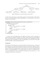
Fig. 1 Key dimensions and geometry for the tip of a Vickers indenter. (a) Diagonals d and d . (b) Face-to-
face apex angle
There is some confusion in the literature as to the symbols used for microindentation hardness numbers using the Vickers
indenter. Three commonly used symbols are DPH, VHN, and HV
P
, where P represents the applied force. The later
symbol is preferred by ASTM.
The general equation for Vickers hardness uses the average value of the two diagonals, d*, where

(Eq 1)
to calculate the hardness value


(Eq 2)
where P is the applied force, usually expressed in units of grams-force or kilograms-force, and C
V
is a proportionality
constant.
Vickers Indenter Versus Knoop Indenter. The Knoop indenter has both advantages and disadvantages over the
Vickers indenter in microindentation testing. Because it is more blunt, the Knoop indenter tends to promote less cracking
during the indentation of brittle materials (the penetration depth is 0.635 that of the Vickers indenter, assuming equal test
force and hardness number). Impressions are long and narrow, allowing the Knoop indenter to be used for hardness
testing of thin layers or of narrow microstructural constituents. With the lower symmetry of the Knoop impression
compared to the Vickers impressions, it tends to be somewhat more sensitive to crystallographic anisotropy than the
Vickers indenter. The general shape of the ideal Knoop indenter tip and the symbols used in this section are shown in Fig.
2.

Fig. 2 Facets, dimensions, and geometry of a Knoop indenter tip. (a) Three-di
mensional view of tip of Knoop
indenter. (b) Diagonals D and d, where ratio of D/d is 7.1143. (c) Major (172.5°) and minor (130°) apex angles

Rather than requiring the averaging of two indentation diagonals, as in the case of the Vickers hardness calculation, the
Knoop method requires only that the length of the longer diagonal, D, be measured. With the advantage of only one
measurement per indentation comes the tendency for increased susceptibility to anisotropy in surface mechanical
properties. The Knoop microindentation equation is


(Eq 3)

Table 2 gives the values for the proportionality constants C
V
and C
K
for various choices of units.

Table 2 Proportionality constants for Vickers and Knoop hardness scales as a function of hardness, force,

and diagonal length
Constant Applicable property value
C
K

C
V
Hardness

Force, P

Diagonal length

Knoop (HK)
1.423 × 10
4


. . . kg/mm
2
gf
D, m

1.423 × 10
7


. . . kg/mm
2
kgf
D, m
1.396 × 10
2


. . . GPa gf
D, m
1.396 × 10
5


. . . GPa kgf
D, m
Vickers (HV)
. . .
1.854 × 10
3


kg/mm
2
gf
d*, m

. . .
1.854 × 10
6


kg/mm
2
kgf
d*, m
. . .
1.819 × 10
1


GPa gf
d*, m
. . .
1.819 × 10
4


GPa kgf
d*, m

Microindentation Hardness Numbers of Materials
In the previous discussion, it was stated that microindentation hardness of materials depends not only on the composition
of the material but also on the quality of the surface preparation, the method by which the material was produced, the
indenter used, and the normal force (load) on the indenter. Therefore, the microindentation hardness numbers provided in
this article are to be used only as a general guide to typical values for various materials. Owing to differences in surface
preparation and microstructural condition, it is always better to obtain values on the specific specimen of interest than to

use table values. Table 3 lists Vickers and Knoop microindentation hardness numbers that have been obtained on selected
materials.
Table 3 Vickers and Knoop microindentation hardness numbers for selected materials

Hardness numbers Material Form
(a)
Force, gf

HV, GPa

HK, GPa

Ref

Pure metals
polyxl., 99.99% 10 0.25 . . . 11
Aluminum
<100> on [100] xl. plane 50 0.227 12
25 0.21 0.21 13
50 0.19 0.22 13
Cadmium
High purity, polyxl.
100 0.19 0.23 13
Carbon
Diamond 200 98.65 . . . 14
25 2.46 2.88 13
50 2.71 3.34 13
Cobalt
High purity, polyxl.
100 2.59 2.73 13

25 0.57 0.48 13
50 0.46 0.41 13
Copper
High purity, polyxl.
100 0.42 0.37 13
Polyxl. 20 0.66 . . . 11
Gold
. . . 10 . . . 0.77 15
25 2.44 2.92 13
50 2.49 2.92 13
Iron
High purity, polyxl.
100 2.44 2.76 13
Lead
Creeps at room temperature

5 0.049 . . . 1
Magnesium
Cast, 99.8-9% pure 40 0.47 . . . 11
25 2.90 3.32 13
50 2.73 2.76 13
Molybdenum
High purity, polyxl.
100 2.73 2.76 13
25 1.00 1.06 13
50 1.03 1.04 13
Nickel
High purity, polyxl.
100 1.01 1.14 13
. . . 10 14.22 . . . 15

Phase in aluminum alloy 50 . . . 8.83 15
Silicon
Phase in aluminum alloy 100 . . . 13.7 13
Silver
Coinage grade 20 0.94 . . . 11
Titanium
Annealed 60 1.54 . . . 11
Single crystal (0001) 10 0.163 . . . 11
Zinc
Single crystal (1450) 10 0.323 . . . 11
Bearing steel
50 8.41 . . . 13
AISI 52100
Ball
100 8.41 9.80 13
Carbides and nitrides
Boron carbide
BC 50 23.54 . . . 15
Chromium carbide

Cr
3
C
2
. . . 19.12 . . . 15
Hafnium carbide
. . . 50 28.57 . . . 15
. . . 25 17.65 . . . 15
(Green) 100 24.53 15
Silicon carbide

Another source (gray) 100 38.25 15
. . . 31.38 . . . 11
Titanium carbide
. . .
100 24.23 . . . 15
WC . . . 15.69 . . . 11
WC 100 16.30 18.44 15
Tungsten carbide
WC
2
50 29.42 . . . 15
30 . . . 21.18 15
Titanium nitride
TiN
100 . . . 17.36 15
Oxides
-Al
2
O
3

100 24.5 . . . 11
Aluminum oxide
Sapphire 100 25.5 . . . 11
Magnesium oxide
MgO, single xl. 50 11.2 . . . 11
Silicon dioxide
SiO
2
. . . 11.8 . . . 11

Titanium dioxide
Rutile 25 9.8 . . . 11
Yttriuim oxide
Y
2
O
3
. . . 6.86 . . . 11
Source: Ref 11, 12, 13, 14, 15
(a)
xl., crystalline; polyxl., polycrystalline.

Microindentation Testing of Coatings
Film-covered surfaces and coated surfaces present special problems for micromechanical properties and hardness
determination, especially if the properties of the thin layer(s) are to be separated from those of the substrate. Sometimes it
is not necessary to separate the properties of the surface layer from those of the substrate if it is the materials system and
not its constituent parts that is functionally important in the given application.
Single-Layer Coated Surfaces. Figure 3 indicates two of the four possible situations that can occur when indenting a
surface covered by a film or a coating. In Fig. 3(a), the indenter moves directly through the coating layer without
disturbing the coating of thickness t. In actual physical situations, it is unlikely that this situation will occur. The coating
that originally occupied the volume now taken up by the indenter tip must go somewhere. If it behaves in a ductile
manner, some of the coating material will be displaced to the side of the indenter and other portions may be drawn down
into the indentation (Fig. 3b). Some materials that are normally considered to be brittle may behave in a ductile manner
under the highly localized and confined compressive stresses beneath a sharp indenter tip.

Fig. 3
Schematics showing two possible reactions of a coating layer to indentation. (a) In the ideal case,
indenter moves directly through coating layer without disturbing coating thickness. (b) If coating reacts in a
ductile manner, the coating is drawn into the depression generated by the downward motion of the indenter tip.

The third possible reaction can occur if the coating contains significant levels of residual stress, if it adheres poorly to the
substrate, if it is precracked, or if it is extremely brittle. That is, the coating will fracture or spall off in the neighborhood
of the indentation. Trying to make sense of the hardness numbers obtained in this catastrophic coating failure is not
worthwhile. In the fourth case, the coating may conform to the shape of the indenter and be pressed into the substrate
without any change in thickness or the onset of fracture.
For the case where a portion of the coating material is drawn inward and another portion piles up to the side, the
minimum facet contact area, f, occupied by the coating of thickness, t, when penetrated to a depth, z
1
, can be determined
by the equation:


(Eq 4)
From Eq 4, even when the penetration depth is twice the coating thickness, at least 75% of the indenter facet area is
occupied by coating material. If the coating material is drawn into the indentation, this percentage may be higher, but the
thin layer of coating material that coats the substrate at the bottom of the indentation is unlikely to have as important an
effect on the load-bearing as the substrate itself.
Another issue involved with layered or coated surfaces is the strength of the bonding between the coating and the
substrate. The action of indenting the surface may cause coating delamination to occur as the surrounding material
buckles up and comes away from the substrate. Using this phenomenon, spherical indenters have been used in tests of
polymer film bonding (Ref 16).
Several treatments for coating hardness have involved a rule of mixtures for the effective hardness number, H
comp
. In one
such treatment developed by P.J. Burnett and D.S. Rickerby (Ref 17), H
comp
is determined to be:
H
comp
= f

c
H
c
+ f
s
H
s
X
3


(Eq 5)
where f
c
and f
s
are the respective volume fractions of coating and substrate materials being deformed; H
c
and H
s
are the
respective coating and substrate hardnesses; and X is the interfacial parameter. The constraint parameters were found to
be strongly dependent on the relative radii of the substrate and coating plastic zones. Also, for a weakly bonded film, the
constraint parameter was closer to 1.0.
Jonsson and Hogmark (Ref 18) have developed an alternate formulation with the hardness of the film, H
f
, given as:


(Eq 6)

where H
s
and H
c
are the hardnesses of the substrate and the composite, respectively; D is the penetration depth (for
Vickers, diagonal length/7); t is the film thickness; and C is the constant whose value depends on whether the film is
brittle or whether it deforms to match the indenter shape. In the brittle case C is 0.0728, and in the ductile case C is
0.1403.
The use of two different treatments for the ductile and for the brittle films leads to the important issue of hard film on
softer substrate versus soft film on harder substrate. The latter case is sometimes associated with the so-called "anvil
effect." To obtain a "valid" hardness number for a material, ASTM standard E 384 requires that the penetration of the
specimen material must be no more than one-tenth its thickness. This is a conservative position, because in some specific
cases, the zone of affected material may extend to less than five times the thickness. In the absence of additional
information about the material of interest, a factor of ten is generally reliable. If the penetration is not through the film or
the coating, but represents say, one-half of its thickness, one would expect to see some effect on the hardness number by
the substrate. Conversely, if the penetration depth is many times the film thickness, the effect of the film is expected to be
negligible. In one case where a submicron film of electrodeposited chromium on copper was Vickers hardness tested, it
was found that the effect of the film was no longer significant when the penetration depth exceeded about twelve times
the coating thickness.
When testing thin films or coatings, it is advisable to use a series of indentation loads. In doing so, a range of effects in
the coating/substrate system can be examined. Empirical formulations can then be derived for comparing one coating
system with another.
Multilayer coating systems (for example, electrical contacts) are even more complex to analyze mechanistically. The
interaction of more than two constituents with different mechanical properties and the interfacial constraints between
layers need to be considered. Scratch tests of various types are often used to assess the adhesion and durability properties
of coatings. Scratch testing is a separate subject that is discussed in the article "Scratch Testing" in this Section.
References 19, 20, 21, 22, 23, 24, 25, and 26 may be helpful in regard to the microindentation testing of thin films and
coatings. Some of these references use the nanoindentation techniques described elsewhere in this Volume.
Wear Measurement Using Microindentations
By utilizing the geometrical properties of microindentations, it is possible to estimate the amount of surface recession due

to wear. For example, the ratio of the indentation depth to the length of the major diagonal of a Knoop indentation is
1:30.5, and the ratio of the depth of a Vickers indentation to the length of a diagonal is 1:7.00. These techniques can be
applied only under the following two conditions:
•
Wear surface material exhibits only a minor amount of elastic recovery after indentation, or the amount
of elastic shape recovery is known
•
Wear taking place is mild enough that the edges of the impressions are not unduly distorted or covered
over
Microindentations can be used to measure mild wear in several ways:
• Method 1: periodical plastic replication of microindentations p
laced on the inside of a bushing or other
normally inaccessible wear surface
• Method 2:
calculation of incremental wear rate by measuring the changes in the dimensions of
indentation diagonals
• Method 3: the smallest remaining indentation in a series that
was originally produced at a succession of
increasing loads
Method 1 (Ref 27). W.A. Glaeser used a Knoop indenter on the tip of a rigid rod tap a reference indentation inside a
bronze bushing. By periodic replication of the indentation using plastic, Glaeser was able to watch the progression of
wear in the bushing. In such cases, it would be advisable to place impressions at several locations because wear may vary
from place to place on the contact surface of the bushing.
Method 2 makes use of the geometrical properties of indentations. When using this method, one assumes that the
indentation geometry is similar to the indenter that produced the indentation. If substantial elastic shape recovery of the
indentation occurs following the withdrawal of the indenter, then this method can only be considered to be approximate.
By using the relationships between depth and diagonal length for Vickers and Knoop indenters, one can estimate a change
in depth due to a change in the diagonal length due to wear:

(Eq 7)
where z is the incremental wear depth, d
0
is the length of the diagonal of the hardness indentation before wear occurs, d
f
is
the length of the indentation diagonal after wear occurs, and C is a constant whose value is dependent on the type of
indenter used to generate the indentation. For a Vickers indentation with no significant elastic recovery in the surface, the
value of C is 7.00; for a Knoop indentation with no significant elastic recovery in the surface, the value of C is 30.52.
This technique may be useful for measuring very small amounts of wear (for example, polishing). However, it is not
effective when the wear process obscures the ends of the indentations. This method has been applied to determine wear
patterns on magnetic recording heads (Ref 28).
Method 3 involves placing one or more rows of Knoop or Vickers indentations, produced at a series of loads, on the
preworn surface of the specimen. After wear, the observer should note the smallest remaining indentation. Because a
certain depth can be associated with each indentation, removal of a complete indentation indicates an increment of wear.
If the hardness versus applied force behavior of the surface is known, indenter forces can be selected to give relatively
equal depth increments. This wear measurement method has been suggested by L.K. Ives of the National Institute of
Standards and Technology.
Correlation of Microindentation Hardness Numbers with Wear
There are many kinds of wear, as indicated in the Section titled "Wear" in this Volume. The types of localized stresses
and directions of relative motion vary considerably between the various kinds of wear. Sometimes the stress conditions
experienced by a wear surface are more similar to those imposed during a microindentation hardness test than in other
cases. This means that the correlation between numerical values of microindentation hardness and wear rates may not
necessarily correlate. Classic Russian studies of abrasive wear have established relationships of relative hardness to
relative wear rates (Ref 29). However, this relationship does not always hold. There may not necessarily be a correlation
between microindentation hardness numbers of the unworn surface and wear due to the following reasons:
Workhardening. In wear of metals and alloys, contact surfaces may change hardness greatly due to work hardening
during wear. Therefore, using initial hardness numbers may be misleading.
Differences in Stress State. In a traditional hardness test, the indenter moves vertically down and up. In many forms
of wear, material is deformed tangentially to the plane of the surface giving rise to shear stresses that do not occur in

vertical penetration experiments.
Strain Rate Effects. In hardness testing, the rate of indentation (strain rate) may be small compared to that experienced
by the same surface during wear. At high strain rates, materials are known to change their mechanical properties, often
increasing in stiffness and yield strength.
Thermal and Chemical Contributions to Wear. Microindentation hardness numbers obtained under normal room
environments may not accurately portray the mechanical behavior of a wear surface that is heated by friction.
Furthermore, tribochemical effects such as oxidation or film formation may dominate wear behavior in ways that cannot
be described by hardness numbers.
Third Bodies and Films. The microindentation hardnesses of the original surfaces may not bear any relationship to the
properties of the material that accumulates on the wear surface during prolonged contact and that eventually governs wear
behavior.
Effects of Brittleness. While many materials wear better if their surfaces are hardened, it is also true that very hard
materials may be brittle and thus subject to fracture under the action of wear. The relationship of microindentation
hardness to wear resistance may not be established for very brittle materials because the data simply cannot be obtained.
References
1. G.R. Anstis, P. Chantikul, B.R. Lawn, and D.B. Marshall, J. Am. Ceram. Soc., Vol 64 (No. 9), 1981, p 533
2. D. Tabor, The Hardness of Metals, Clarendon Press, Oxford, 1951
3. B.W. Mott, Microindentation Hardness Testing, Butterworths, London, 1957
4. H. Bückle, Progress in Micro-Indentation Hardness Testing, Met. Rev., Vol 4, 1959, p 49-100
5. D.R. Tate, A Comparison of Microhardness Indentation tests, ASM Trans., Vol 35, 1945, p 374-389
6. J.H. Westbrook and H. Conrad, Ed., The Science of Hardness Testing and Its Research Applications,

American Society for Metals, 1973
7. P.J. Blau and B.R. Lawn, Ed., Microindentation Techniques in Materials Science and Engineering,
STP
889, ASTM, 1985
8. V.E. Lysaught, Indentation Hardness Testing, Reinhold, 1949
9. "Test for Microhardness of Materials," E 384, Annual Book of ASTM Standards, ASTM
10.

"Test for Microhardness of Electroplated Coatings," B 578, Annual Book of ASTM Standards, ASTM
11.

A.A. Ivan'ko, Handbook of Hardness Data,
U.S. Department of Commerce, National Technical Information
Service, 1971, transl. from Russian
12.

B.C. Wonsiewicz and G.Y. Chin, A Theory of Knoop Hardness Anisotropy,
The Science of Hardness
Testing and Its Research Applications, American Society for Metals, 1973
13.

P.J. Blau, compiled from studies done at the National Bureau of Standards, 1980-1983
14.

M.M. Khruschov and E.S. Berkovich, Ind. Diamond Rev., Vol 11, 1951, p 42
15.

B.W. Mott, Micro-indentation Hardness Testing,
Appendix I, Butterworths Scientific Publishing, London,
1956
16.

P.A. Engel and M.D. Derwin, Microindentation Methods in Materials Science and Engineering,
STP 889,
ASTM, 1985, p 272-285
17.

P.J. Burnett and D.S. Rickerby, Thin Solid Films, Vol 154, 1987, p 403-416

18.

B. Jönsson and S. Högmark, Thin Solid Films, Vol 114, 1984, p 257-269
19.

M. Antler and M.H. Drozd
owicz, Wear of Gold Electrodeposits: Effect of Substrate and of Nickel
Underplate, Bell Syst. Tech. J., Vol 58 (No. 2), 1979, p 323-349
20.

E.H. Enberg, Testing Plating Hardness and Thickness Using a Microhardness Tester, Met. Finish.,
Vol 66,
1968, p 48
21.

M. Yanagisawa and Y. Motomura, An Ultramicro Indentation Hardness Tester and Its Application to Thin
Films, Lubr. Eng., Vol 43 (No. 1), 1987, p 52-56
22.

P.I. Wierenga and A.J.J. Franken, Ultramicroindentation Apparatus for the Mechanical Characteriz
ation of
Thin Films, J. Appl. Phys., Vol 55 (No. 12), 1984, p 4244-4248
23.

M. Nishibori and K. Kinosita, A Vickers Type Ultra-Microhardness Tester for Thin Films,
Jpn. J. Appl.
Phys., Vol 11, 1972, p 758
24.

J.B. Pethica, R. Hutchings, and W.C. Oliver,

Composition and Hardness Profiles in Ion Implanted Metals,
Nucl. Instrum. Methods, Vol 209/210, 1983, p 995-1000
25.

M. El-
Shabasy, B. Szikora, G. Peto, J. Szabo, and K.L. Mettal, Investigation of Multilayer Systems by the
Scratch Method, Thin Solid Films, Vol 109, 1983, p 127-136
26.

V.C. George, A.K. Dua, and R.P. Agarwala, Microhardness Measurements on Boron Coatings,
Thin Solid
Films, Vol 152, 1987, p L131-L133
27.

W.A. Glaeser, Wear, Vol 40, 1976, p 135-137
28.

A. Begellinger and A.W.J. de Gee, Wear, Vol 43, 1977, p 259-261
29.

M.M. Khruschov, Proceedings of Conference on Lubrication and Wear,
Institute of Mechanical Engineers,
1957, p 655

Nanoindentation
H. M. Pollock, School of Physics and Materials, Lancaster University (England)

Introduction
ONE REASON for the need to devote a separate article to nanoindentation, as distinct from microindentation, is that the
type of instrumentation and data processing needed for nanoindentation has evolved in a different way. Additionally,

some interesting phenomena that are especially important at the submicron scale occur, such as time-dependent behavior
and the effect of ion irradiation. This article describes how nanoindentation data are obtained and interpreted, and
provides examples of measurements involving polishing wear and other surface effects, surface treatments and coatings,
fine particles, and other technologically important topics.
Nanoindentation Defined. Indentation testing becomes nanoindentation when the size of the indent is too small to be
accurately resolved by optical microscopy. The concern is not solely with hardness and elasticity, because this definitely
can be widened to include other types of tests, such as creep and even friction or film-stress measurement, which can
conveniently be carried out with a nanoindentation instrument. In practice, the term nanoindentation usually implies the
continuous recording of the distance moved by the indenter (penetration depth) and of the load, as well as other variables
(such as time or frictional force), rather than single-valued measurements of contact area, as is usual with
microindentation testing. This is simply because continuous depth recording (CDR) has proved to be the most direct
solution to the problem of measuring very small indent sizes. However, as summarized in Table 1, not all nanoindentation
testing involves CDR, which has its disadvantages. Conversely, CDR has proved to be a valuable addition to conventional
microindentation instruments (Ref 1).
Table 1 Correlation (in practice) between CDR and micro/nanoindentation
Technique Microindentation Nanoindentation
Imaging of indents by
microscopy
Usual One type of commercial instrument only
(Ref 2)
Continuous depth recording
Occasional examples in the scientific literature (see
Ref 3)
Usual

The advantages of CDR include a high level of precision, ease of digitization, automation, and data processing. It is ideal
for the measurement of creep, as well as of plastic and elastic work. Furthermore, each test normally gives a complete
loading/unloading cycle, rather than just a single reading.
As a sole method of measuring indent size, its disadvantage is the need for simplifying assumptions in order to:
• Separate plastic from elastic effects

• Determine the true zero of the depth measurements
• Allow for piling-up or sinking-in of material around the incident
• Allow for geometric imperfection of the indenter when deriving absolute hardness values
Type of Information Obtained. Nanoindentation testing by CDR does not give values of absolute hardness directly.
This is because hardness is usually defined as load divided by indent area projected onto the plane of the surface, and this
area is not explicitly measured. However, the data can be processed on the basis of well-established assumptions (Ref 4)
to yield relatively direct information that is of value in quality control.
This direct information on elastic recovery, relative hardness, work of indentation, and strain rate/stress relationship (Fig.
1) can provide a comprehensive "fingerprint" of a particular sample resulting, for example, from a change in either a
production process or a wear test procedure. It is ideally suited to the comparison of one sample with a control or
reference. The wider assumptions that are needed to derive indirect information on the material properties that are of
particular scientific value are also defined in Fig. 1.

Fig. 1 Types of information obtained
The topic has produced some surprises, as mentioned in an earlier review (Ref 3) that discussed near-surface creep at low
homologous temperatures, and some work in Japan that sometimes found a "critical load," below which no detectable
plastic deformation remains. A number of years passed before independent confirmation was obtained, either
experimentally (Ref 5, 6) or theoretically (Ref 7, 8).
The area under the depth-load curve is related to the work done by the indenter on the specimen. By subtracting the area
under the unloading curve from the total area, W
T
, the work, W
p
, that is retained by the specimen (Fig. 5) is measured. For
an elastic material, all the work is released upon unloading, that is, W
p
= 0 and
p
= 0. For a plastic material, all the work
is retained by the specimen, that is, W

p
= W
T
and
p
=
T
. If the departure from linearity of the unloading curve is
neglected, then:


(Eq 9a)
and because R is defined as '
e
/
p
, with
p
=
T
- '
e
, Eq 2 in the preceding article follows directly. Alternatively, P
m
d
/dP can be substituted for '
e
(Fig. 5), giving Eq 3.
To express R in terms of H and E, it is seen, from Eq 1, that '
e

= (1 - v
2
)P/(2Ea), and that from the definition of k
1
,
p
=
a( /k
1
)
1/2
. Thus, R = '
e
/
p
= P/(2Ea
2
)(k
1
/ )
1/2
. But, from the definition of hardness, P/( H) can be substituted for a
2
, so
that Eq 4 follows.
The quantity H(1 - v
2
)
2
/E

2
, which is independent of k
1
, can be calculated as follows: From Eq 4, H(1 - v
2
)
2
/E
2
= 4R
2
/(
k
1
H), and from the definition of k
1
and I
p
, k
1
H = I
p
, so that Eq 7 follows.
Acknowledgements
The way in which the nanoindentation test procedures are presented in this article reflects many discussions and much
helpful criticism from Dr. R.H. Ion. I am grateful also to Dr. R.C. Rowe, Dr. J. Skinner, Dr. J C. Pivin, and Dr. M.
Ghadiri for providing specimens for Fig. 3, 8, 10 and 12, and 15, respectively.
Nanoindentation Instruments
Where the prime requirement is to obtain absolute values of hardness in the sense of resistance to plastic deformation, a
logical approach is to replace the optical microscope of a microindenter by an electron microscope. A nanoindentation

attachment that can be used inside a scanning electron microscope (SEM), has formed the basis of patents and is
commercially available (Ref 2). In principle, this approach makes it possible to establish a reliable comparison between
nanoindentation hardness values and established scales of hardness numbers, such as those defined in national standards
specifications. It is necessary to overcome the difficulties of imaging small indentations with sufficient contrast, and, at
the smallest depths, to correct for the deformation of the required conductive layer of soft metal (Ref 9). In practice, many
investigators have found the advantages of continuous depth recording to be overriding. Therefore, the discussion that
follows deals primarily with nanoindentation testing using CDR.
The main features of existing instruments are listed in Table 2. Except when adhesion is being measured, the indenter is
virtually always pyramidal, rather than hemispherical, given that the interest is in deformation at very small depths below
the specimen surface. Vickers or Knoop indenters are sometimes used (Ref 1, 10), but a three-sided pyramid is more
common, because this shape can achieve a better approximation to a perfectly pointed apex, either by polishing or by ion
erosion. The apical angles can be chosen so that the nominal relation between indent area and depth is the same as for the
Vickers shape.
Table 2 Potential design features of comprehensive nanoindentation instrument
Basic requirements
Vibration isolation and draft exclusion Indenter: normally a trigonal diamond pyramid
Soft testing designs
Loading device, such as coil in magnetic field
Depth-sensing transducer, such as capacitative, inductive, or fiber-optical
Analog or digital loading control (ramp mode; step mode)
Hard testing designs
Load cell (force-to-voltage transducer)
Displacement actuator
Analog or digital displacement control (ramp mode; step mode)
Data logging system
Data processing software
Options
Environmental enclosure
Optical microscope
Digital x-y-z sample displacement (from one indent position to the next; also, to microscopy location)

Additional ultrasmooth actuator for recalibration of depth transducer
Servocontrol of selected force or displacement
Modulation (ac component) of the load, for compliance measurements
Automatic detection of indenter-specimen contact
Additional programming: approach speed, loading/unloading cycle, series of indents
Vibration detector (data affected by vibration exceeding a set level to be discarded)
Temperature compensation
Hot stage
Friction measurement (smooth lateral displacement; transverse force transducer)
Scratch testing
Profilometry and depth sensing for measurement of film stress, Young's modulus, and other properties


Alternatively, a more acute angle (such as 90° between edges) can be chosen, on the grounds that thinner coatings can be
tested without the data being significantly affected by the properties of the substrate. Also, sharp indenters give more
consistent results when the specimen surface is rough (Ref 11). Like other mechanical instruments, nanoindentation
devices can be either "soft" testing machines, where load is imposed and the displacement measured, or "hard" machines,
where the displacement of the indenter into the specimen is imposed.
With soft machines (Ref 3, 12, 13, 14, 15), indenter and loading device must be mounted on a frictionless suspension.
This often involves elastic design (spring hinges and leaf springs). In one instrument (Ref 13), an air bearing is used
instead, and there is no need for the weight of the indenter to be counterbalanced. To minimize kinetic and impact effects,
the moment of inertia of the moving assembly should be as small as possible. The relative movement of indenter and
specimen (indentation depth) is measured by means of a displacement transducer, which can be a capacitance gage, a
variable mutual inductance, or a fiber-optic device. The specifications of one commercial instrument (Fig. 2) are listed in
Table 3.
Table 3 Commercial nanoindentation instrument specifications
Ultramicrohardness measurement
Typical depth
resolution
<1 nm

X resolution/travel
0.02 m/50 mm
Y resolution/travel
0.02 m/50 mm
Z resolution/travel
0.02 m/25 mm
Repositioning precision
0.1 m
Typical force resolution
20 N
Maximum load
0.5 N (0.11 lbf)
Software
Preprogrammed control and data analysis package with menu-driven facilities for custom program
development
Dimensions
500 × 400 × 300 mm
Stress measurement
Maximum sample size
200 mm diameter
Analysis field
50 × 50 mm square
Data obtained
Film thickness, film and substrate elastic modulus, substrate shape, and film stress
Curvature resolution
( R) corresponds to R > 3 × 10
4
m
Friction measurement
Maximum force

200 mN
Scan length
To 50 mm
Data obtained
Coefficient of static or dynamic friction


Fig. 2 Nanoindentation instrument with CDR; xyz, three-dimensional specimen micromanipulator; H,

removable specimen holder; S, specimen; D, diamond indenter; W, balance weight for indenter assembly; E,

electromagnet (load application); C, capacitor (depth transducer). Courtesy of Micro Materials Limited
With hard machines (Ref 10, 16, 17), the indentation depth is controlled, for example, by means of a piezoelectric
actuator. Force transducers used in existing designs include: a load cell with a range from a few tens of N to 2 N (Ref
17, 18); a digital electrobalance with a resolution of 0.1 N, and a maximum of 0.3 N (Ref 16); and a linear spring whose
extension is measured by polarization interferometry (Ref 10).
As noted in Table 2, it should be possible to vary the load or, in hard machines, the displacement, either in ramp mode or
with a discontinuous increment (step mode). The important effects of varying the ramp speed, that is, the loading rate,
will be discussed in the section "Choosing to Measure Deformation or Flow" in this article. The ramp function needs to be
smooth, as well as linear, and there is evidence (Ref 19) that if the ramp is digitally controlled, the data will vary for the
same mean loading rate according to the size of the digitally produced load increments, unless these are very small.
The basic requirements include a system for data logging and processing. Scatter in nanoindentation data tends to be
greater than with microindentation, partly as a result of unavoidable surface roughness, but principally because the
specimen volume being sampled in a single indentation is often small, compared with inhomogeneities in the specimen
(such as grain size or mean separation between inclusions). Thus, unless such indent is to be located at a particular site, it
is usually necessary to make perhaps five, ten, or more tests, and to average the data.
The spacing between indents must be large enough for each set of data to be unaffected by deformation resulting from
nearby indents, and the total span should be at least one or two orders of magnitude greater than the size of the specimen
inhomogeneities whose effect is to be minimized by averaging. On the other hand, if the test results turn out to be grouped
in such a way that reveals differences between phases or grains, then each group should be averaged separately. In either

case, the number of data points to be processed is large.
A real-time display helps the operator to monitor the data for consistency between indents and for any systematic trend
and arises, for example, from a change in the effective geometry of the indenter, if traces of material from the specimen
become transferred to it. The most common reason for an inconsistent set of data is a vibration transient, the effect of
which is visible at the time. A subjective decision can then be made to discard that particular data set. Rather than use a
real-time display for this purpose, a more reliable approach is to use the output signal from a stylus vibration monitor (a
simple modification of the detection system itself) to abort any individual test during which the vibration exceeds a
certain level.
Options that can greatly increase the scope and convenience of a nanoindentation instrument are listed in Table 2, in
addition to basic requirements. With many specimen types, it is essential to record the exact location of each indent. This
is achieved with the help of a specimen stage driven by either stepping motors or dc motors fitted with encoders.
However, such devices must not be allowed to increase the total elastic compliance of the instrument to a value
comparable with the smallest specimen compliance likely to be measured (the measurement of compliance is discussed in
the section "Slow-Loading Test" of this article).
It is useful to be able to displace the specimen, as smoothly as possible, toward and away from the indenter, as well as to
minimize impact effects at contact. This also facilitates recalibration of the displacement transducer, which in some
designs varies according to the location of the plane of the specimen surface. In at least one design (Ref 3), the specimen
displacement stage allows the surface to be brought into the field of view of an optical microscope, by using computer
control. Another system (Ref 18) uses a closed-loop TV camera to help reposition the indenter rapidly and safely.
Refinements to the electronic hardware and software have been introduced to give, for instance, servocontrol of the
selected load, loading rate, or displacement. This allows automatic compensation for nonideal transducer parameters, such
as finite load cell compliance. Furthermore, the choice of loading mode (constant ramp speed or discontinuous step) can
be extended to include more elaborate modes, such as constant strain rate or constant stress. Useful refinements include
automatic control of the speed with which the specimen approaches the indenter and detection of the instant of contact.
Thus, the whole loading-unloading cycle, and any required series of cycles, can be automated. As described in the section
"Averaging of Multiple Tests" of this article, one design (Ref 6) includes provision for ac modulation of the load, which
allows the continuous measurement of the compliance of the contact.
Of course, drift can be a problem, and attention must be paid to temperature stability. On occasion, temperature
compensation is necessary in connection with depth or load transducers. Thus far, the introduction of specimen heating
stages has been delayed by the consequent major problems of thermal drift.

Other physical measurements that require the use of the transducers mentioned also can be carried out, in principle,
by means of a modified indentation procedure. One example is the determination of Young's modulus for thin films and
other small specimens in the form of simple or composite beams whose elastic compliance is measured (Ref 16). As with
optical scanning techniques, values of film stress can be derived from measurements of deflection and curvature of the
film/substrate composite. Likewise, biaxial tensile testing of free-standing films can be carried out by means of the bulge
test: if the bulge shape is profiled at a number of locations by probing with the indenter, then the strains can be calculated
without the need to assume that the bulge is spherical. In effect, this represents a specialized type of profilometry, of
which other examples include the measurement of film thickness and scratch width, as discussed below.
Film adhesion can be characterized by various methods, two of which can be used, in principle, with the help of a
nanoindentation instrument modified to act as a film failure mechanism simulator. The indentation fracture technique
(Ref 20, 21) has the advantage that normal loading only is required, thus avoiding complications of interpretation that
arise from groove formation. In addition, values of fundamental parameters, such as critical stress-intensity factor, can be
derived, in principle. A variant of the CDR technique, which monitors the load-depth curve, together with acoustic
emission, in order to detect debonding at fiber-matrix interfaces in composites is described in Ref 22.
The thin-film scratch test has successfully been carried out by Wu et al. (Ref 23), who used conical indenters with
hemispherical tips of radii down to l m, and a tangential load cell. These were fitted to a nanoindentation instrument, for
which the servo system could be set to give either constant indentation speed or constant rate of normal loading while the
specimen was being translated at constant speed. As with conventional scratch testing, the critical load at which film
cracking or delamination begins is used as an empirical measurement of adhesion. It was found that a reliable indication
of this load was the value at which a load drop first occurred during a scratch loading curve. Thus, in many cases,
fractography by SEM was not required for the detection of delamination.
Other established methods of detection, such as acoustic (Ref 24) or use of friction signal (Ref 25), can readily be used in
conjunction with this technique. Wu et al. (Ref 18, 23) discuss the prospects of thus deriving values of fracture toughness
of film/substrate assemblies. They also describe how scratch hardness is derived from measurement of the width of the
scratch track when this is contained solely within one material (either bulk specimen or film only). The instrument could
be operated in a simple profilometer mode, and values of track width were obtained from the observed difference between
transverse depth profiles measured before and after the scratch was made.
Likewise, microfriction tests can readily be performed (Ref 26) if the indenter is replaced by the required friction stylus
mounted on a device for measuring transverse force, such as a piezoresistive transducer. Again, the flat specimen is
translated at constant speed. Simultaneous measurement of the stylus motion normal to the specimen surface, using the

existing depth transducer of the basic nanoindentation instrument, when correlated with the peaks and troughs of the
friction trace, can help to either confirm or eliminate different alternative models of the friction process (Ref 27).
Nanoindentation has been used to characterize individual submicron-sized powder grains (Fig. 3), and the deformation
and brittle fracture of spray-dried agglomerates has been recently quantified (Ref 28) with the help of an instrument
modified by the addition of a crushing device.

Fig. 3 Single test on individual 150
m size grain of powder (lactose), with values of elastic recovery
parameter, R, calculated by two methods: R
1
= '
e
/
p
= 0.095, and R
2
= [(P
m T
/2W
e
) - 1]
-1
= 0.107 (symbols
defined in text and Fig. 5)

Test Procedures
Choosing to Measure Deformation or Flow. As yet, there is no universally accepted standard procedure or
hardness scale that applies to nanoindentation with CDR. Consequently, the literature to date describes a variety of
different data handling procedures, which generally have not yet been universally established. However, close
examination shows that the differences are almost always a matter of presentation, rather than scientific content.

This review attempts to summarize all the principal techniques that have been published to date. Although the
terminology used here has not necessarily been accepted in entirety, its usage is intended to emphasize the distinction
made in Fig. 1 between the measurement of intrinsic material properties and the less ambitious task of characterizing
particular specimens. Strictly speaking, terms such as loading rate will apply only when soft loading machines are used,
but the equivalent hard loading procedure will be evident.
An assumption underlying the concept of hardness as a material property is that at or below some particular value of
contact pressure, the plastic strain rate is zero. Unless the test is performed at the absolute zero of temperature, this is not
strictly true. In many materials near the surface, indentation creep (including low-temperature plasticity) is often
noticeable.
As discussed in an earlier review (Ref 3), if indentation depth varies significantly with timeas well as load, then even if
the loading rate is held constant, and even if the material properties are independent of depth, there is no simple relation
between load and depth. Furthermore, unless the indentation depth can be expressed in terms of separable functions of
stress and time, the hardness, even if defined for a particular (constant) value of loading time or rate, will not be
independent of load. Thus, as indicated in Fig. 4, a preliminary check is advisable.

Fig. 4 Two principal types of test
The simplest way to measure deformation is by means of "slow-loading" tests, where the indentation depth is plotted as a
function of slowly varying load, but it is wise to check the creep rate first by means of a load held constant for a time that
is comparable to the duration of the proposed ramping load tests. Suppose that after that time, the creep rate is still x nm/s.
Then, it would be reasonable to perform slow-loading tests in which the loading rate is always fast enough to produce a
rate of indentation that is large, compared with x. If this is impractical, then rather than attempt a hardness test, it is
logical to characterize the flow behavior, as discussed in the section "Flow Behavior" of this article.
Slow-Loading Test. Figure 5 shows a typical depth-load cycle, with load as the independent variable. Typically, a
fresh location on the specimen surface is selected, and contact is made at a load of a few N or less. The load is then
raised at the required rate until the desired maximum is reached, and is then decreased, at the same rate, to zero. The
"unloading curve," as shown, is not horizontal. The indenter is forced back as the specimen shows partial elastic recovery,
and it is this phenomenon that allows the derivation of information on modulus. The amount of plastic deformation
determines the residual, or "off-load" indentation depth,
p
, and the plastic work, W

p
(Fig. 5).

Fig. 5 Raw slow-loading data. (a) Depth, , as a function of load, P.
(b) As (a), showing plastic and elastic
work