Pediatric PET Imaging - part 4 ppt
Bạn đang xem bản rút gọn của tài liệu. Xem và tải ngay bản đầy đủ của tài liệu tại đây (839.55 KB, 59 trang )
W. An easy way to graphically represent the imaging geometry is to
denote each projection p
q,f
(u, v) as a dot on a unit sphere, correspond-
ing to the spherical angles q and f. This unit sphere is also called
Orlov’s sphere (89). Plotting the imaging geometry on the Orlov sphere
helps to determine whether the necessary and sufficient conditions
are satisfied, to faithfully reconstruct f(x). The imaging geometry W can
be considered to be complete, and a faithful reconstruction can be
obtained by inverting Equation 1, provided the imaging geometry W
intersects every great circle on the Orlov sphere.
Let us now illustrate some of the 3D imaging geometries used in PET,
as well as in GCPET, on the Orlov sphere. The simplest 3D imaging
geometry is the one obtained by using a parallel slat collimator and
rotating the GCPET system around the longitudinal axis of the patient
for 360 degrees. The data are acquired in the 2D mode, and the pro-
jection data is rebinned as a set of 2D parallel projections. If we assume
the longitudinal axis of the patient as the z-axis on the Orlov sphere,
then this geometry corresponds to an equatorial circle perpendicular
to the z-axis on Orlov’s sphere. The center of this equatorial circle coin-
cides with the center on the sphere as shown in Figure 10.13A. This
equatorial circle is also called a great circle and the geometry is mathe-
matically denoted as W
2p
= {q; q=p/2, fŒ[0, 2p)}.
Apopular PET geometry is the equatorial band on the Orlov sphere
that can be obtained by either rotating an uncollimated 2D planar
GCPET detector around the longitudinal axis of the patient or using a
stationary truncated spherical/cylindrical PET detector. For the GCPET
system the data are acquired in the fully 3D mode with the oblique rays
considered as parallel ray projections. As shown in Figure 10.13B, the
parallel projections are obtained for the polar angle q ranging from p/2
-yto p/2 +yand for the azimuthal angle f varying from 0 to 2p.
Mathematically this geometry is represented as W
B(y,0,2p)
= {q; q=[p/2 -
y, p/2 +y), fŒ[0, 2p)}.
158Chapter 10 Coincidence Imaging
ABC
Figure 10.13. A: A 2D parallel projection on the Orlov sphere is represented as a dot corresponding to
the vector direction of the measured projection. B: The imaging geometry obtained using a GCPET
system in the 2D mode for a 360-degree rotation of the gantry around the patient. C: The imaging geom-
etry on the Orlov sphere for a 3D acquisition using a GCPET system. In this case the imaging geome-
try takes the shape of an equatorial band.
The shape of the imaging geometry helps to graphically establish
whether the unknown image f(x) is sampled completely as well as
to determine the shape of the point-spread function (PSF) h(x) used in
the backprojection filtering (BPF) algorithm. In the next section, we
describe the BPF algorithm used for 3D image reconstruction.
Analytical Reconstruction Algorithm
Backprojection Filtering
The 3D backprojected image b(x
) is obtained by simply smearing back
the values in the 2D projection data p
q,f
(u, v) along the vector direction
-q. The above step is repeated for all projections measured along the
imaging geometry W to give the backprojected image
where x is a point in the 3D image space. The dot products x.a and x.b
help to determine the u and v locations in the projection space, which
contributes to the point x. This step is repeated for all locations x in the
image space to get the 3D backprojected image. However, the simple
backprojection step results in a backprojected image b(x) that is equal
to the original image f(x) convolved with a 3D PSF h(x) given by
This PSF depends on the imaging geometry and can be expressed as
Hence, to get the function f(x) back, we need to deconvolve the PSF
from the backprojected image, a step also known as BPF. The decon-
volution is implemented as a division in the Fourier domain to give
f(x
) = F
-1
3D
{F(v)} = F
-1
3D
{B(v)/H(v)},
whereand likewise for B(v
) and
H(v
). The capital letters are used to denote the functions in the Fourier
domain, whereas in the cartesian coordinate system v = (v
x
, v
y
, v
z
) is
used. The 3D BPF filter function G(v) can be denoted as
The multiplication of the BPF G(v
) with the Fourier transform of the
backprojected image B(v) compensates for the variations in the sam-
pling density due to the imaging geometry given by
Gv
Hv ifHv
otherwise
()
=
() ()
π
Ï
Ì
Ó
10
0
.
Fv fx i x v dx
()
=
()
-
()
-•
•
-•
•
-•
•
ÚÚÚ
exp .p
hx
x
x
x
if
x
x
otherwise
()
=
()
()
=
Œ
Ê
Ë
ˆ
¯
Ï
Ì
Ô
Ó
Ô
c
c
W
W
W
2
1
0
where
b x f xxhxdx
()
=-¢
()
¢
()
¢
-•
•
-•
•
-•
•
ÚÚÚ
.
b x Pu v dd
u x
v x
()
=
()
=
=
ÚÚ
qf a
b
qqf
,,
,
, sin ,
W
G. Bal et al. 159
f(x) = F
-1
3D
{F(v)} = F
-1
3D
{B(v)/H(v)} = F
-1
3D
{B(v)}G(v)} for all H(v) π 0 (2)
In the above equation, if H(v) = 0 for any v, then the imaging geom-
etry does not satisfy Orlov’s condition. Such imaging geometries can
lead to limited angle artifacts in the reconstructed image (90).
The 3D Fourier transform of the PSF gives us the 3D transfer func-
tion H(v) in the Fourier domain. A 3D illustration of this transfer func-
tion tells us the sampling density of all frequencies in the Fourier
domain. As mentioned by Schorr and Townsend (91), determining the
3D transfer function from the PSF is a complicated and lengthy process
and is largely dependent on the imaging geometry used. Thus, for a
given imaging geometry, finding the 3D closed-form solution for H(v)
is nontrivial and has been solved only for few imaging geometries.
Some of the previous work done in determining H(v
) were (1) by
Tanaka (92) for the 4p geometry; (2) by Pelc (93), Colsher (94), Ra et al.
(95), and Defrise et al. (96) for the equatorial band; (3) by Schorr and
Townsend (91) for the planar stationary PET detector; (4) by Pelc (97),
Knutsson et al. (98), Harauz and vanHeel (99), Defrise et al. (100), and
Wessell (101) for the ectomography case; and (5) by Bal et al. (102) for
a circular arc on the Orlov’s sphere. Once the 3D transfer function is
determined, then finding its inverse to obtain the BPF G(v) is trivial.
One of the advantages of the imaging geometry dependent closed-
form expression for H(v) and G(v) is the elimination of tedious geom-
etry-dependent numerical integration in equation (2). Thus, the
implementation of the 3D BPF algorithm, used to determine the func-
tion f(x), is simplified and accurate results can be obtained. Apart from
BPF, another analytical reconstruction algorithm widely used to invert
Equation A is filtered backprojection (FBP), which is preferred over BPF
as (1) the filtering and the reconstruction process can be done simulta-
neously as the data are being acquired, (2) less computer memory is
required to store the filter, and (3) the support of the BPF algorithm is
not compact. In the next section, we explain some of the basic princi-
ples of FBP.
Filtered Backprojection (FBP)
The relationship shown in Equation 1 can also be written in the Fourier
domain using the central section theorem (CST) (103) as
P
q,f
(v
u
, v
v
) = F(v
u
a + v
v
b).
This means the 2D Fourier transform of the projection p
q,f
(u, v) is the
same as a planar slice through the 3D Fourier transform of the
unknown function f(x) (Fig. 10.14). This 2D plane is perpendicular to
the unit vector q and passes through the origin of the 3D function F(v).
In other words, each projection p
q,f
(u, v) contains some information cor-
responding to certain frequencies of the 3D function (103,104). Hence,
a set of projections that satisfies Orlov’s condition is needed to sample
all the 3D frequencies of the function F(v).
In the above example, four variables are required to define the pro-
jection data p
q,f
(u, v) obtained from a 3D image, whereas only two vari-
160 Chapter 10 Coincidence Imaging
ables are sufficient to define the measured projections from a 2D object.
For the 3D case, if the imaging geometry does not satisfy Orlov’s con-
dition, then the reconstructed image will contain limited angle artifacts.
On the other hand, if the imaging geometry oversamples certain fre-
quencies and satisfies Orlov’s condition, then an infinite number of
valid filters can be determined. In this chapter, we determine the
“optimal” factorizable filter that can be obtained, assuming all projec-
tions have the same noise level. This optimal 2D FBP filter is deter-
mined by taking central sections through the inverse of the transfer
function H(v).
In FBP, the 2D projection data p
q,f
(u, v) is first convolved with a 2D
filter g
q,f
(u, v) and then backprojected onto a 3D matrix. The 2D filter
for each projection depends on the direction of the measured projec-
G. Bal et al. 161
Z
Y
X
F
3D
V
yr
V
z
V
x
V
y
V
xr
F
2D
V
yr
V
z
V
x
V
y
V
xr
y
r
p(φ,θ)
Z
r
X
r
Figure 10.14. The central section theorem shows that the 2D Fourier transform of the projection data,
in a certain direction, corresponds to a slice through the 3D Fourier transform of the 3D image.
tion q and the imaging geometry W of the system. Hence, a set of 2D
FBP filters corresponding to the angle at which the projection data was
measured is determined. The 2D filters are then convolved with the
corresponding projections, to obtain the set of filtered projections. The
convolution operation in the spatial domain can be replaced by a mul-
tiplication operation in the Fourier domain. In the Fourier domain, the
2D filter Q
q,f
(v
u
, v
v
) is obtained by taking the central section through the
3D filter G(v) along a plane normal to q given by
Q
q,f
(v
u
, v
v
) = G(v
u
a + v
v
b).
The inverse Fourier transform of the function obtained by multiply-
ing the 2D filter with the 2D Fourier transform of the projection image,
gives us the filtered projection in that direction represented as
p*
q,f
(u, v) = F
-1
2D
{P
q,f
(v
u
, v
v
) ¥ Q
q,f
(v
u
, v
v
)}.
Hence, in this method, the 2D filter “precorrects” the measured pro-
jections, for the blurring caused by the imaging geometry–dependent
PSF. The filtered projections are then backprojected along the imaging
geometry, to give the 3D reconstructed image
A fully 3D reprojection algorithm (87) based on the above
principle of filtered backprojection was developed for GCPET and
widely used for image reconstruction (60). Some of the advantages of
using analytical reconstruction algorithms are (1) increased accuracy,
(2) ease of implementation, and (3) reduced computational effort result-
ing in the reconstruction of the 3D volume in a very short period of
time.
Iterative Reconstruction Algorithm
The speed and simplicity of analytical reconstruction have made it the
method of choice for clinical applications. However, using analytic
methods it is difficult to model and compensate for the numerous
image degradation factors such as scatter, spatially variant sensitivity,
and asymmetric point-spread function. Iterative algorithms, on the
other hand, can compensate for these degradation factors better than
analytic algorithms. Yet iterative algorithms were not liberally used in
the past due to limitations in computing power. Now with the increas-
ing computing capabilities of modern-day computers, the development
and use of iterative algorithms is becoming increasingly popular for
image reconstruction.
Maximum Likelihood Expectation Maximization Algorithm
In GCPET, iterative reconstruction algorithms based on statistical prop-
erties such as maximum likelihood expectation maximization (MLEM)
(105,106), OSEM (107,108), conjugate gradient (109), and COSEM (70)
are widely used. Statistical methods try to statistically find the most
f x Pu v dd
u x
v x
()
=
()
=
=
ÚÚ
qf a
b
qqf
,.
,
*
, sin .
W
162 Chapter 10 Coincidence Imaging
probable value of the image vector F for the measured projection P. For
example, the MLEM algorithm was designed to maximize the poste-
rior probability of the reconstructed image for a given projection data
with Poisson statistics, whereas the iterative expectation maximization
(EM) procedure of the MLEM algorithm maximizes the log likelihood
function with respect to F. Thus the log likelihood function increases
with each iteration, and hence the EM algorithm always converges to
a more likely solution. Mathematically, the MLEM algorithm is
written as
where f
i
new
and f
i
old
are vectors representing the current (updated)
and previous estimates of the image. The summation over j and l is the
backprojection of all the bins for all projection angles, whereas
the summation over k is the projection of the previous image estimate.
The element a
ji
corresponds to the probability that a photon emitted by
the i
th
pixel will be detected at the j
th
bin (i.e., a
ji
is an element of
the transfer or projection matrix A while its transpose A
T
is a backpro-
jection matrix). The algorithm converges, that is, f
i
new
= f
i
old
when
. If the initial estimate and the transfer matrix are non-
negative, then the final image is nonnegative. Further, because it is easy
to model the image degradation factors in the transfer matrix, the
images obtained using MLEM can be potentially better than those
obtained using analytical algorithms such as FBP.
Thus, the MLEM algorithm is capable of reconstructing images
with a decent degree of quantitative accuracy and hence preferable
for clinical applications. However, the MLEM algorithm is extremely
slow and requires many iterations to reconstruct the original image.
To solve this problem, a variation of MLEM called OSEM is routinely
used for clinical applications. OSEM is very similar to MLEM,
except that the projection data are ordered into subsets and the
image is updated after going through every projection in a subset,
given by
where S
n
is the n
th
subset of the projection data. During reconstruction,
the image is updated after using all the projection bins in a subset, that
is, the image estimate is updated multiple times in an iteration depend-
ing on the number of subsets used. These multiple updates in turn
accelerate the convergence speed of the OSEM algorithm by a factor
proportional to the number of subsets used (107). A detailed study com-
paring OSEM and FBPreconstruction for dual-head coincidence
f
f
a
a
p
af
i
new
i
old
ji
j S
li
lS
l
lkk
old
k S
n
n
n
=
Œ
Œ
Œ
Â
Â
Â
paf
llkk
old
k
=
Â
f
f
a
a
p
af
i
new
i
old
ji
j
M
li
l
M
l
lkk
old
k
N
=
=
=
=
Â
Â
Â
0
0
0
G. Bal et al. 163
imaging was performed by Gutman et al. (110). They observed that
though the OSEM reconstructed images showed better visual quality,
the overall detectability of lung nodules using the two methods was
similar for a large set of patient studies.
Summarizing the above discussions, the five main steps of an itera-
tive algorithm are (1) start with an initial estimate of the image to be
reconstructed, (2) simulate a measurement using the image estimate
mentioned in step 1, (3) compare the original measurement and the
simulated measurement, (4) update the image estimate based on the
above comparison in step 3, and (5) repeat steps 2, 3, and 4 until
the image converges, or for some predetermined number of iterations
or until some stopping criterion is reached.
List-Mode Reconstruction
The measured data obtained using GCPET system can be either
rebinned or stored as list-mode data. In list-mode format each coinci-
dence event is stored sequentially and each stored event contains the
detection position on both detectors as well as the energy information
of the two photons. In routine GCPET scans, the acquired number of
coincidence events is typically about 20 ¥ 10
3
counts per second.
Because GCPET systems have a larger axial aperture compared to ded-
icated PET, rebinning the sparse data into large set of 2D projections
over a large number of azimuthal and polar angles results in a huge
number of mostly empty bins. In such cases, it is advantageous to save
the data in a list-mode format (70,71,111). To reconstruct these data, by
avoiding rebinning the data during reconstruction, a maximum likeli-
hood expectation maximization (MLEM)–based list mode reconstruc-
tion approach has been developed (70,111–114). The MLEM list-mode
algorithm is given by
where f
i
(t)
is the expected number of photons emitted from source voxel
i per unit time and t is the iteration number. A total acquisition time is
denoted by T, the total number of measured LORs is equal to N, and
the number of voxels is equal to M; p(A
j
/l) is the probability that a
detected event from voxel l leads to a measurement in LOR j,
whereas the term is the forward projector that
calculates the value that will be measured at LOR j with a distribution
f
i
(t)
and sensitivity s
i
. Various modifications of the above MLEM based
list-mode algorithm have been proposed and used clinically
(70,111,114).
As shown in Figure 10.15, small improvements in the resolution and
contrast were observed for the list-mode reconstructed images com-
pared to FBP and MLEM reconstructed images of single-slice rebinned
data. The patient data was obtained using axial collimation with a
maximum acceptance angle of 9 degrees (114).
P A i s f
ji
l
t
i
M
()
()
=
Â
1
f
P Alf
TPA i s f
l
t
j
l
t
ji
l
t
i
M
j
N
+
()
()
()
=
=
=
()
()
Â
Â
1
1
1
164 Chapter 10 Coincidence Imaging
Commercial GCPET Systems
Table 10.5 lists features provided by various GCPET manufacturers
over the years (28). Though this list is not exhaustive and is constantly
being updated by the manufacturers, it serves as a good starting point
to understand the various hardware and software modifications that
went into the design of GCPET systems.
G. Bal et al. 165
SSRB-MLEM Listmode
20
18
16
14
12
10
8
6
4
2
0
axial FWHM (mm)
radial tangential axial
3D Listmode
SSRB+FBP
SSRB+ML-EM
AB
Table 10.5. Photo-peak detection efficiency versus crystal thickness
in GCPET
18
F
Crystal
201
Tl
99m
Tc
67
Ga511keV
thickness (mm) 70 keV (%) 140 keV (%) 300 keV (%) (%)
9.5100 84 33 13
12.7 100 91 4117
15.9 100 95 48 21
19.1100 98 54 24
Source: Data from Patton and Turkington (6), with permission of the Society of Nuclear
Medicine.
Figure 10.15. A: Resolution of the reconstructed image along the radial, transaxial, and axial direction,
for 3D list-mode, SSRB + FBP and SSRB + MLEM reconstruction. B: Different coronal slices through a
patient data after 20 iterations of SSRB + MLEM and 20 iteration of list-mode reconstruction.
References
1. Anger HO, Gottschalk A. Localization of brain tumors with the positron
scintillation camera. J Nucl Med 1963;77:326–330.
2. Anger HO. Scintillation camera. Rev Sci Instrum 1958;29:27–33.
3. Muehllehner G. Positron camera with exte
nded counting rate capability.
J Nucl Med 1975;16(7):653–657.
4.Muehllehner G, Buchin MP, Dudek JH. Performance parameters of a
positron imaging camera. IEEE Trans Nucl Sci 1976;23(1):528–537.
5. Jarritt PH, Acton P
D. PET imaging using gamma camera systems: a
review. Nucl Med Commun 1996;17(9):758–766.
6.Patton JA, Turkington TG. Coincidence imaging with a dual-head scintil-
lation camera. J Nucl Med 1999;40(3):432–441.
7. Karp JS, Muehllehner G, Mankof FD, et al. Continuous-slice PENN-PET:
a positron tomograph with volume imaging capability. J Nucl Med
1990;31(5):617–627.
8. Smith RJ, Karp JS, Muehllehner G. The count rate performance of the
volume imaging PENN-PET scanner. IEEE Trans Med Imag 1994;13(4):
610–618.
9.Miyaoka RS, Lewellen TK, Kim JS, et al. Performance of a dual headed
SPECT system modified for coincidence. Proc IEEE Nucl Sci Symp
1995;3:1348–1352.
10
.Nellemann P, Hines H, Braymer W, Muehllehner G, Geagan M. Perfor-
mance characteristics of a dual head SPECT scanner with PET. In: Pro-
ceedings of the IEEE Nuclear Science Symposium, San Francisco, 1995;
1751–1755.
11.Coleman RE. Camera-based PET: the best is yet to come. J Nucl Med
1997;38(11):1796–1797.
12. Leichner PK, Morgan HT, Holdeman KP, et al. SPECT imaging of fluo-
rine-18. J Nucl Med 1995;36(8):1472–1475
.
13. Martin WH, Delbeke D, Patton JA, et al. FDG-SPECT: correlation with
FDG-PET. J Nucl Med 1995;36(6):988–995.
14. Burt R. Dual isotope F-18 FDG and Tc-99m RBC imaging for lung cancer.
Clin Nucl Med 1998;23(12):807–809.
15.Chen EQ, MacIntyre WJ, Go RT, et al. Myocardial viability studies using
fluorine-18–FDG SPECT: a comparison with fluorine-18–FDG PET. J Nucl
Med 1997;38(4):582–586.
16. Bax JJ
, Cornel JH, Visser FC, et al. Prediction of recovery of myocardial
dysfunction after revascularization. Comparison of fluorine-18 fluo-
rodeoxyglucose/thallium-201 SPECT, thallium-201 stress-reinjection
SPECT and dobutamine echocardiography. J Am Coll Cardiol 1996;28(3):
558–564.
17. Bax JJ, Visser FC, Blanksma PK, et al. Comparison of myocardial uptake
of fluorine-18–fluorodeoxyglucose imaged with PET and SPECT in
dyssynergic myocardium. J Nucl Med 1996;37(10):1631–1636.
18. Matsunari I, Yoneyama T, Kanayama S, et al. Phantom studies for esti-
mation of defect size on cardiac (18)F SPECT and PET: implications for
myocardial viability assessment. J Nucl Med 2001;42(10):1579–1585.
19. Srinivasan G, Kitsiou AN, Bacharach SL, Bartlett ML, Miller-Davis C,
Dilsizian V. [18F]fluorodeoxyglucose single photon emission computed
tomography: can it replace PET and thallium SPECT for the assessment
of myocardial viability? Circulation 1998;97(9):843–850.
20.Martin WH, Delbeke D, Patton JA, Sandler MP. Detection of malignancies
with SPECT versus PET, with 2-[fluorine-18]fluoro-2-deoxy-D-glucose.
Radiology 1996;198(1):225–231.
166 Chapter 10 Coincidence Imaging
21.Martin WH, Jones RC, Delbeke D, Sandler MP. A simplified intravenous
glucose loading protocol for fluorine-18 fluorodeoxyglucose cardiac
single-photon emission tomography. Eur J Nucl Med 1997;24(10):1291–
129
7.
22. Delbeke D, Videlefsky S, Patton JA, et al. Rest myocardial perfusion/
metabolism imaging using simultaneous dual-isotope acquisition SPECT
with technetium-99m-MIBI/fluorine-18–FDG. J Nucl Med 1995;36(11):
2110–2119.
23. Sandler MP, Videlefsky S, Delbeke D, et al. Evaluation of myocardial
ischemia using a rest metabolism/stress perfusion protocol with fluorine-
18 deoxyglucose/technetium-99m MIB
I and dual-isotope simultaneous-
acquisition single-photon emission computed tomography. J Am Coll
Cardiol 1995;26(4):870–878.
24. Burt RW , Perkins OW, Oppenheim BE, et al. Direct comparison of fluo-
rine-18–FDG SPECT, fluorine-18–FDG PET and rest thallium-201 SPECT
for detection of myocardial viability. J Nucl Med 1995;36(2):176–1769.
25.Zeng GL, Gullberg GT, Bai C, et al. Iterative reconstruction of fluorine-18
SPECT using geometric point response correction. J Nucl Med 1998;39(1):
124–130.
26. DiBella EVR, Gullberg GT, Ross SG, Christian PE. Compartmental mod-
eling of
18
FDG in the heart using. In: Proceedings of IEEE Nuclear Science
Symposium, Albuquerque, NM, 1997:1460–1463.
27. Muehllehner G. Effect of crystal thickness on scintillation camera perfor-
mance. J Nucl Med 1979;20(9):992–993.
28. Fleming JS, Hillel P. Basics of Gamma Camera Positron Emission
Tomography. New York: Institute of Physics and Engineering in Medicine,
2004.
29. Sossi V, Morin O, Celler A, Rempel TD, Belzberg A, Carhart C. PET and
SPECT perfo
rmance of the Siemens HD3 E.Cam/sup duet//spl reg/: a
1≤ Na(I) hybrid camera. IEEE Trans Nucl Sci 2003;50(5):1504–1509.
30.Patton JA, Delbeke D, Sandler MP. Image fusion using an integrated, dual-
head coincidence camera with x-ray tube-based attenuation maps. J Nucl
Med 2000;41(8):1364–1368.
31.Tarantola G, Zito F, Gerundini P. PET instrumentation and reconstruction
algorithms in whole-body applicatio
ns. J Nucl Med 2003;44(5):756–
769.
32. Schmand M, Dahlbom M, Eriksson L, et al. Performance of a LSO/NaI(Tl)
phoswich detector for a combined PET/SPECT imaging system. J Nucl
Med 1998;39(5):9P.
33. Dahlbom M, MacDonald LR, Eriksson L, et al. Performance of a YSO/LSO
phoswich detector for use in a PET/SPECT. IEEE Trans Nucl Sci 1997;
44(3):1114–1119.
34. Dahlbom M, MacDonald LR, Schmand M, Eriksson L, Andreaco M,
Williams C. A YSO/LSO phoswich array detector for single and coinci-
dence photon. IEEE Trans Nucl Sci 1998;45(3):1128–1132.
35. Swan WL. Exact rotational weights for coincidence imaging with a. IEEE
Trans Nucl Sci 2000;47(4):1660–1664.
36. Lewellen TK, Miyaoka RS, Jansen F, Kaplan MS. A data acquisition system
for coincidence imaging using a conventional dual head gamma camera.
IEEE Trans Nucl Sci 1997;44(3):1214–1218.
37. Matthews CG. Triple-head coincidence imaging. In: Proceedings of IEEE
Nuclear Science Symposium, Seattle, 2000:907–909.
38. Soares EJ, Germino KW, Glick SJ, Stodilka RZ. Determination of three-
dimensional voxel sensitivity for two- and three-headed coincidence
imaging. IEEE Trans Nucl Sci 2003;50(3):405–412.
G. Bal et al. 167
39. D’Asseler Y, Vandenberghe S, Matthews CG, et al.—Three-dimensional
geometric sensitivity calculation for. IEEE Trans Nucl Sci 2001;48(4):1451.
40. D’Asseler Y, Vandenberghe S, Matthews CG, et al. Three
-dimensional geo-
metric sensitivity calculation for three-headed coincidence imaging. IEEE
Trans Nucl Sci 2001;48(4):1446–1451.
41. Swan WL. Exact rotational weights for coincidence imaging with a con-
tinuously rotating dual-headed gamma camera. IEEE Trans Nucl Sci
2000;47(4):1660–1664.
42. D’asseler Y, Vandenberghe S, Koole M, et al. A method for the calculation
of the geometric sensitivity for stationary 3D
PET using a triple-headed
gamma camera. Eur J Nucl Med 2001;28(8):1007.
43. Kadrmas DJ, Rust TC. Converging slat collimators for PET imaging with
large-area detectors detectors. IEEE Trans Nucl Sci 2003;50(1):17–23.
44.Hamilton DI, Riley PJ. Diagnostic Nuclear Medicine. New York: Springer,
2004.
45.Karp JS, Daube-Witherspoon ME, Hoffman EJ, et al. Performance stan-
dards in positron emission tomography. J Nucl Med 1991;32(12):2342–50.
46. Budinger TF. PET instrumentation: what are the limits? Semin Nucl Med
1998;28(3):247–267.
47. Vandenberghe S, D’Asseler Y, Koole M, Van de Walle R, Lemahieu I,
Dierckx RA. Physical evaluati
on of 511 keV coincidence imaging with a
gamma camera. IEEE Trans Nucl Sci 2001;48(1):98–105.
48. Mankoff DA, Muehllehner G, Karp JS. The high count rate performance
of a two-dimensionally position-sensitive detector for positron emission
tomography. Phys Med Biol 1989;34(4):437–456.
49.Mankoff Da, Muehllehner G, Karp JS. The effect of detector performance
on high count-rate PET imaging with a tomograph based on position-sen-
sitive detectors. IEEE Trans Nucl Sci 1988;35(1):592–597.
50.Mankoff DA, Muehllehner G, Miles GE. A local coincidence triggering
system for PET tomographs composed. IEEE Trans Nucl Sci 1990;37(
2):
730–736.
51.Muehllehner G, Jaszczak RJ, Beck RN. The reduction of coincidence loss
in radionuclide imaging cameras through the use of composite filters.
Phys Med Biol 1974;19(4):504–510.
52. Sandstrom M, Tolmachev V, Kairemo K, Lundqvist H, Lubberink M. Per-
formance of coincidence imaging with long-lived positron emitters as an
alternative to dedicated PET and SPECT. Phys Med Biol 2004;49(
24):
5419–5432.
53. Joung J, Miyaoka RS, Kohlmyer SG, Harrison RL, Lewellen TK. Slat col-
limator design issues for dual-head coincidence Imaging systems. IEEE
Trans Nucl Sci 2002;49(1):141–146.
54. Glick SJ, Groiselle CJ, Kolthammer J, Stodilka RZ. Optimization of septal
spacing in hybrid PET using estimation task performance. IEEE T Nucl
Sci 2002;49(5):2127–2132.
55.Groiselle CJ, Glick SJ. Using the bootstrap method to evaluate image noise
for investigation of axial collimation in hybrid PET. In: Proceedings of
IEEE Nuclear Science Symposium, 2002:782–785.
56.Groiselle CJ, D’Asseler Y, Kolthammer JA, Matthews CG, Glick SJ. A
Monte Carlo simulation study to evaluate septal spacing using triple-head
hybrid PET imaging. IEEE Trans Nucl Sci 2003;50(5):1339–1346.
57. Rust TC, Kadrmas DJ. Survey of parallel slat collimator designs for hybrid
PET imaging. Phys Med Bi
ol 2003;48(6):N97–104.
58. Di Bella EVR. Gamma camera PET with low energy collimators: charac-
terization and correction of scatter. IEEE Trans Nucl Sci 2002;49(5):
2067–2073.
168 Chapter 10 Coincidence Imaging
59.Cherry SR, Sorenson JA, Phelps ME. Physics in Nuclear Medicine, 3rd ed.
Philadelphia: Saunders, 2003.
60.Miyaoka RS, Kohlmyer SG, Lewellen TK. Hot sphere detection limits for
a dual head coincidence imaging. IEEE Trans Nucl Sci 1999;46(6):
2185–
2191.
61. Defrise M, Kinahan PE, Townsend DW, Michel C, Sibomana M, Newport
DF. Exact and approximate rebinning algorithms for 3–D PET data. IEEE
Trans Med Imaging 1997;16(2):145–158.
62. Wang W, Matthew
s CG. Geometric calibration of a triple-head gamma-
camera PET system. In: Proceedings of IEEE Nuclear Science Symposium,
2000:16/44–16/48.
63. Boren EL Jr, Delbeke D, Patton JA, Sandler MP. Comparison of FDG PET
and positron coincidence detection imaging using a dual-head gamma
camera with 5/8–inch NaI(Tl) crystals in patients with suspected body
malignancies. Eur J Nucl Med 1999;26(4):379–387.
64. Visvikis D, Fryer T, Downey S. Optimisation of noise equivalent count
rates for brain and body FDG imaging using gamma camera PET. IEEE
Trans Nucl Sci 1999;46(3):624–630.
65.Thompson CJ, Picard Y. 2. New strategies to increase the signal-to-noise
ratio in positron volume imaging. IEEE Trans Nucl Sci 1993;40(4):956–961.
66. Stodilka RZ, Glick SJ. Evaluation of geometric sensitivity for hybrid PET.
J Nucl Med 2001;42(7):1116–1120.
67. Vandenberghe S, D
’Asseler Y, Kolthammer J, Van de Walle R, Lemahieu
I, Dierckx RA. Influence of the angle of incidence on the sensitivity of
gamma camera based PET. Phys Med Biol 2002;47(2):289–303.
68. Vandenberghe S, Kolthammer JA, D’Asseler Y, et al. Influence of detector
thickness on resolution in three-headed gamma camera PET. IEEE Trans
Nucl Sci 2002;49(1):98–103.
69. Kijewsk
i MF, Muller SP, Moore SC. Nonuniform collimator sensitivity:
improved precision for quantitative SPECT. J Nucl Med 1997;38(1):151–
156.
70. Levkovitz R, Falikman D, Zibulevsky M, Ben-Tal A, Nemirovski A. The
design and implementation of COSEM, an iterative algorithm for fully
3–D listmode data. IEEE Trans Med Imaging 2001;20(7):633–642.
71. Reader AJ, Visvikis D, Erlandsson K, Ott RJ, Flower MA. Intercomparison
of four reconstruction techniques for po
sitron volume imaging with rotat-
ing planar detectors. Phys Med Biol 1998;43(4):823–834.
72.Turkington TG. Attenuation correction in hybrid positron emission
tomography. Semin Nucl Med 2000;30(4):255–267.
73. Laymon CM, Turkington TG, Gilland DR, Coleman RE. Transmission
scanning system for a gamma camera coincidence scanner. J Nucl Med
2000;41(4):692–699.
74.Chang LT. A method for attenuation correction in radionuclide computed
tomography. IEEE Trans Nucl Sci 1978;25:638–643.
75.Karp JS, Muehllehner G, Qu H, Yan XH. Singles transmission in volume-
imaging PET with a 137Cs source. Phys Med Biol 1995;40(5):929–944.
76. Dilsizian V, Bacharach SL, Khin MM, Smith MF. Fluorine-18–deoxyglu-
cose SPECT and coincidence imaging for myocardial viability: clinical and
technologic issues. J Nucl Cardiol 2001;8(1):75–88.
77. Zaidi H, Hasegawa B. Determination of the attenuation map in emission
tomography. J Nucl Med 2003;44(2):291–315.
78. Zeng GL, Gullberg GT, Christian PE, Gagnon D, Chi-Hua T. Asymmetric
cone-beam transmission tomography. IEEE Trans Nucl Sci 2001;48(1):124.
79. Bird NJ, Old SE, Barber RW . Gamma camera positron emission tomogra-
phy. Br J Radiol 2001;74:303–306.
G. Bal et al. 169
80.Turkington TG, Laymon CM, Schopfer KG, Coleman RE, Wainer N. Mul-
tiple point sources collimated with transaxial septa for high. IEEE Trans
Nucl Sci 1999;46(6):2247–2252.
81.Kalki K, Blankespoor SC, Brown JK, et a
l. Myocardial perfusion imaging
with a combined x-ray CT and SPECT system. J Nucl Med 1997;38(10):
1535–1540.
82. Lewitt RM, Matej S. Overview of methods for image reconstruction from
projections in emission computed tomography. Proc IEEE 2003;91(10):
1588–1611.
83. Daube-Witherspoon ME, Muehllehner G. Treatment of axial data in three-
dimensional PET. J Nucl Med 1987;28(11):1717–1724.
84. Vandenberghe S
. Iterative Listmode Reconstruction of Coincidence
Imaging. Ph.D. dissertation. Gent: University of Gent, 2002.
85. Lewittt RM, Muehllehner G, Karpt JS. Three-dimensional image recon-
struction for PET by multi-slice rebinning and
axial image filtering. Phys
Med Biol 1994;39(3):321–339.
86.Matej S, Lewitt RM. 3D-FRP: Direct Fourier reconstruction with Fourier
reprojection for fully 3–D PET. IEEE Trans Nucl Sci 2001;48(4):1378–1385.
87. Kina
han PE, Rogers JG, Harrop R, Johnson RR. Three-dimensional image
reconstruction in object space. IEEE Trans Nucl Sci 1988;35:635–638.
88. Matej S, Karp JS, Lewitt RM, Becher AJ. Performance of the Fo
urier rebin-
ning algorithm for PET with large acceptance angles. Phys Med Biol
1998;43(4):787–795.
89. Orlov SS. Theory of three-dimensional reconstruction: 1. Conditions of a
complete set of projections. Sov Phys Crystallography 1975;20:312–314.
90.Pieper BC, Bowsher JE, Tornai MP, Archer CN, Jaszczak RJ. Parallel-beam
tilted-head analytic SPECT reconstruction. In: Proceedings of IEEE
Nuclear Science Symp
osium, 2001:1313–1317.
91. Schorr B, Townsend D. Filters for three-dimensional limited-angle tomog-
raphy. Phys Med Biol 1981;26(2):305–312.
92.Tanaka E. Generalised correction functions for convolutional techniques
in three-dimensional image reconstruction. Phys Med Biol 1979;24(1):
157–161.
93. Pelc NJ. A Generalized Filtered Backprojection Reconstruction Algorithm.
Boston: Harvard School of Public Health, 1979.
94.Colsher JG. Fully three-dimensional positron emission tomography. Phys
Med Biol 1980;25(1):103–115.
95. Ra JB, Lim CB, Cho ZH, Hilal SK, Correll J. A true three-dimensi
onal
reconstruction algorithm for the spherical positron emission tomography.
Phys Med Biol 1982;27:37–50.
96. Defrise M, Clack R, Townsend DW. Solution to the 3D image reconstruc-
tion problem for 2D parallel projections. J Opt Soc Am 1993:869–877.
97. Pelc NJ. A Generalized Filtered Backprojection Reconstruction Algorithm.
Sc.D. dissertation. Boston: Harvard School of Public Health, 1979.
98. Knutsson HE, Edholm P, Granlund GH, Petersson CU. Ectomography—
a new radiographic reconstruction method—I. Theory and error esti-
mates. IEEE Trans Biomed Eng 1980;27(11):640–648.
99.Harauz G, vanHeel M. Exact filters for general geometry three-
dimensional reconstruction. Optik 1986;73:146–156.
100. Defrise M, Townsend DW, Clack R. FAVOR: a fast reconstruction algo-
rithm for volume imaging in PET. IEEE Conf Record 1991:1919–1923.
101. Wessell DE. Rotating Slant-Hole Single Photon Emission Computed
Tomography. Ph.D. dissertation. Durham, NC: University of North
Carolina, 1999.
170 Chapter 10 Coincidence Imaging
102. Bal G, Zeng GL, Noo F, Bal H, Clackdoyle R. Analytical reconstruction for
multi-segment slant hole SPECT. In: Proceedings of IEEE Nuclear Science
Symposium, Norfork, VA. Piscataway, NJ: IEEE Service Center, 2002:
1236–1240
.
103. Natterer F. The Mathematics of Computerized Tomography. New York:
Tuebner-Wiley, 1986.
104. Bracewell RN. Strip integration in radio astronomy. Aust J Phys 1956;9:
198–217.
105. Shepp L
A, Vardi Y. Maximum likelihood reconstruction for emission
tomography. IEEE Trans Med Imag 1982:113–122.
106. Lange K, Carson R. EM reconstruction algorithms for emission and trans-
mission tomography. J Comput Assist Tomogr 1984;8(2):306–316.
107. Hudson HM, Larkin RS. Accelerated image reconstruction using ordered
subsets of projection data. IEEE Trans Med Imag 1994;13(4):601–609.
108. Shao L, Nellemann P, Ye J, Ko
ster J, Hines H. Towards quantitation for
dual head coincidence cameras by using. In: Proceeding of IEEE Nuclear
Science Symposium, 2000:18/2–6.
109.Panin V. Attenuation Correction in Single Photon Emission Comput
ed
Tomography Using A Priori Information. Ph.D. dissertation. Salt Lake
City: University of Utah, 2000.
110. Gutman F, Gardin I, Delahaye N, et al. Optimisation of the OS-EM algo-
rithm and comparison with FBPfor image rec
onstruction on a dual-head
camera: a phantom and a clinical 18F-FDG study. Eur J Nucl Med Mol
Imaging 2003;30(11):1510–1519.
111.Parra L, Barrett HH. List-mode likelihood: EM algorithm and image
quality estimation demonstrated on 2–D PET. IEEE Trans Med Imaging
1998;17(2):228–235.
112. Barrett HH, White T, Parra LC. List-mode likelihood. J Opt Soc Am A Opt
Image Sci Vis 1997;14(11):2914–2923.
113. Bouwens L, van de Wa
lle R, Koole M, et al. SPECT reconstruction from
list-mode acquired data. Eur J Nucl Med 2001;28(8):969.
114. Vandenberghe S, D’Asseler Y, Koole M, Van de Walle R, Lemahieu I,
Dierckx RA. Correction for detection efficiency, geometry and deadtime
in gamma camera based PET list mode reconstruction. Eur J Nucl Med
2001;28(8):964–969.
115. Hillel P. Basics of gamma camera positron emission tomography
. York,
UK: Institute of Physics and Engineering in Medicine, 2004.
G. Bal et al. 171
Section 2
Oncology
11
Brain Tumors
Michael J. Fisher and Peter C. Phillips
Brain tumors are the second most common malignancy of childhood,
accounting for approximately 20% of all childhood cancers. The esti-
mated incidence ranges from 2.4 to
4.1 cases per 100,000 children per
year. Although nearly 60% of patients are now cured, brain tumors are
still the principal cause of pediatric cancer mortality. Pediatric brain
tumors are classified by histology. Medulloblastoma is the most
common malignant brain tumor, and low-grade astrocytoma is the
most common benign tumor.
The diagnosis and evaluation of brain tumors is directed by com-
puted tomography (CT) and magnetic resonance imaging (MRI), which
are excellent for anatomic imaging. Modern MRI, in particular, is able
to identify structure with high resolution and is the standard for dis-
tinguishing abnormal tissue from normal brain. Unfortunately, these
modalities are limited in their ability to differentiate benign from
malignant tumors, neoplasia from inflammatory or vascular processes,
postoperative changes or edema from residual tumor, and relapsed
disease from radiation injury.
In contrast to CT and MRI, positron emission tomography (PET)
provides functional information on a range of cellular and biologic
processes including glucose metabolism, protein synthesis, DNA syn-
thesis, membrane biosynthesis, cerebral blood flow, and hypoxia. In
addition, radioligands have been developed that permit in vivo
imaging of specific receptors. Positron emission tomography is useful
to detect and grade tumors, delineate tumor margins, predict progno-
sis, and distinguish tumors from nonneoplastic processes (Fig. 11.1). It
has also been used for treatment planning, guiding stereotactic biopsy,
evaluating response to therapy, and for distinguishing relapse from
radionecrosis. Functional PET imaging has the potential to be com-
bined with anatomic MRI to further enhance the evaluation of these
processes.
Positron emission tomography is commonly used for the evaluation
of brain tumors in adults. The most common tracers are
18
F-fluo-
rodeoxyglucose (FDG) and
11
C-methionine (MET). Although many of
the adult trials include the occasional pediatric patient, there is a dearth
175
of literature focusing on the use of PET for pediatric brain tumors. Early
studies suggest that the metabolism of histologically comparable brain
tumors is similar in children and adults. This chapter will therefore
identify and emphasize the existing pediatric studies and use the
known similarities between adult and pediatric brain tumors to expand
the discussion. The focus is on FDG and MET, as they are the tracers
most studied in brain tumors.
Tumor Detection
FDG-PET
FDG is the most common tracer used for PET imaging of brain tumors.
It was introduced in 1976, and one of the earliest reports of its use was
in the evaluation of cerebral gliomas in 1982 (1). FDG-PET imaging is
based on the similarity between FDG and glucose. FDG is phosphory-
lated upon entering the cell; however, unlike glucose, it cannot be
metabolized further and therefore accumulates. Even in the presence
176 Chapter 11 Brain Tumors
A
B
T
RESLCD
S
RESLCD
C
RESLCD
1 744 1 171 1 135
Figure 11.1. Detection of a left cortical lesion with MRI (A) and FDG-PET (B). PET shows focal uptake
in this primary brain tumor. (Courtesy of Dr. P. Bhargava.)
of oxygen, tumors rely on anaerobic glycolysis for energy. To support
the energy requirement for growth, malignant cells upregulate their
glucose transporters. Hence tumor FDG accumulation, like glucose, is
proportional to the metabolic rate of the cell. Normal brain, however,
is also dependent on glucose for its energy needs. Therefore, there is a
high background of FDG signal, with uptake in the gray matter about
2.5 times that of the white matter (2).
There are various methods to analyze FDG uptake in tumors. The
most quantitative methods require multiple image acquisition as well
as arterial blood sampling in order to calculate the metabolic rate of
glucose. This is time-consuming and invasive and therefore is of par-
ticular concern in studies of children. In addition, the calculation of
the glucose metabolic rate from FDG uptake requires the use of the
“lumped constant (LC),” which accounts for the differences between
FDG and glucose in transport and phosphorylation. This value is based
on normal brain and is assumed to be comparable with tumor;
however, there is evidence that it is different for neoplastic tissue and
may vary with histologic subtype (3). Given these concerns, most
studies have used simple qualitative (visual scales) or semiquantitative
(calculating ratios of uptake in the region of interest compared with a
normal structure) approaches. Other semiquantitative approaches
include calculation of the standard uptake value (SUV), which is used
more often in PET imaging of the body. Numerous studies have shown
that the evaluation of brain tumors with visual grading systems is at
least as accurate as semiquantitative analysis (ratios of tumor to gray
matter, white matter, or whole brain signal) (4,5) and SUV measure-
ments (6). These approaches obviate the need for dynamic scanning
and blood sampling, but the analysis of the “normal” comparative
tissue can be confounding. Selection of the normal tissue can be diffi-
cult, particularly when the tumor is midline in location, and the uptake
into normal brain may change with time and treatment, thus altering
the tumor-to-normal ratio (7). Of most concern is the lack of standard-
ization of analysis methods between studies, which makes comparison
of results extremely difficult.
Since Di Chiro et al.’s (1) first report of a correlation between FDG
uptake and histologic grade of glioma, numerous studies have reported
the use of FDG to evaluate gliomas in adults but have also included
other primary brain tumors such as ganglioglioma, dysembryoplastic
neuroepithelial tumor (DNET), germ cell tumors, primitive neuro-
ectodermal tumor (PNET), meningioma, and lymphoma. Other case
reports describe the utility of FDG in the evaluation of brainstem
tumors (8) and Langerhans cell histiocytosis involving the central
nervous system (CNS) (9). FDG-PET has also been used to differenti-
ate CNS lymphoma from nonmalignant processes in patients with
AIDS. Both lymphoma and toxoplasmosis, a common opportunistic
infection in AIDS, are contrast-enhancing by anatomic imaging, but
they have very different FDG signals. Rosenfeld et al. (10) initially
showed that CNS lymphomas had high FDG uptake. In addition,
uptake declined with steroid treatment in a patient imaged before and
3 weeks after initiating therapy. Additional studies in patients with
M.J. Fisher and P.C. Phillips 177
AIDS confirm the high FDG accumulation in CNS lymphomas (11–15).
Additionally, FDG-PET was able to distinguish between hypermeta-
bolic lymphoma and hypometabolic toxoplasmosis lesions (11–15). In
one review of 33 patients with biopsy-proven lymphoma or toxoplas-
mosis, all 16 lymphoma patients had high FDG uptake and all toxo-
plasmosis lesions were hypometabolic (16). Sensitivity is therefore
high; however, the specificity of a hypermetabolic lesion is unclear. One
study reported two patients with progressive multifocal leukoen-
cephalopathy that had FDG signals indistinguishable from lymphoma
(13).
FDG-PET has also been investigated for the identification of CNS
metastases from non-CNS primary tumors (Fig. 11.2). Marom et al. (17)
178 Chapter 11 Brain Tumors
A
B
T ANT
RIGHT LEFT
POS 547–551 555–559 563–567
Figure 11.2. Young patient with a primary paraganglioma and evidence of multiple dural metastases
visualized with MRI (A) and as very active lesions on FDG-PET (B). (Courtesy of Dr. P. Bhargava.)
evaluated FDG-PET for staging in 100 patients with newly diagnosed
lung cancer and found nine patients with metastases detected by PET
that were not apparent with conventional imaging. In contrast, in
another study, FDG-PET identified only 68% (21 of 31) of CNS lesions
in 19 patients (18). Of the 10 lesions that were missed, four had frankly
decreased FDG uptake, but six may have been missed because of their
small size and isointensity relative to adjacent gray matter. Soft tissue
metastases usually have high glucose metabolism. Given the typical
location of brain metastases at the cortical gray-white junction because
of hematogenous seeding, it is not surprising that there would be dif-
ficultly in distinguishing them from adjacent cortex on FDG-PET.
Larcos and Maisey (19) explored the value of routine CNS PET for
detecting metastases in 273 patients with non-CNS primary tumors and
detected cerebral pathology in only 2% and unsuspected metastases in
only 0.7%. In addition, a blinded retrospective review evaluating FDG-
PET for screening of cerebral metastases in 40 patients identified only
75% of the patients with metastases and detected only 61% of the
lesions seen by MRI (20). In three patients, metastases were detected
by PET that were not seen by MRI, but all three patients
had other FDG-positive lesions; thus PET correctly identified them as
having metastatic disease. In sum, few clinically relevant lesions were
detected, and therefore Rohren et al. (20) no longer recommend routine
FDG-PET imaging of the brain in patients undergoing staging with
whole-body PET. Instead, they recommend anatomic imaging when
indicated.
Many of the studies of FDG-PET for brain tumors include pediatric
cases together with adult cases (6,8,20–27). Comparatively few studies
focus exclusively on the evaluation of pediatric brain tumors (Table
11.1). Examples of tumors examined include DNET (28–30), gangli-
oglioma (29,30), oligodendroglioma and oligoastrocytoma (28,29),
low-grade astrocytoma (28,30–33), high-grade astrocytoma (30,31,34),
brainstem tumors (30,31,33,35), cerebellar medulloblastoma and supra-
tentorial PNET (30,32,33), ependymoma (30,31,33), germ cell tumors
(30,31), choroids plexus papilloma (30), craniopharyngioma (30), and
pituitary adenoma (30).
Hoffman et al. (33) evaluated 17 children with posterior fossa tumors.
They found the highest FDG uptake in the medulloblastomas and the
lowest in the brainstem gliomas. Holthoff et al. (32) studied 15 children
and found that the mean glucose metabolic rate was twice as high in
medulloblastoma as in supratentorial PNET or low-grade glioma
(although the latter two groups had only a few patients).
Work done at the Children’s Hospital of Philadelphia described 24
patients with neurofibromatosis type 1 (NF1) with low-grade astrocy-
tomas of the optic pathway, thalamus, or brainstem and showed that
clinical outcome correlated with FDG activity (36).
Bruggers et al. (35) demonstrated that FDG-PET was useful in the
management of a child with intrinsic pontine glioma. Patients with this
tumor often have transient clinical and MRI worsening after radio-
therapy that is believed to be due to swelling and not tumor progres-
sion. In addition, this group of patients often has clinical worsening
M.J. Fisher and P.C. Phillips 179
180 Chapter 11 Brain Tumors
Table 11.1. Pediatric PET studies
No. of
Study Yearpatients Tracers Pathology Purpose
Mineura et al. (34) 19851 FDG HGG Detection, response to therapy
O’Tuama et al. (57) 1990 13 Met Astr, Ep, Mbl Detection
Hoffman et al. (33) 199217 FDG Astr, BSG, CPP, Ep, JPA, Mbl Detection, prognosis
Holthoff et al. (32) 1993 15 FDG JPA, LGA, Mbl, PNET Detection, response to therapy
Bruggers et al. (35) 1993 1FDG BSG Detection
Plowman et al. (31) 1997 10 FDG, MET BSG, Ep, GCT, LGG, Pc, MET Detection, recurrence vs.
radionecrosis
Duncan et al. (29) 1997 15 FDG, MET, [
15
O]H
2
O DNET, Ggl, Oligo, NN Treatment planning
Kaplan et al. (28) 1999 5FDG, MET, [
15
O]H
2
O DNET, JPA, OligoTreatment planning
Utriainen et al. (58) 200227 FDG, MET DNET, Ep, Ggl, GCT, Detection, grading, prognosis
HGG, JPA, LGG, Mbl,
Oligo
Messing-Junger et al. (140) 20022 FET HGG, LGG Directing biopsy
Pirotte et al. (92) 2003 9 FDG, MET Ggl, HGG, LGG, Oligo, Directing biopsy
PNET, NN
Borgwardt et al. (30) 2005 38 FDG, [
15
O]H
2
O BSG, CPP, Cranio, DNET, Detection, grading
Ep, Ggl, GCT, HGG, JPA,
LGG, Mbl, PNET, PitAd
Astr, astrocytoma (unspecified); BSG, brainstem glioma; CPP, choroid plexus papilloma; Cranio, craniopharyngioma; DNET, dysembryoplastic neuroepithelial tumor;
Ep, ependymoma; Ggl, ganglioglioma; GCT, germ cell tumor; HGG, high-grade glioma; JPA, juvenile pilocytic astrocytoma; LGG, low-grade glioma; Mbl, medul-
loblastoma; MET, non-CNS metastasis; NN, nonneoplasia; Oligo, oligodendroglioma/oligoastrocytoma; PNET, primitive neur
oectodermal tumor; Pc, pineocytoma;
PitAd, pituitary adenoma.
M.J. Fisher and P.C. Phillips 181
before MRI evidence appears. It is important, therefore, to be able to
distinguish the toxicity of therapy from true tumor progression in order
to make appropriate treatment decisions. In this report, the patient had
worsening of symptoms in the absence of significant MRI progression
8 months after radiotherapy. The PET scan at that time showed
increased FDG uptake compared with a prior PET scan 3 months
earlier. Subsequent MRI (4 weeks later) showed progression, and an
autopsy 3 weeks thereafter confirmed tumor progression. Although
this report is anecdotal, the authors concluded that changes in PET
signal may precede changes on MRI scan.
FDG metabolism can be affected by several factors unrelated to the
brain tumor itself. Patients with brain tumors are often treated with
corticosteroids, the impact of which on FDG uptake has been explored.
Most studies have not shown an influence of steroid treatment on FDG
uptake into brain tumors (37–39); however, steroids can decrease the
uptake into normal cortex, thus affecting the tumor-to-background dif-
ferences (37). In contrast, in the setting of high blood glucose (a
common side effect of corticosteroid treatment), FDG uptake in brain
tumors is decreased, but not to the same degree as the concurrent
decrease in uptake into normal cortex (40). In addition, seizures can
occur in the setting of a cortical brain tumor. A seizure during the time
of the PET scan can markedly increase the FDG uptake and result in a
false-positive scan (2), whereas PET scans performed within 24 hours
after a seizure may be difficult to interpret because of “falsely” low
FDG uptake.
Qualitatively, most low-grade tumors have FDG uptake less than or
equal to that of normal white matter, whereas high-grade lesions
have uptake greater than or equal to that of gray matter. Therefore,
high-grade tumors within or adjacent to normal gray matter may be
difficult to detect because of the low lesion-to-background contrast.
There is a similar problem with low-grade lesions within or bordering
normal white matter that has similar FDG signal. Co-registration of
PET images with CT or MRI may improve evaluation of FDG uptake
by helping to delineate the margins of the lesion. Borgwardt et al.
(30) found that the diagnostic value of FDG-PET was improved by
digital co-registration of PET and MRI in 28 of 31 pediatric cases. In
particular, it improved the localization of tumor in 23 cases and the
delineation of tumor margins in eight cases. In contrast, visual
PET/MRI co-registration increased the diagnostic value in only three
of seven cases.
Other methods to improve tumor delineation include extending the
interval between FDG injection and scanning. Spence et al. (41) imaged
19 patients with supratentorial gliomas both early (0 to 90 minutes) and
late (180 to 500 minutes) after injection. Compared with early imaging,
delayed imaging improved the delineation of tumor relative to gray
matter in 12 of the 19 patients. This was true for both high-grade
gliomas (nine of 11) and progressing low-grade gliomas (three of five).
It is hypothesized that degradation of FDG-6-phosphate may occur
more efficiently in normal brain than in tumor tissue, accounting for
this result. For the three low-grade gliomas that were subsequently
shown to be stable, tumor delineation was not improved by delayed
imaging.
Amino Acid PET
Because the uptake of amino acids into normal brain tissue is relatively
low and appears to be less influenced by inflammation, amino acid PET
imaging may have some advantages over FDG-PET in providing good
contrast between tumor tissue and background (42). The higher pro-
liferative rate of malignant cells requires an increase in protein syn-
thesis with a consequent increased cellular need for amino acids. This
results in an increased transport of amino acids into malignant cells,
which is often more pronounced than the actual increase in protein syn-
thesis (2,42). MET is the most common radiolabeled amino acid used
in the imaging of brain tumors. Its uptake appears to reflect cell mem-
brane transport more than protein synthesis (43), and its uptake in
tumor is 1.2 to 3.5 times higher than in normal brain (2). There is no
effect of corticosteroid treatment on MET uptake into normal brain (44)
or low-grade glioma (45). MET uptake into glioblastoma is moderately
decreased with steroids, but uptake persists at a level higher than low-
grade gliomas (45).
Mosskin et al. (46) evaluated the uptake of MET in patients with
supratentorial gliomas. In 22 of 32 cases, they found that increased
MET uptake corresponded to areas of tumor on stereotactic biopsy. Five
cases had tumor cells outside of the area of increased MET uptake, and
five cases had MET uptake in areas without histologic evidence of
tumor. Overall, in 24 cases, MET-PET was more accurate than contrast-
enhanced CT in determining tumor margins. Other studies agree that
tumor extent is often better determined by MET-PET than by CT or
MRI (47,48); however, these studies were performed in the CT or early
MRI era. Current MRI techniques represent the most sensitive means
of identifying abnormal brain lesions that may be tumor, and PET may
be more useful to discriminate neoplastic from nonneoplastic lesions.
In a study of 85 gliomas, De Witte et al. (49) found elevated MET
uptake in 98%. Ogawa et al. (48) found a similar high MET uptake rate
(97%) in high-grade gliomas, but MET uptake was only elevated in 61%
of low-grade gliomas. Herholz et al. (45) studied 196 consecutive
patients with suspected low-grade glioma. The authors used a MET
uptake (lesion-to-contralateral normal brain) threshold of 1.47, and
MET-PET distinguished tumor from nonneoplastic lesion with a sensi-
tivity of 76% and specificity of 87%. When lesions that turned out to be
malignant were excluded, sensitivity for differentiating low-grade
from nonneoplastic lesions fell to 67%. Chung et al. (50) revealed a sen-
sitivity of 89% for detecting brain tumors (31 of 35) with MET and a
specificity of 100% (all 10 nonneoplastic lesions had no MET uptake).
Of note, cerebrovascular lesions, such as infarction and hemorrhage,
can also exhibit high MET uptake, felt to be secondary to a disrupted
blood–brain barrier (51). Other
11
C-radiolabeled amino acids, such as
[
11
C]-tyrosine (TYR) are also useful in detecting primary brain tumors
with a sensitivity of 91% and specificity of 67% (52).
182 Chapter 11 Brain Tumors
Compared with FDG, MET is more sensitive for detecting tumor and
delineating tumor margins. Ogawa et al. (53) evaluated 10 patients
with glioma or meningioma and found MET to be superior to FDG in
delineating the extent of tumor. Pirotte et al. (54) demonstrated abnor-
mal MET uptake in 23 tumors, 11 of which had no FDG uptake or
uptake equal to background. Sasaki et al. (55) found MET more useful
than FDG in detecting tumor extent and in distinguishing benign from
malignant astrocytomas. In a study of 54 patients with glioma, 95%
were clearly visualized with MET, whereas only 51% were hyperme-
tabolic with FDG (24). For low-grade gliomas, MET identified over
90%, but FDG identified only 21%. Chung et al. (50) showed that 22 of
24 gliomas had greater extent and degree of uptake with MET than
FDG. MET-PET was also better than FDG in detecting low-grade astro-
cytoma and oligodendroglioma (56).
Pediatric studies have also shown the utility of MET for imaging
primary brain tumors. O’Tuama et al. (57) reported that MET was
useful to delineate tumor extent in 13 children. Plowman et al. (31)
imaged 10 “pediatric” patients (only seven were less than 18 years old)
with both FDG and MET and described PET’s utility in localizing
viable tumor for radiosurgery, distinguishing recurrent tumor from
radiation injury, and differentiating persistent tumor from posttreat-
ment changes when evaluating residual enhancement on MRI after
surgery or radiotherapy. In a larger study of 27 children with primary
brain tumors, MET-PET had a sensitivity of 96% for the detection of
tumor, which was higher than that of FDG (58).
Both FDG and MET are valuable for detecting tumor and differentiat-
ing it from nonneoplastic tissue. FDG is most useful in evaluating more
malignant lesions, such as high-grade glioma and lymphoma, which
have particularly elevated glucose metabolism. Because of the minimal
background MET uptake into normal brain, MET appears to have an
advantage over FDG, particularly in detecting low-grade tumors.
Tumor Grading
FDG-PET
Most studies regarding PET grading of primary brain tumors have
focused on gliomas and show a correlation between FDG uptake and
histologic grade of glioma. Di Chiro and colleagues (1,59) showed that
all high-grade gliomas had regions of high FDG uptake and that the
mean glucose metabolic rate in high-grade gliomas was almost twice
that of low-grade gliomas (7.4 versus 4.0). In addition, they reported
that FDG uptake was better than contrast-enhancement on CT in pre-
dicting tumor grade (60). Delbeke et al. (61) evaluated FDG uptake in
32 high-grade and 26 low-grade brain tumors, most of which were
gliomas. They defined an “optimal cut-off level” that distinguished
between high-grade and low-grade tumors. Ratios of tumor-to-gray
matter greater than 0.6 or tumor-to-white matter greater than 1.5 pre-
dicted high-grade pathology with a sensitivity of 94% and specificity
M.J. Fisher and P.C. Phillips 183
of 77%. As gliomas are often histologically heterogeneous, Goldman et
al. (62) examined 161 stereotactic PET-guided biopsy specimens from
20 patients with gliomas to see whether glucose metabolism correlated
with degree of anaplasia. Glucose uptake was significantly higher in
anaplastic than non-anaplastic specimens. Histologic signs of anapla-
sia were present in approximately 75% of samples with high FDG
uptake but in only 10% of samples with low FDG uptake.
More recently, Padma et al. (63) evaluated FDG uptake in a large
sample of patients with glioma scanned at various times during treat-
ment. They found 166 patients had low uptake and 165 had high
uptake. Among those with low FDG uptake, 86% were low-grade and
14% were high-grade gliomas. Of the 23 patients with high-grade
glioma but low FDG uptake, all had their first PET scan after therapy,
and low uptake may have been related to an effect of treatment. In
contrast, 93% of the patients with high FDG uptake had high-grade
gliomas, whereas only 7% had low-grade pathology. Of the latter, all
11 patients had increasing anaplasia on repeat biopsy and a rapidly
declining clinical course.
One problem with the use FDG-PET to assess glioma grade is that
FDG uptake may be influenced by volume averaging with adjacent
tissue. For example, the apparent FDG signal of a high-grade glioma
may appear artificially lower when the signal is averaged with adja-
cent white matter, surrounding edema, or an associated necrotic area
(all regions that are inherently low in FDG uptake).
Although degree of FDG uptake is correlated with histologic grade
of glioma in most cases, juvenile pilocytic astrocytomas are an excep-
tion. This is of particular importance in pediatrics, in which pilocytic
astrocytomas comprise a large percentage of the brain tumor incidence.
These grade I gliomas, although benign in behavior, have repeatedly
been shown to have high FDG uptake, similar to that of anaplastic
astrocytoma (24,33,64,65). This may be due to their very vascular nature
(64) or perhaps an increased expression of glucose transporters in this
tumor type (65,66). Other benign tumors that have shown high FDG
uptake include choroid plexus papillomas (30,33).
FDG uptake correlated with World Health Organization (WHO) his-
tologic grade (67) in a study of 38 children with primary brain tumors
(30). Borgwardt et al. (30), using a measure of glucose metabolism
called the “mean index” (based on FDG uptake in a region of interest
of tumor, white matter, and gray matter), found a mean index of 4.27
in four grade IV tumors, 2.47 in four grade III tumors, 1.34 in 10 grade
II tumors, and -0.31 in eight of 12 grade I tumors. Four grade I tumors
(three pilocytic astrocytomas and one choroid plexus papilloma), with
a mean index of 3.26, were excluded because of the known lack of asso-
ciation of FDG uptake and histologic grade in these tumors. Eight other
patients had tumors in locations that were difficult or dangerous to
biopsy (mostly brainstem) and were expected to be benign based on
their appearance and subsequent clinical course. These tumors had a
mean index of 1.04, consistent with low-grade histology. It is difficult
to know how to interpret these results given the large number (greater
than 10) of different histologies represented in this study. Although
184 Chapter 11 Brain Tumors