Humanoid Robots - New Developments Part 12 ppsx

Reinforcement Learning Algorithms In Humanoid Robotics 377
a promising route for the development of reinforcement learning for truly high-
dimensionally continuous state-action systems. In paper (Tedrake et al., 2004) a learning
system which is able to quickly and reliably acquire a robust feedback control policy for
3D dynamic walking from a blank-slate using only trials implemented on physical robot.
The robot begins walking within a minute and learning converges in approximately 20
minutes. This success can be attributed to the mechanics of our robot, which are modelled
after a passive dynamic walker, and to a dramatic reduction in the dimensionality of the
learning problem. The reduction of the dimensionality was realized by designing a robot
with only 6 internal degrees of freedom and 4 actuators, by decomposing the control
system in the frontal and sagittal planes, and by formulating the learning problem on the
discrete return map dynamics. A stochastic policy gradient algorithm to this reduced
problem was applied with decreasing the variance of the update using a state-based
estimate of the expected cost. This optimized learning system works quickly enough that
the robot is able to continually adapt to the terrain as it walks. The learning on robot is
performed by a policy gradient reinforcement learning algorithm (Baxter & Bartlett, 2001;
Kimura & Kobayashi, 1998; Sutton et al., 2000).
Some researxhers ( Kamio & Iba, 2005) were efficiently applied hybrid version of
reinforcement learning structures, integrating genetic programming and Q-Learning
method on real humanoid robot.
4. Hybrid Reinforcement Learning Control Algorithms for Biped Walking
The new integrated hybrid dynamic control structure for the humanoid robots will be
proposed, using the model of robot mechanism. Our approach consists in departing from
complete conventional control techniques by using hybrid control strategy based on model-
based approach and learning by experience and creating the appropriate adaptive control
systems. Hence, the first part of control algorithm represents some kind of computed torque
control method as basic dynamic control method, while the second part of algorithm is
reinforcement learning architecture for dynamic compensation of ZMP ( Zero-Moment-
Point) error.
In the synthesis of reinforcement learning strycture, two algorithms will be shown, that are
very successful in solving biped walking problem: adaptive heuristic approach (AHC)

approach, and approach based on Q learning, To solve reinforcement learning problem, the
most popular approach is temporal difference (TD) method (Sutton & Barto, 1998). Two TD-
based reinforcement learning approaches have been proposed: The adaptive heuristic critic
(AHC) (Barto et al., 1983) and Q-learning (Watkins & Dayan, 1992). In AHC, there are two
separate networks: An action network and an evaluation network. Based on the AHC, In
(Berenji & Khedkar, 1992), a generalized approximate reasoning-based intelligent control
(GARIC) is proposed, in which a two-layer feedforward neural network is used as an action
evaluation network and a fuzzy inference network is used as an action selection network.
The GARIC provides generalization ability in the input space and extends the AHC
algorithm to include the prior control knowledge of human operators. One drawback of
these actor-critic architectures is that they usually suffer from the local minimum problem in
network learning due to the use of gradient descent learning method.
Besides the aforementioned AHC algorithm-based learning architecture, more and more
advances are being dedicated to learning schemes based on Q-learning. Q-learning collapses
the two measures used by actor/critic algorithms in AHC into one measure referred to as
378 Humanoid Robots, New Developments
the Q-value. It may be considered as a compact version of the AHC, and is simpler in
implementation. Some Q-learning based reinforcement learning structures have also been
proposed (Glorennec & Jouffe, 1997; Jouffe, 1998; Berenji, 1996) In (Berenji & Jouffe, 1997), a
dynamic fuzzy Q-learning is proposed for fuzzy inference system design. In this method,
the consequent parts of fuzzy rules are randomly generated and the best rule set is selected
based on its corresponding Q-value. The problem in this approach is that if the optimal
solution is not present in the randomly generated set, then the performance may be poor. In
(Jouffe, 1998), fuzzy Q-learning is applied to select the consequent action values of a fuzzy
inference system. For these methods, the consequent value is selected from a predefined
value set which is kept unchanged during learning, and if an improper value set is assigned,
then the algorithm may fail. In (Berenji, 1996), a GARIC-Q method is proposed. This method
works at two levels, the local and the top levels. At the local level, a society of agents (fuzzy
networks) is created, with each learning and operating based on GARIC. While at the top
level, fuzzy Q-learning is used to select the best agent at each particular time. In contrast to

the aforementioned fuzzy Q-learning methods, in GARIC-Q, the consequent parts of each
fuzzy network are tunable and are based on AHC algorithm. Since the learning is based on
gradient descent algorithm, it may be slow and may suffer the local optimum problem.
4.1 Model of the robot’s mechanism
The mechanism possesses 38 DOFs. Taking into account dynamic coupling between
particular parts (branches) of the mechanism chain, a relation that describes the overall
dynamic model of the locomotion mechanism in a vector form:
() () ( )
T
P J qF H qq hqq   
 
(1)
where:
1nx
PR
is the vector of driving torques at the humanoid robot joints;
1nx
FR
is the
vector of external forces and moments acting at the particular points of the mechanism;
nxn
HR
is the square matrix that describes ‘full’ inertia matrix of the mechanism;
1nx
hR
is the vector of gravitational, centrifugal and Coriolis moments acting at n mechanism
joints;
nxn
J
R

is the corresponding Jacobian matrix of the system;
38n
, is the total
number of DOFs;
1nx
qR
is the vector of internal coordinates;
1nX
qR

is the vector of
internal velocities.
4.2 Definition of control criteria
In the control synthesis for biped mechanism, it is necessary to satisfy certain natural
principles. The control must to satisfy the following two most important criteria: (i) accuracy
of tracking the desired trajectories of the mechanism joints (ii) maintenance of dynamic
balance of the mechanism during the motion. Fulfillment of criterion (i) enables the
realization of a desired mode of motion, walk repeatability and avoidance of potential
obstacles. To satisfy criterion (ii) it means to have a dynamically balanced walk.
4.3. Gait phases and indicator of dynamic balance
The robot’s bipedal gait consists of several phases that are periodically repeated. Hence,
depending on whether the system is supported on one or both legs, two macro-phases can
be distinguished: (i) single-support phase (SSP) and (ii) double-support phase (DSP).
Double-support phase has two micro-phases: (i) weight acceptance phase (WAP) or heel
strike, and (ii) weight support phase (WSP). Fig. 5 illustrates these gait phases, with the
Reinforcement Learning Algorithms In Humanoid Robotics 379
projections of the contours of the right (RF) and left (LF) robot foot on the ground surface,
whereby the shaded areas represent the zones of direct contact with the ground surface.
Fig. 5. Phases of biped gait.
The indicator of the degree of dynamic balance is the ZMP, i.e. its relative position with

respect to the footprint of the supporting foot of the locomotion mechanism. The ZMP is
defined (Vuobratoviþ & JuriĀiþ, 1969) as the specific point under the robotic mechanism foot
. at which the effect of all the forces acting on the mechanism chain can be replaced by a
unique force and all the rotation moments about the x and y axes are equal zero. Figs 6a and
6b show details related to the determination of ZMP position and its motion in a
dynamically balanced gait. The ZMP position is calculated based on measuring reaction
forces
.1, ,4
i
Fi
under the robot foot. Force sensors are usually placed on the foot sole in
the arrangement shown in Fig. 6 a. Sensors’ positions are defined by the geometric
quantities
12
,ll
and
3
l
. If the point
0
z
mp
is assumed as the nominal ZMP position (Fig. 6a),
then one can use the following equations to determine the relative ZMP position with
respect to its nominal:




33

() 0 0 0 0
24 2 4 13 1 3
22
() ()
ll
zmp
x
MFFFFFFFF
ªºªº
' 
¬¼¬¼




() 00 00
234 3 4 112 1 2
() ()
zmp
y
MlFFFFlFFFF
ªºªº
'      
¬¼¬¼
()
()
() ()
4
() () ()
1

zmp
z
mp
y
x
zz
rr
M
M
zzmp zmp
ri
FF
i
FFx y
'
'

' '
¦
where
i
F
and
0
.1, ,4
i
Fi
, are the measured and nominal values of the ground reaction
force;
()

z
mp
x
M'
and
()
z
mp
y
M'
are deviations of the moments of ground reaction forces around
380 Humanoid Robots, New Developments
the axes passed through the
0
z
mp
;
()
z
r
F
is the resultant force of ground reaction in the vertical
z-direction, while
()
z
mp
x'
and
()
z

mp
y'
are the displacements of ZMP position from its
nominal
0
z
mp
. The deviations
()
z
mp
x'
and
()
z
mp
y'
of the ZMP position from its nominal
position in x- and y-direction are calculated from the previous relation . The instantaneous
position of ZMP is the best indicator of dynamic balance of the robot mechanism. In Fig. 6b
are illustrated certain areas (
01
,
Z
Z
and
2
Z
), the so-called safe zones of dynamic balance of
the locomotion mechanism. The ZMP position inside these “safety areas” ensures a

dynamically balanced gait of the mechanism whereas its position outside these zones
indicates the state of loosing the balance of the overall mechanism, and the possibility of its
overturning. The quality of robot balance control can be measured by the success of keeping
the ZMP trajectory within the mechanism support polygon (Fig. 6b).
Fig. 6. Zero-Moment Point: a) Legs of “Toyota ” humanoid robot ; General arrangement of
force sensors in determining the ZMP position; b) Zones of possible positions of ZMP when
the robot is in the state of dynamic balance.
4.4 Hybrid intelligent control algorithm with AHC reinforcement structure
Biped locomotion mechanism represents a nonlinear multivariable system with several
inputs and several outputs. Having in mind the control criteria, it is necessary to control the
following variables: positions and velocities of the robot joints and ZMP position . In
accordance with the control task, we propose the application of the hybrid intelligent
control algorithm based on the dynamic model of humanoid system . Here we assume the
following: (i) the model (1) describes sufficiently well the behavior of the system; (ii) desired
(nominal) trajectory of the mechanism performing a dynamically balanced gait is known.
(iii) geometric and dynamic parameters of the mechanism and driving units are known and
constant. These assumptions can be taken as conditionally valid, the rationale being as
follows: As the system elements are rigid bodies of unchangeable geometrical shape, the
parameters of the mechanism can be determined with a satisfactory accuracy.
Reinforcement Learning Algorithms In Humanoid Robotics 381
Based on the above assumptions, in Fig. 7 a block-diagram of the intelligent controller for
biped locomotion mechanism is proposed. It involves two feedback loops: (i) basic dynamic
controller for trajectory tracking, (ii) intelligent reaction feedback at the ZMP based on AHC
reinforcement learning structure. The synthesized dynamic controller was designed on the
basis of the centralized model. The vector of driving moments
ˆ
P
represents the sum of the
driving moments
12

ˆˆ
,PP
,. The torques
1
ˆ
P
are determined so to ensure precise tracking of the
robot’s position and velocity in the space of joints coordinates. The driving torques
2
ˆ
P
are
calculated with the aim of correcting the current ZMP position with respect to its nominal.
The vector
ˆ
P
of driving torques represents the output control vector.
Fig. 7 Hybrid Controller based on Actor-Critic Method for trajectory tracking.
4.5 Basic Dynamic Controller
The proposed dynamic control law ha the following form:
0
00
ˆ
ˆˆ
()[ ( ) ( )] ( )
vp
PHq Kq Kqq hqq
qq
      


 
where
ˆ
ˆ
,Hh
and
ˆ
J
are the corresponding estimated values of the inertia matrix, vector of
gravitational, centrifugal and Coriolis forces and moments and Jacobian matrix from the
model (1). The matrices
nxn
p
K
R
and
nxn
v
K
R
are the corresponding matrices of position
and velocity gains of the controller. The gain matrices
p
K
and
v
K
can be chosen in the
diagonal form by which the system is decoupled into n independent subsystems. This
control model is based on centralized dynamic model of biped mechanism.

382 Humanoid Robots, New Developments
4.6 Compensator of dynamic reactions based on reinforcement learning structure
In the sense of mechanics, locomotion mechanism represents an inverted multi link
pendulum. In the presence of elasticity in the system and external environment factors, the
mechanism’s motion causes dynamic reactions at the robot supporting foot. Thus, the state
of dynamic balance of the locomotion mechanism changes accordingly. For this reason it is
essential to introduce dynamic reaction feedback at ZMP in the control synthesis. There are
relationship between the deviations of ZMP positions (
()
z
mp
x'
,
()
z
mp
y'
) from its nominal
position
0
z
mp
in the motion directions x and y and the corresponding dynamic reactions
()
z
mp
x
M
and
()

z
mp
y
M
acting about the mutually orthogonal axes that pass through the point
0
z
mp
.
() 11
z
mp x
x
MR
and
() 11
z
mp x
x
MR
represent the moments that tend to overturn the robotic
mechanism.
() 21
0
z
mp x
MR
and
() 21
z

mp x
MR
are the vectors of nominal and measured values
of the moments of dynamic reaction around the axes that pass through the ZMP (Fig. 6a).
Nominal values of dynamic reactions, for the nominal robot trajectory, are determined off-
line from the mechanism model and the relation for calculation of ZMP;
() 21
z
mp x
MR'
is the
vector of deviation of the actual dynamic reactions from their nominal values;
21x
dr
P
R
is
the vector of control torques, ensuring the state of dynamic balance.
The control torques
dr
P
has to be displaced to the some joints of the mechanism chain. Since
the vector of deviation of dynamic reactions
()
z
mp
M'
has two components about the
mutually orthogonal axes x and y, at least two different active joints have to be used to
compensate for these dynamic reactions. Considering the model of locomotion mechanism,

the compensation was carried out using the following mechanism joints: 9, 14, 18, 21 and 25
to compensate for the dynamic reactions about the x-axis, and 7, 13, 17, 20 and 24 to
compensate for the moments about the y-axis. Thus, the joints of ankle, hip and waist were
taken into consideration. Finally, the vector of compensation torques
2
ˆ
P
was calculated on
the basis of the vector of the moments
dr
P
in the case when compensation of ground
dynamic reactions is performed using all six proposed joints, using the following relation

22 2 2 2
22 2 2 2
ˆˆ ˆ ˆ ˆ
(9) (14) (18) (21) (25) 1 5 (3)
ˆˆ ˆ ˆ ˆ
(7) (13) (17) (20) (24) 1 5
dr
dr
P
PP P P P
P
PP P P P



 (4)

In nature, biological systems use simultaneously a large number of joints for correcting their
balance. In this work, for the purpose of verifying the control algorithm, the choice was
restricted to the mentioned ten joints: 7, 9, 13, 14, 17, 18, 20, 21, 24, and 25. Compensation of
ground dynamic reactions is always carried out at the supporting leg when the locomotion
mechanism is in the swing phase, whereas in the double-support phase it is necessary to
engage the corresponding pairs of joints (ankle, hip, waist) of both legs.
On the basis of the above the fuzzy reinforcement control algorithm is defined with respect
to the dynamic reaction of the support at ZMP.
4.7. Reinforcement Actor-Critic Learning Structure
This subsection describes the learning architecture that was developed to enable biped
walking. A powerful learning architecture should be able to take advantage of any available
Reinforcement Learning Algorithms In Humanoid Robotics 383
knowledge. The proposed reinforcement learning structure is based on Actor-Critic
Methods (Sutton & Barto, 1998).
Actor-Critic methods are temporal difference (TD) methods, that have a separate memory
structure to explicitly represent the control policy independent of the value function. In this
case, control policy represents policy structure known as Actor with aim to select the best
control actions. Exactly, the control policy in this case, represents the set of control
algorithms with different control parameters. The input to control policy is state of the
system, while the output is control action (signal). It searches the action space using a
Stochastic Real Valued (SRV) unit at the output. The unit’s action uses a Gaussian random
number generator. The estimated value function represents a Critic, because it criticizes the
control actions made by the actor. Typically, the critic is a state-value function which takes
the form of TD error necessary for learning. TD error depends also from reward signal,
obtained from environment as result of control action. The TD Error can be scalar or fuzzy
signal that drives all learning in both actor and critic.
Practically, in proposed humanoid robot control design, it is synthesized the new modified
version of GARIC reinforcement learning structure (Berenji & Khedkar, 1992) . The
reinforcement control algorithm is defined with respect to the dynamic reaction of the
support at ZMP, not with respect to the state of the system. In this case external

reinforcement signal (reward)
R
is defined according to values of ZMP error.
Proposed learning structure consists from two networks: AEN(Action Evaluation Network)
- CRITIC and ASN(Action Selection Network) - ACTOR. AEN network maps position and
velocity tracking errors and external reinforcement signal
R
in scalar or fuzzy value which
represent the quality of given control task. The output scalar value of AEN is important for
calculation of internal reinforcement signal.
ˆ
R
AEN constantly estimate internal
reinforcement based on tracking errors and value of reward. AEN is standard 2-layer
feedforward neural network (perceptron) with one hidden layer. The activation function in
hidden layer is sigmoid, while in the output layer there are only one neuron with linear
function. The input layer has a bias neuron. The output scalar value
v is calculated based
on product of set C of weighting factors and values of neurons in hidden later plus product
of set A of weighting factors and input values and bias member. There are also one more set
of weighting factors B between input layer and hidden layer. The number of neurons on
hidden later is determined as 5. Exactly, the output
v
can be represented by the following
equation:
() ()
()
zmp zmp
ii j ii
iji

vBM CfAM '  ' 

¦
¦¦
where
f
is sigmoid function.
The most important function of AEN is evaluation of TD error, exactly internal
reinforcement. The internal reinforcement is defined as TD(0) error defined by the following
equation:
ˆ
(1)0R t begining state  
ˆ
(1) () ()R t R t v t failure state   


ˆ
(1) () (1) ()Rt Rt vt vt otherwise
J
     
384 Humanoid Robots, New Developments
where
J
is a discount coefficient between 0 and 1 (in this case
J
is set to 0.9).
ASN (action selection network) maps the deviation of dynamic reactions
() 21
z
mp x

MR'
in
recommended control torque. The structure of ASN is represented by The ANFIS - Sugeno-
type adaptive neural fuzzy inference systems. There are five layers: input layer. antecedent
part with fuzzification, rule layer, consequent layer, output layer wit defuzzification. This
system is based on fuzzy rule base generated by expert kno0wledge with 25 rules. The
partition of input variables (deviation of dynamic reactions) are defined by 5 linguistic
variables: NEGATIVE BIG, NEGATIVE SMALL, ZERO, POSITIVE SMALL and POSITIVE
BIG. The member functions is chosen as triangular forms.
SAM (Stochastic action modifier) uses the recommended control torque from ASN and
internal reinforcement signal to produce final commanded control torque
dr
P
. It is defined
by Gaussian random function where recommended control torque is mean, while standard
deviation is defined by following equation:
ˆˆ
( ( 1)) 1 exp( | ( 1) |)Rt Rt
V
   
(9)
Once the system has learned an optimal policy, the standard deviation of the Gaussian
converges toward zero, thus eliminating the randomness of the output.
The learning process for AEN (tuning of three set of weighting factors
,,
A
BC
) is
accomplished by step changes calculated by products of internal reinforcement, learning
constant and appropriate input values from previous layers, i.e. according to following

equations:
()
ˆ
(1) () (1) ()
zmp
ii i
Bt Bt Rt M t
E
   ' 
()
ˆ
(1) () (1)( () ())
zmp
jj iji
ji
Ct Ct Rt f At M t
E

   ' 
¦
)1) ()
ij ij
A
tAt 
() () ()
ˆ
( 1) ( ( ) )( )(1 ( ( ) )( )) ( ( ))
zmp zmp zmp
ij i ij i j j
ji ji

R
tfAtM t f AtM tsgnCM t
E
'' '
¦¦
(12)
where
E
is learning constant. The learning process for ASN (tuning of antedecent and
consequent layers of ANFIS) is accomplished by gradient step changes (back propagation
algorithms) defined by scalar output values of AEN, internal reinforcement signal, learning
constants and current recommended control torques.
In our research, the precondition part of ANFIS is online constructed by special
clustering approach. The general grid type partition algorithms perform either with
training data collected in advance or cluster number assigned a priori. In the
reinforcement learning problems, the data are generated only when online learning is
performed. For this reason, a new clustering algorithm based on Euclidean Distance
measure, with the abilities of online learning and automatic generation of number of
rules is used.
4.8 Hybrid intelligent control algorithm with Q reinforcement structure
From the perspective of ANFIS Q-learning, we propose a method, as combination of
automatic precondition part construction and automatic determination of the consequent
Reinforcement Learning Algorithms In Humanoid Robotics 385
parts of a ANFIS system. In application, this method enables us to deal with continuous
state and action spaces. It helps to solve the curse of dimensionality encountered in high-
dimensional continuous state space and provides smooth control actions. Q-learning is a
widely-used reinforcement learning method for an agent to acquire optimal policy. In this
learning, an agent tries an action,
()at , at a particular state, ()
x

t , and then evaluates its
consequences in terms of the immediate reward ()
R
t .To estimate the discounted
cumulative reinforcement for taking actions from given states, an evaluation function, the
Q-function, is used. The Q-function is a mapping from state-action pairs to predict return
and its output for state
x
and action a is denoted by the Q-value,
(, )Qxa
. Based on this
Q-value, at time t , the agent selects an action ()at . The action is applied to the
environment, causing a state transition from ()
x
t to (1)xt , and a reward ()
R
t is
received. Then, the Q-function is learned through incremental dynamic programming. The Q-
value of each state/action pair is updated by

*
*
(( 1))
( (), ()) ( (), ()) ( ()
( ( 1)) ( ( ), ( )))
( ( 1)) max Q(x(t +1),b) (13)
bAxt
Qxt at Qxt at Rt
Qxt Qxtat
Qxt

D
J

 
   
 
where
(( 1))Axt
is the set of possible actions in state ;
D
is the learning rate;
J
is the
discount rate.
Based on the above facts, in Fig. 8 a block-diagram of the intelligent controller for biped
locomotion mechanism is proposed. It involves two feedback loops: (i) basic dynamic
controller for trajectory tracking, (ii) intelligent reaction feedback at the ZMP based on Q-
reinforcement learning structure
.
.
.



a a a
a a a
a a a
1 1
1
2 2 2

N N N
1 2 L
1 2 L
1 2 L
Consequent part
Individual 1
Individual 2
.
.
.
Individual N
ANFIS
ANFIS
Precondition part
Clustering
.
.
.

Action
Selection
Action
a(t)
-
+
Basic
dynamic
controller
+
Humanoid

Robot
State
.
.
.
q
q
q
1
2
N
q - values
'q
Critic
Reinforcement
R
R
Q
Value
Fig. 8. Hybrid Controller based on Q-Learning Method for trajectory tracking.
386 Humanoid Robots, New Developments
4.9. Reinforcement Q-Learning Structure
The precondition part of the ANFIS system is constructed automatically by the clustering
algorithm . Then, the consequent part of this newly generated rule is designed. In this
methods, a population of candidate consequent parts is generated. Each individual in the
population represents the consequent part of a fuzzy system. Since we want to solve
reinforcement learning problems, a mechanism to evaluate the performance of each
individual is required. To achieve this goal, each individual has a corresponding Q-value.
The objective of the Q-value is to evaluate the action recommended by the individual. A
higher Q-value means a higher reward that will be achieved. Based on the accompanying

Q-value of each individual, at each time step, one of the individuals is selected. With the
selected individual (consequent part), the fuzzy system evaluates an action and a
corresponding system Q-value. This action is then applied to the humanoid robot as part
of hybrid control algorithm with a reinforcement returned. Based on this reward, the Q-
value of each individual is updated based on temporal difference algorithm. The
parameters of consequent part of ANFIS is also updated based on back propagation
algorithm and value of reinforcement The previous process is repeatedly executed until
success.
Each rule in the fuzzy system is presented in the following form:
Rule: If
1i1 nin i
( ) is A And x (t) is A Then a(t) is a (t) (14) xt
Where ()
x
t is the input value, a (t) is the output action value, A is a fuzzy set and a(t) is a
recommended action is a fuzzy singleton. If we use a Gaussian membership function as
fuzzy set , then for given an input data
12
( , , , )
n
x
xx x , the firing strength ()
i
x
) of
rule
i is calculated by
2
1
( ) exp ( ) (15)

n
jij
i
j
ij
xm
x
V

½

°°
) 
®¾
°°
¯¿
¦
where
ij
m
and
ij
V
denote the mean and width of the fuzzy set.
Suppose a fuzzy system consists of L rules. By weighted average defuzzification method,
the output of the system is calculated by
1
1
()
(16)

()
L
ii
i
L
i
i
xa
a
x


)

)
¦
¦
A population of recommended actions , involving individuals is created. Each individual in
the population represents the consequent values,
1
, ,
L
aa
of a fuzzy system. The Q-value
used to predict the performance of individual
i is denoted as
i
q
. An individual with a
higher Q-value means a higher discounted cumulative reinforcement will be obtained by

this individual. At each time step, one over these N individuals is selected as the consequent
part of a fuzzy system based on their corresponding Q-values. This fuzzy system with
competing consequences may be written as
Reinforcement Learning Algorithms In Humanoid Robotics 387
If (Precondition Part) Then (Consequence) is
Individual 1 (
11
1 i
, , with q
L
aa
Individual 2 (
22
1 2
, , with q
L
aa

Individual N (
1 N
, , with q
NN
L
aa
To accomplish the selection task, we should find the individual
*
i whose Q-value is the
largest, i.e. We call this a greedy individual, and the corresponding actions for rules are
called greedy actions. The greedy individual is selected with a large probability 1-
H

.
Otherwise, the previously selected individual is adopted again. Suppose at time , the
individual
ˆ
i
is selected, , i.e., actions
ˆˆ
1
( ), , ( )
ii
L
at a t are selected for rules 1, …, L,
respectively. Then, the final output action of the fuzzy system is
ˆ
1
1
(()) ()
( ) (17)
(())
L
i
ii
i
L
i
i
xt a t
at
xt

)

)
¦
¦
The Q-value of this final output action should be a weighted average of the Q-values
corresponding to the actions
ˆˆ
1
( ), , ( )
ii
L
at a t.i.e.,
1
i
1
(()) ()
( ( ), ( )) = q (t) (18)
(())
L
ii
i
L
i
i
xt q t
Qxt at
xt

)

)
¦
¦
From this equation, we see that the Q-value of the system output is simply equal to ()
i
qt ,
the Q-value of the selected individual
i
. This means
i
q that simultaneously reveals both
the performance of the individual and the corresponding system output action. In contrast
to traditional Q-learning, where the Q-values are usually stored in a look-up table, and can
deal only with discrete state/action pairs, here both the input state and the output action are
continuous. This can avoid the impractical memory requirement for large state-action
spaces. The aforementioned selecting, acting, and updating process is repeatedly executed
until the end of a trial.
Every time after the fuzzy system applies an action
()at to the environment and a
reinforcement
()
R
t , learning of the Q-values is performed. Then, we should update ()
i
qt
based on the immediate reward ()
R

t and the estimated rewards from subsequent states.
Based on the Q-learning rule, we can update
ˆ
i
q as
388 Humanoid Robots, New Developments
*
*
ˆˆ ˆ
*i
1, ,
i
1, ,
() () ( () ( ( 1)) ())
( ( 1)) max Q(x(t +1), a )
= max q ( ) ( ) (19)
ii i
iN
i
iN
qt qt Rt Q xt qt
Qxt
tqt
DJ


  


That is

*
ˆˆ ˆ ˆ ˆ
i
( ) ( ) ( ( ) ( ( 1)) ( )) = ( ) + q (t) (20)
ii i i
i
qt qt Rt q xt qt qt
DJ D
   '
Where ()
i
qt' is regarded as the temporal error.
To speed up the learning, the eligibility trace is combined with Q-learning . The eligibility
trace for individual
i at time t is denoted as ()
i
et. On each time step, the eligibility traces
for all individuals are decayed by
O
, and eligibility trace for the selected individual
ˆ
i
on
the current step increased by 1, that as
i
ˆ
( ) ( 1), if i i
ˆ
= e ( 1) + 1. if i = i
ii

et et
t
O
O
 z

O
is a trace-decay parameter. The value ()
i
et can be regarded as an accumulating trace for
each individual
i
since it accumulates whenever an individual is selected, then decays
gradually when the individual is not selected. It indicates the degree to which each
individual is eligible for undergoing learning changes. With eligibility trace, (20) is changed
to
ˆˆ ˆ
i
i
( ) ( ) + q (t)e (t) (21)
ii
qt qt
D
'
for all i=1,…,N. Upon receiving a reinforcement signal, the Q-values of all individuals are
updated by (21).
4.10 Fuzzy Reinforcement Signal
The detailed and precise training data for learning is often hard to obtain or may not be
available in the process of biped control synthesis. Furthermore, a more challenging aspect
of this problem is that the only available feedback signal (a failure or success signal) is

obtained only when a failure (or near failure) occurs, that is, the biped robot falls down (or
almost falls down). Since no exact teaching information is available, this is a typical
reinforcement learning problem and the failure signal serves as the reinforcement signal.
For reinforcement learning problems, most of the existing learning methods for neural
networks or fuzzy-neuro networks focus their attention on numerical evaluative
information. But for human biped walking, we usually use linguistic critical signal, such as
"near fall down", "almost success", "slower", "faster" and etc., to evaluate the walking gait. In
this case, using fuzzy evaluation feedback is much closer to the learning environment in the
real world. Therefore, there is a need to explore possibilities of the reinforcement learning
with fuzzy evaluative feedback, as it was investigated in paper (Zhou & Meng, 2000). Fuzzy
reinforcement learning generalizes reinforcement learning to fuzzy environment where only
the fuzzy reward function is available.
Reinforcement Learning Algorithms In Humanoid Robotics 389
The most important part of algorithm represent the choice of reward function - external
reinforcement. It is possible to use scalar critic signal (Katiþ & VukobratoviĀ, 2007), but as
one of solution, the reinforcement signal was considered as a fuzzy number R(t). We also
assume that R(t) is the fuzzy signal available at time step t and caused by the input and
action chosen at time step t-1 or even affected by earlier inputs and actions. For more
effective learning, a error signal that gives more detail balancing information should be
given, instead of a simple "go -no go" scalar feedback signal. As an example in this paper,
the following fuzzy rules can be used to evaluate the biped balancing according to following
table.
()zmp
x'
SMALL MEDIUM HUGE
()zmp
y'

SMALL EXCELLENT GOOD BAD
MEDIUM GOOD GOOD BAD

HUGE BAD BAD BAD
Fuzzy rules for external reinforcement
The linguistic variables for ZMP deviations
()
z
mp
x'
and
()
z
mp
y'
and for external
reinforcement R are defined using membership functions that are defined in Fig.9.
Fig. 9. The Membership functions for ZMP deviations and external reinforcement.
5. Experimental and Simulation Studies
With the aim of identifying a valid model of biped locomotion system of anthropomorphic
structure, the corresponding experiments were carried out in a caption motion studio (Rodiþ
et al., 2006). For this purpose, a middle-aged (43 years) male subject, 190 [cm] tall, weighing
84.0728 [kg], of normal physical constitution and functionality, played the role of an
experimental anthropomorphic system whose model was to be identified . The subject’s
geometrical parameters (the lengths of the links, the distances between the neighboring
joints and the particular significant points on the body) were determined by direct
measurements or photometricaly. The other kinematic parameters, as well as dynamic ones,
were identified on the basis of the biometric tables, recommendations and empirical
relations (Zatsiorsky et al., 1990). A summary of the geometric and dynamic parameters
identified on the considered experimental bio-mechanical system is given in Tables 1 and 2.
The selected subject, whose parameters were identified , performed a number of motion
tests (walking, staircase climbing, jumping), whereby the measurements were made under
390 Humanoid Robots, New Developments

the appropriate laboratory conditions. Characteristic laboratory details are shown in Fig. 10.
The VICON caption motion studio equipment was used with the corresponding software
package for processing measurement data. To detect current positions of body links use was
made of the special markers placed at the characteristic points of the body/limbs (Figs. 10a
and 10b). Continual monitoring of the position markers during the motion was performed
using six VICON high-accuracy infra-red cameras with the recording frequency of 200 [Hz]
(Fig. 10c). Reactive forces of the foot impact/contact with the ground were measured on the
force platform (Fig. 10d) with a recording frequency of 1.0 [GHz]. To mimic a rigid foot-
ground contact, a 5 [mm] thick wooden plate was added to each foot (Fig. 10b).
Sagittal Longitudinal
Head 0.2722 5.8347 0.0000 0.1361
Trunk 0.7667 36.5380 0.0144 0.3216
Thorax 0.2500 13.4180 0.0100 0.1167
Abdomen 0.3278 13.7291 0.0150 0.2223
Pelvis 0.1889 9.3909 0.0200 0.0345
Arm 0.3444 2.2784 0.0000 -0.1988
Forearm 0.3222 1.3620 0.0000 -0.1474
Hand 0.2111 0.5128 0.0000 -0.0779
Thigh 0.5556 11.9047 0.0000 -0.2275
Shank 0.4389 3.6404 0.0000 -0.1957
Foot 0.2800 1.1518 0.0420 -0.0684
Table 1. The anthropometric data used in modeling of human body (kinematic parameters
and mass of links).
Link Radii of gyration [m] Moments of inertia
Sagitt Trans. Longit. Ix Iy Iz
Head 0.0825 0.0856 0.0711 0.0397 0.0428 0.0295
Trunk 0.2852 0.2660 0.1464 2.9720 2.5859 0.7835
Thorax 0.1790 0.1135 0.1647 0.4299 0.1729 0.3642
Abdomen 0.1580 0.1255 0.1534 0.3427 0.2164 0.3231
Pelvis 0.1162 0.1041 0.1109 0.1267 0.1017 0.1155

Arm 0.0982 0.0927 0.0544 0.0220 0.0196 0.0067
Forearm 0.0889 0.0854 0.0390 0.0108 0.0099 0.0021
Hand 0.1326 0.1083 0.0847 0.0090 0.0060 0.0037
Thigh 0.1828 0.1828 0.0828 0.3977 0.3977 0.0816
Shank 0.1119 0.1093 0.0452 0.0456 0.0435 0.0074
Foot 0.0720 0.0686 0.0347 0.0060 0.0054 0.0014
Table 2. The anthropometric data used in modeling of human body (dynamic parameters -
inertia tensor and radii of gyration).
Link Length
[m]
Mass
[kg]
CM Position
Reinforcement Learning Algorithms In Humanoid Robotics 391
Fig. 10. Experimental capture motion studio in the Laboratory of Biomechanics (Univ. of La
Reunion, CURAPS, Le Tampon, France): a) Measurements of human motion using
fluorescent markers attached to human body; b) Wooden plates as feet-sole used in
locomotion experiments; c) Vicon infra-red camera used to capture the human motion; d) 6-
DOFs force sensing platform -sensor distribution at the back side of the plate.
A moderately fast walk (v =1.25 [m/s]) was considered as a typical example of task which
encompasses all the elements of the phenomenon of walking. Having in mind the
experimental measurements on the biological system and, based on them further theoretical
considerations, we assumed that it is possible to design a bipedal locomotion mechanism
(humanoid robot) of a similar anthropomorphic structure and with defined (geometric and
dynamic) parameters. In this sense, we have started from the assumption that the system
parameters presented in Tables 1 and 2 were determined with relatively high accuracy and
that they reflect faithfully characteristics of the considered system. Bearing in mind
mechanical complexity of the structure of the human body, with its numerous DOFs, we
adopted the corresponding kinematic structure (scheme) of the biped locomotion
mechanism (Fig. 11) to be used in the simulation examples. We believe that the mechanism

(humanoid) of the complexity shown in Fig. 11 would be capable of reproducing with a
relatively high accuracy any anthropomorphic motion -rectilinear and curvilinear walk,
running, climbing/descending the staircase, jumping, etc. The adopted structure has three
392 Humanoid Robots, New Developments
active mechanical DOFs at each of the joints -the hip, waist, shoulders and neck; two at the
ankle and wrist, and one at the knee, elbow and toe. The fact is that not all available
mechanical DOFs are needed in diěerent anthropomorphic movements. In the example
considered in this work we defined the nominal motion of the joints of the legs and of the
trunk. At the same time, the joints of the arms, neck and toes remained immobilized. On the
basis of the measured values of positions (coordinates) of special markers in the course of
motion (Figs. 10a, 10b) it was possible to identify angular trajectories of the particular joints
of the bipedal locomotion system. These joints trajectories represent the nominal, i.e. the
reference trajectories of the system i. The graphs of these identified/reference trajectories are
shown in Figs. 12 and 13. The nominal trajectories of the system’s joints were diěerentiated
with respect to time, with a sampling period of Ʀt = 0.001 [ms]. In this way, the
corresponding vectors of angular joint velocities and angular joint accelerations of the
system illustrated in Fig. 11 were determined. Animation of the biped gait of the considered
locomotion system, for the given joint trajectories (Figs. 12 and 13), is presented in Fig. 14
through several characteristic positions. The motion simulation shown in Fig. 14 was
determined using kinematic model of the system. The biped starts from the state of rest and
then makes four half-steps stepping with the right foot once on the platform for force
measurement.Simulation of the kinematic and dynamic models was performed using
Matlab/Simulink R13 and Robotics toolbox for Matlab/Simulink. Mechanism feet track
their own trajectories (Figs. 12 and 13) by passing from the state of contact with the ground
(having zero position) to free motion state.
Fig. 11. Kinematic scheme of a 38-DOFs biped locomotion system used in simulation as the
kinematic model of the human body referred to in the experiments.
Reinforcement Learning Algorithms In Humanoid Robotics 393
Fig. 12. Nominal trajectories of the basic link: x-longitudinal, y-lateral, z-vertical, ˻-roll, lj-
pitch, Ǚ-yaw; Nominal waist joint angles: q7-roll, q8-yaw, q9-pitch.

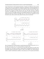
Some special simulation experiments were performed in order to validate the proposed
reinforcement learning control approach. Initial (starting) conditions of the simulation
examples (initial deviations of joints’ angles) were imposed. Simulation results were
analyzed on the time interval 0.1[s]. In the simulation example, two control algorithms were
analyzed: (i) basic dynamic controller described by computed torque method (without
learning) and (ii) hybrid reinforcement learning control algorithm. (with learning). The
results obtained by applying the controllers (i) (without learning) and (ii) (with learning) are
shown on Figs. 15 and Fig.16. It is evident , that better results were achieved with using
reinforcement learning control structure.
The corresponding position and velocity tracking erros in the case of application
reinforcement learning structure structure are presented on Figs. 17 and 18. The tracking
errirs converge to zero values in the given time interval. It means that the controller ensures
good tracking of the desired trajectory. Also, the application of reinforcement learning
structure ensures a dynamic balance of the locomotion mechanism
In Fig. 19 value of internal reinforcement through process of walking is presented. It is
clear that task of walking within desired ZMP tracking error limits is achieved in a good
fashion.
394 Humanoid Robots, New Developments
Fig. 13. Nominal joint angles of the right and left leg: q13, q17, q20, q24-roll, q14, q21, q16,
q18, q23, q25-pitch, q15, q22-yaw.
Reinforcement Learning Algorithms In Humanoid Robotics 395
Fig.14. Model-based animation of biped locomotion in several characteristic instants for the
experimentally determined joint trajectories.
0 10 20 30 40 50 60 70 80 90 100
-0.02
-0.015
-0.01
-0.005
0
0.005

0.01
0.015
Time (ms )
Error ZMP - x direction (m)
Fig. 15. Error of ZMP in x-direction (- with learning - . - without learning).
396 Humanoid Robots, New Developments
0 10 20 30 40 50 60 70 80 90 100
-0.02
-0.015
-0.01
-0.005
0
0.005
0.01
0.015
Time (m s)
Error ZMP - y direction (m)
Fig. 16. Error of ZMP in y-direction (- with learning - . - without learning).
0 10 20 30 40 50 60 70 80 90 100
-0.04
-0.03
-0.02
-0.01
0
0.01
0.02
0.03
0.04
Time (m s)
Position errors (rad)

Fig. 17. Position tracking errors.
0 10 20 30 40 50 60 70 80 90 100
-3
-2
-1
0
1
2
3
Time (ms )
Velocity errors (rad/s)
Fig. 18. Velocity tracking errors.
Reinforcement Learning Algorithms In Humanoid Robotics 397
0 10 20 30 40 50 60 70 80 90 100
-0.06
-0.04
-0.02
0
0.02
0.04
0.06
0.08
0.1
0.12
Reinforcement signal
Time (ms)
Fig. 19. Reinforcement through process of walking.
6. Conclusions
This study considers a optimal solutions for application of reinforcement learning in
humanoid robotics Humanoid Robotics is a very challenging domain for reinforcement

learning, Reinforcement learning control algorithms represents general framework to take
traditional robotics towards true autonomy and versatility. The reinforcement learning
paradigm described above has been successfully implemented for some special type of
humanoid robots in the last 10 years. Reinforcement learning is well suited to training biped
walk in particular teaching a robot a new behavior from scalar or fuzzy feedback. The
general goal in synthesis of reinforcement learning control algorithms is the development of
methods which scale into the dimensionality of humanoid robots and can generate actions
for biped with many degrees of freedom. In this study, control of walking of active and
passive dynamic walkers by using of reinforcement learning was amalyzed.
Various straightforward and hybrid intelligent control algorithms based RL for active and
passive biped locomotion is presented. The proposed RL algorithms use the learning
elements that consists of various types of neural networks, fuzzy logic nets or fuzzy-neuro
networks with focus on fast convergence properties and small number of learning trials.
Special part of study represents synthesis of hybrid intelligent controllers for biped walking.
The hybrid aspect is connected with application of model-based and model free approaches
as well as with combination of different paradigms of computational intelligence. These
algorithms includes combination of a dynamic controller based on dynamic model and
special compensators based on reinforcement structures. Two different reinforcement
learning structures were proposed based on actor-critic approach and Q-learning. The
algorithms is based on fuzzy evaluative feedback that are obtained from human intuitive
balancing knowledge. The reinforcement learning with fuzzy evaluation feedback is much
closer to the human biped walking evaluation than the original one with scalar feedback.
398 Humanoid Robots, New Developments
The proposed hybrid intelligent control scheme fulfills the preset control criteria. Its
application ensures the desired precision of robot’s motion, maintaining dynamic balance of
the locomotion mechanism during a motion
The developed hybrid intelligent dynamic controller can be potentially applied in
combination with robotic vision, to control biped locomotion mechanisms in the course of
fast walking, running, and even in the phases of jumping, as it possesses both the
conventional position-velocity feedback and dynamic reaction feedback. Performance of the

control system was analyzed in a number of simulation experiments in the presence of
different types of external and internal perturbations acting on the system. In this paper, we
only consider the flat terrain for biped walking. Because the real terrain is usually very
complex, more studies need to be conducted on the proposed gait synthesis method for
irregular and sloped terrain.
Dynamic bipedal walking is difficult to learn because combinatorial explosion in order to
optimize performance in every possible configuration of the robot., uncertainties of the
robot dynamics that must be only experimentally validated, and because coping with
dynamic discontinuities caused by collisions with the ground and with the problem of
delayed reward -torques applied at one time may have an effect on the performance many
steps into the future. Hence, for a physical robot, it is essential to learn from few trials in
order to have some time left for exploitation. It is thus necessary to speed the learning up by
using different methods (hierarchical learning, subtask decomposition, imitation,…).
7. Acknowledgments
The work described in this conducted was conducted within the national research project
”Dynamic and Control of High-Performance Humanoid Robots: Theory and Application”.
and was funded by the Ministry of Science and Environmental Protection of the Republic of
Serbia. The authors thank to Dr. Ing. Aleksandar Rodiþ for generation of experimental data
and realization of humanoid robot modeling and trajectory generation software.
8. References
Barto, A.G., Sutton, R.S & Anderson, C.W., (1983), Neuron like adaptive elements that can
solve difficult learning control problems, IEEE Transactions on Systems, Man,and
Cybernetics, SMC-13, 5, September 1983, 834–846.
Baxter, J. and Bartlett, P., (2001). Infinite-horizon policy-gradient estimation , Journal of
Artificial Intelligence Research, 319-350.
Benbrahim, H. & Franklin, J.A. (1997), Biped Dynamic Walking using Reinforcement
Learning, Robotics and Autonomous Systems, 22, 283-302.
Berenji,H.R. & Khedkar,P., (1992), Learning and Tuning Fuzzy Logic controllers through
Reinforcements, IEEE Transactions on Neural Networks, 724-740
Berenji, H.R., (1996), Fuzzy Q-learning for generalization of reinforcement,” in Proc. IEEE

Int. Conf. Fuzzy Systems, 2208–2214.
Bertsekas,D.P. and Tsitsiklis,J.N. (1996), Neuro-Dynamic Programming, Athena Scientific,
Belmont, USA.
Chew, C. & Pratt, G.A., (2002), Dynamic bipedal walking assisted by learning, Robotica, 477-491
Doya, K., (2000), Reinforcement Learning in Continuous Time and Space, Neural
Computation, 219-245.
Reinforcement Learning Algorithms In Humanoid Robotics 399
Glorennec, P.Y. & ouffe, L. (1997), Fuzzy Q – Learning, in Proceedings of FUZZ-IEEE’97,
Barcelona, July 1997.
Jouffe, L., (1998), Fuzzy inference system learning by reinforcement methods, IEEE Transactions
on Systems, Man, Cybernetics:Part C, Appl. Rev., 28, 3, August 1998, 338–355.
Kamio, S., & Iba, H., (2005), Adaptation Technique for Integrating Genetic Programming
and Reinforcement Learning fir Real Robot, IEEE Transactions on Evolutionary
Computation, 9, 3, June 2005, 318 - 333.
Katiþ, D. & Vukobratoviþ, M., (2003a), Survay of Intelligent Control Techniques for
Humanoid Robots, Journal of Intelligent and Robotic Systems, 37, 2003, 117 -141.
Katiþ, D. & Vukobratoviþ, M. (2003b), Intelligent Control of Robotic Systems, Kluwer Academic
Publishers, Dordrecht, Netherlands
Katiþ, D. & Vukobratoviþ, M.: (2005), Survey of Intelligent Control Algorithms For
Humanoid Robots”, in Proceedings of the 16th IFAC World Congress, Prague, Czech
Republic, July 2005.
Katiþ, D. & Vukobratoviþ, M., (2007), Hybrid Dynamic Control Algorithm for Humanoid
Robots Based on Reinforcement Learning, accepted for publication in Journal of
Intelligent and Robotic Systems .
Kimura, H. & Kobayashi, S. (1998), An analysis of actor/critic algorithms using eligibility
traces: Reinforcement learning with imperfect value functions ,in Proceedings of the
International Conference on Machine Learning (ICML ’98), 278-286.
Kun , A.L. and Miller,III, W.T., (1999), Control of Variable -Speed Gaits for a Biped Robot,
IEEE Robotics and Automation Magazine, 6, September 1999, 19-29.
Li, Q., Takanishi, A. & Kato, I., (1992), Learning control of compensative trunk motion for

biped walking robot based on ZMP, in Proceedings of the 1992 IEEE/RSJ
Intl.Conference on Intelligent Robot and Systems, 597–603.
Mori, T., Nakamura, Y., Sato, M. and Ishii, S., (2004), Reinforcement learning for a cpg-
driven biped robot, in Proceedings of the Nineteenth National Conference on Artificial
Intelligence (AAAI), 623–630.
Morimoto, J., Cheng, G., Atkeson, C.G. & Zeglin,G., (2004) A Simple Reinforcement
Learning Algorithm For Biped Walking, in Proceedings of the 2004 IEEE International
Conference on Robotics & Automation, New Orleans, USA.
Nagasaka, K., Inoe, H. and Inaba, M., (1999), Dynamic walking pattern generation for a
humanoid robot based on optimal gradient method, in Proceedings of the
International Conference on Systems, Man. and Cybernetics, 908-913.
Nakamura, Y., Sato, M. & Ishii, S., (2003), Reinforcement learning for biped robot, in Proceedings
of the 2nd International Symposium on Adaptive Motion of Animals and Machines.
Peters, J., Vijayakumar, S., and Schaal, S., (2003), Reinforcement Learning for Humanoid
Robots, in Proceedings of the Third IEEE-RAS International Conference on Humanoid
Robots, Karlsruhe & Munich.
Rodi
þ, A., Vukobratoviþ, M., Addi, K. & Dalleau, G. (2006), Contribution to the Modelling of
Non-Smooth, Multi-Point Contact Dynamcs of Biped Locomotion – Theory and
Experiments, submitted to journal Robotica.
Salatian, A.W., Yi, K.Y. and Zheng, Y.F., (1997) , Reinforcement Learning for a Biped Robot
to Climb Sloping Surfaces, Journal of Robotic Systems, 283-296.
Schuitema, E., Hobbelen, D G.E, Jonker, P.P., Wisse, M. & Karssen, J.G.D., (2005), Using a
controller based on reinforcement learning for a passive dynamic walking robot,
IEEE International conference on Humanoid Robots 2005, Tsukuba, Japan.
400 Humanoid Robots, New Developments
Sutton, R.S. and Barto,A.G. (1998) Reinforcement Learning: An Introduction, The MIT Press,
Cambridge, USA.
Sutton, R.S., McAllester, D., & Singh, S., (2000), Policy Gradient Methods for Reinforcement
learning with Function Approximation, in Advances in Neural Information Processing

Systems, 12, MIT Press, Cambrdige, USA, 1057-1063.
Tedrake, R.,Zhang, T.W. & Seung, H.S., (2004), Stochastic policy gradient reinforcement
learning on a simple 3d biped, in Proceedings of the 2004 IEEE/RSJ International
Conference on Intelligent Robots and Systems.
Vukobratoviþ, M, & JuriĀiþ, D. (1969), Contribution to the Synthesis of Biped Gait, IEEE
Transactions on Biomedical Engineering, BME-16, 1, 1-6.
Vukobratoviþ, M., Borovac, B., Surla, D., & Stokiþ, D., (1990), Biped Locomotion - Dynamics,
Stability, Control and Application, Springer Verlag, Berlin, Germany.
Watkins, C.J.C.H. & Dayan, P., (1992), Q Learning, Machine Learning,, 279-292.
Zatsiorsky, V., Seluyanov, V. & Chugunova, L. (1990) ,Methods of Determining Mass –
Inertial Characteristics of Human Body Segments, Contemporary Problems of
Biomechanics, 272-291, CRC Press
.
Zhou, C. & Meng, D. (2000), Reinforcement Learning with Fuzzy Evaluative Feedback for a
Biped Robot. In:Proceedings of the IEEE International Conference on Robotics and
Automation, San Francisko, USA, 3829-3834.
23
A Designing of Humanoid Robot Hands in Endo
skeleton and Exoskeleton Styles
Ichiro Kawabuchi
KAWABUCHI Mechanical Engineering Laboratory, Inc.
Japan
1. Introduction
For a serious scientific interest or rather an amusing desire to be the creator like Pygmalion,
human being has kept fascination to create something replicates ourselves as shown in
lifelike statues and imaginative descriptions in fairy tales, long time from the ancient days.
At the present day, eventually, they are coming out as humanoid robots and their brilliant
futures are forecasted as follows. 1) Humanoid robot will take over boring recurrent jobs
and dangerous tasks where some everyday tools and environments designed and optimised
for human usage should be exploited without significant modifications. 2) Efforts of

developing humanoid robot systems and components will lead some excellent inventions of
engineering, product and service. 3) Humanoid robot will be a research tool by itself for
simulation, implementation and examination of the human algorithm of motions,
behaviours and cognitions with corporeality.
At the same time, I cannot help having some doubts about the future of the humanoid robot
as extension of present development style. Our biological constitution is evolved properly to
be made of bio-materials and actuated by muscles, and present humanoid robots, on the
contrary, are bounded to be designed within conventional mechanical and electric elements
prepared for industrial use such as electric motors, devices, metal and plastic parts. Such
elements are vastly different in characteristics from the biological ones and are low in some
significant properties: power/weight ratio, minuteness, flexibility, robustness with self-
repairing, energy and economic efficiency and so on. So the “eternal differences” in function
and appearance will remain between the human and the humanoid robots.
I guess there are chiefly two considerable ways for developing a preferable humanoid robot
body. One is to promote in advance a development of artificial muscle that is exactly similar
to the biological one. It may be obvious that an ideal humanoid robot body will be
constructed by a scheme of putting a skeletal model core and attaching the perfect artificial
muscles on it (Weghel et al., 2004, e.g.). Another is to establish some practical and realistic
designing paradigms within extensional technology, in consideration of the limited
performance of mechanical and electric elements. In this way, it will be the key point that
making full use of flexible ideas of trimming and restructuring functions on a target. For
example, that is to make up an alternative function by integrating some simple methods,
when the target function is too complex to be a unitary package. Since it seems to take long
time until the complete artificial muscles will come out, I regard the latter way is a good
prospect to the near future rather than just a compromise.