Industrial Robotics Theory Modelling and Control Part 3 pot
Bạn đang xem bản rút gọn của tài liệu. Xem và tải ngay bản đầy đủ của tài liệu tại đây (490.37 KB, 60 trang )
Kinematic design and description of industrial robotic chains 109
kinematic graph contour molecule
ǂǃǂƦ−−−
mechanism robot
Figure 9. Mitsubishi Electric robot
5.2.5 Robot with a main structure having two degrees of mobility and I=2
The starting point for generating of the kinematic structure is the first logical
equation of Table 7 (Watt's structure). For the desired robot, the G
1,6
structure
thus obtained lacks one degree of mobility and five links. The following opera-
tions allow its completion (cf. fig. 10). Adding to this structure a frame and an
end-effector the resulting mechanism of this operation corresponds to the main
structure of the level 4 HPR Andromat robot.
stage/ logical equati-
on
kinematic graph contour molecule
first: addition of three
links and one de
g
ree
of mobility
9,23,16,1 G
A
G =+
DŽǂǂƧ−−−
second: addition of
two links
11,22,09,2 G
A
G =+
adopted solution
ǂDŽǂDŽƧ−−−−
α
γ
γ
α
Ε
γ
α
α
Ε
α
Δ
α
β
110 Industrial Robotics: Theory, Modelling and Control
mechanism robot
Figure 10. Evolution of the generation of the Andromat robot topological chain
(source:
Among the one hundred and ten available structures of type G
2,11
, a robot
manufacturer has implemented the required solution above in order to design
the main structure of the Andromat robot. According to the rules defined in §
3.1.2. the frame, initially a quaternary link, was transformed into a quintarny
one and the binary link, where the end-effector was attached, into a ternary
one.
This robot is equipped with a pantographic system with a working range of 2,5
m and weight range from 250 kg up to 2000 kg. The Andromat is a world-
renowned manipulator, which is widely and successfully used in foundry and
forging industries enabling operators to lift and manipulate heavy and awk-
ward components in hostile and dangerous environments. (source:
/>During the initial design of the MS of robots, the validation of their topological
structures may be done by studying the kinematic graphs of their main struc-
tures. The representation by molecules mainly yields to the usual structural
diagram of the mechanism in order to visualise and simplify. This allows the
classification of their structures and their assignation to different classes of
structures, taking into account of their complexity expressed by the number of
closed loops. Those points are the subject of the next paragraph.
Kinematic design and description of industrial robotic chains 111
6. Classification of industrial robots structures
The structures of robots with simple kinematic chains may be represented by one
open kinematic structures of type A. We call these open structures 0 (zero)
level structures. Many industrial robots are of the same type for example: MA
23 Arm, SCARA carrier, AID-5V, Seiko 700, Versatran Vertical 80, Puma 500,
Kawasaki Js-2, Toshiba SR-854HSP and Yamaha robots (Ferreti, 1981; Rob-Aut,
1996).
The main structures of robots with closed kinematic chains may be represented
by closed kinematic chains of type G derived from MMT. The Pick and Place
robot, for instance, has only one closed chain. This is a level 1 (one) robot (cf. §
5.2.1). There are other industrial robots of the same level for example: Tokico,
Pana-Robo by Panasonic, SK 16 and SK 120 by Yaskawa, SC 35 Nachi etc (Rob-
Aut, 1996).
The main structure of the AKR-3000 robot is composed of two closed loops
represented by two internal contours in its molecule. This is a level 2 (two) ro-
bot. The main structure of Moise-Pelecudi robot (Manolescu et al, 1987) is
composed of three closed chains defining a level 3 (three) robot. The main
structure of the Andromat robot is composed of four closed chains. This is a
level 4 (four) robot etc. Hence the level n of a robot is defined by the number n
of internal contours in its molecule. Table 16 completes this classification of
certain robots presented by Ferreti in (Ferreti, 1981):
robot manufacturer main struc-
ture of the
robot
contour nb. of
internal
contour
s
level
Nordson
Robomatic
Nordson
France
Binks
Manufacturing
Co.
-
(simple chain)
0
0
zero
zero
Cincinnati
T3, HT3
HPR- Hita-
chi
Cincinnati
Milacron Fran-
ce
ǂƣ−
ǃ
Ƥ−
1
1
one
one
RASN AOIP Kremlin,
Robotique
AKR
ǃ
ǂƦ−−
2 two
112 Industrial Robotics: Theory, Modelling and Control
AS50VS Mitsubishi
Electric/ Japan
ǂǃǂƦ−−−
3 three
Andromat …/Sweden
ǂDŽǂDŽ−−−
−
4 four
Table 16. Levels of different industrial robots
7. Conclusions and Future Plans
In this chapter we presented an overview about the chronology of design
process of an industrial robot kinematic chain. The method for symbolical syn-
thesis of planar link mechanisms in robotics presented here allows the genera-
tion of plane mechanical structures with different degrees of mobility. Based
on the notion of logical equations, this enables the same structures obtained us-
ing different methods to be found (intuitive methods, Assur's groups, trans-
formation of binary chains etc).
The goal being to represent the complexity of the topological structure of an
industrial robot, a new method for description of mechanisms was proposed.
It is based on the notions of contours and molecules. Its advantage, during the
initial phase of the design of the robots, is that the validation of their topologi-
cal structures can be done by comparing their respective molecules. That
makes it possible to reduce their number by eliminating those which are iso-
morphic.
The proposed method is afterwards applied for the description of closed struc-
tures derived from MMT for different degrees of mobility. It is then applied to
the description and to the classification of the main structures of different in-
dustrial robots. The proposed method permits the simplification of the visuali-
sation of their topological structures. Finally a classification of industrial robots
of different levels taking into account the number of closed loops in their
molecules is presented.
In addition to the geometrical, kinematical and dynamic performances, the de-
sign of a mechanical system supposes to take into account, the constraints of
the kinematic chain according to the:
- position of the frame,
- position of the end-effector,
- and position of the actuators.
The two first aspects above are currently the subjects of our research. The
problem is how to choose among the possible structures provided by MMT ac-
Kinematic design and description of industrial robotic chains 113
cording to the position of the frame and the end-effector. As there may be a
large number of these mechanisms, it is usually difficult to make a choice
among the available structures in the initial design phase of the robot chain. In
fact, taking into account the symmetries it can be noticed that there are a sig-
nificant number of isomorphic structures according to the position of the
frame and of the end-effector of the robot. Our future objectives are:
- to find planar mechanisms with revolute joints that provide guidance of
a moving frame, e.g. the end-effector of an industrial robot, relative to a
base frame with a given degree of freedom,
- to reduce the number of kinematic structures provided by MMT, which
are suitable for robotics applications, taking into account the symme-
tries the two criteria being the position of the frame and of the end-
effector of the robot.
114 Industrial Robotics: Theory, Modelling and Control
8. References
Abo-Hammour, Z.S.; Mirza, N.M.; Mirza, S.A. & Arif, M. (2002). Cartesian
path generation of robot manipulators continuous genetic algorithms,
Robotics and autonomous systems. Dec 31, 41 (4), pp.179-223.
Artobolevski, I. (1977). Théorie des mécanismes, Mir, Moscou.
Belfiore, N.P. (2000). Distributed databases for the development of mecha-
nisms topology, Mechanism and Machine Theory Vol. 35, pp. 1727-1744.
Borel, P. (1979). Modèle de comportement des manipulateurs. Application à l’analyse
de leurs performances et à leur commande automatique, PhD Thesis, Mont-
pellier.
Cabrera, J.A.; Simon, A. & Prado, M. (2002). Optimal synthesis of mechanisms
with genetic algorithms, Mechanism and Machine Theory, Vol. 37, pp.
1165-1177.
Coiffet, P. (1992). La robotique. Principes et applications, Hermès, Paris.
Crossley, F. R. E. (1964). A cotribution to Grubler's theory in the number syn-
thesis of plane mechanisms, Transactions of the ASME, Journal of Engi-
neering for Industry, 1-8.
Crossley, F.R.E. (1966). On an unpublished work of Alt, Journal of Mecha-
nisms, 1, 165-170.
Davies, T. & Crossley, F.R.E. (1966). Structural analysis of plan linkages by
Franke’s condensed notation, Pergamon Press, Journal of Mechanisms,
Vol., 1, 171-183.
Dobrjanskyi L., Freudenstein F., 1967. Some application of graph theory to the
structural analysis of mechanisms, Transactions of the ASME, Journal of
Engineering for Industry, 153-158.
Erdman A., Sandor G. N., 1991. Mechanism Design, Analysis and Synthesis, Sec-
ond edition.
Ferreti, M. (1981). Panorama de 150 manipulateurs et robots industriels, Le
Nouvel Automatisme, Vol., 26, Novembre-Décembre, 56-77.
Gonzales-Palacois, M. & Ahjeles J. (1996). USyCaMs : A software Package for
the Interactive Synthesysis of Cam Mecanisms, Proc. 1-st Integrated De-
sign end Manufacturing in Mechanical Engineering I.D.M.M.E.'96, Nantes
France, 1, 485-494.
Hervé L M., 1994. The mathematical group structure of the set of displace-
ments, Mech. and Mach. Theory, Vol. 29, N° 1, 73-81.
Hwang, W-M. & Hwang, Y-W. (1992). Computer-aided structural synthesis of
plan kinematic chains with simple joints Mechanism and Machine Theory,
27, N°2, 189-199.
Karouia, M. & Hervè, J.M. (2005). Asymmetrical 3-dof spherical parallel
mechanisms, European Journal of Mechanics (A/Solids), N°24, pp.47-57.
Kinematic design and description of industrial robotic chains 115
Khalil, W. (1976). Modélisation et commande par calculateur du manipulateur MA-
23. Extension à la conception par ordinateur des manipulateurs, PhD Thesis.
Montpellier.
Laribi, M.A. ; Mlika, A. ; Romdhane, L. & Zeghloul, S. (2004). A combined ge-
netic algorithm-fuzzy logic method (GA-FL) in mechanisms synthesis,
Mechanism and Machine Theory 39, pp. 717-735.
Ma, O. & Angeles, J. (1991). Optimum Architecture Design of Platform Ma-
nipulators, IEEE, 1130-1135.
Manolescu, N. (1964). Une méthode unitaire pour la formation des chaînes ci-
nématiques et des mécanismes plans articulés avec différents degrés de
liberté et mobilité, Revue Roumaine Sciances. Techniques- Mécanique Appli-
quée, 9, N°6, Bucarest, 1263-1313.
Manolescu, N. ; Kovacs, F.R. & Oranescu, A. (1972). Teoria Mecanismelor si a
masinelor, Editura didactica si pedagogica, Bucuresti.
Manolescu, N (1979). A unified method for the formation of all planar joined
kinematic chains and Baranov trusses, Environment and Planning B, 6,
447-454.
Manolescu, N. ; Tudosie, I. ; Balanescu, I. ; Burciu, D. & Ionescu, T. (1987).
Structural and Kinematic Synthesis of Planar Kinematic Chain (PKC)
and Mechanisms (PM) with Variable Structure During the Work, Proc. of
the 7-th World Congress, The Theory of Machines and Mechanisms, 1, Sevilla,
Spain, 45-48.
Manolescu N., 1987. Sur la structure des mécanismes en robotique, Conférence
à l’Ecole centrale d’Arts et Manufactures, Paris 1987.
Merlet, J P. (1996). Workspace-oriented methodology for designing a parallel
manipulator ", Proc. 1-st Integrated Design end Manufacturing in Mechani-
cal Engineering I.D.M.M.E.'96, April 15-17, Nantes France, Tome 2, 777-
786.
Mitrouchev, P. & André, P. (1999). Méthode de génération et description de
mécanismes cinématiques plans en robotique, Journal Européen des Sys-
tèmes Automatisés, 33(3), 285-304.
Mitrouchev, P. (2001). Symbolic structural synthesis and a description method
for planar kinematic chains in robotics, European Journal of Mechanics (A
Solids), N°20, pp.777-794.
Mruthyunjaya, T.S. (1979). Structural Synthesis by Transformation of Binary
Chains, Mechanism and Machine Theory, 14, 221-238.
Mruthyunjaya, T.S. (1984-a). A computerized methodology for structural syn-
thesis of kinematic chains: Part 1- Formulation, Mechanism and Machine
Theory, 19, No.6, 487-495.
Mruthyunjaya, T.S. (1984-b). A computerized methodology for structural syn-
thesis of kinematic chains: Part 2-Application to several fully or par-
tially known cases, Mechanism and Machine Theory, 19, No.6, 497-505.
116 Industrial Robotics: Theory, Modelling and Control
Mruthyunjaya, T.S. (1984-c). A computerized methodology for structural syn-
thesis of kinematic chains: Part 3-Application to the new case of 10-link,
three-freedom chains, Mechanism and Machine Theory, 19, No.6, 507-530.
Pieper, L. & Roth, B. (1969). The Kinematics of Manipulators Under Computer
Control, Proceedings 2-nd International Congress on The Theory of Machines
and Mechanisms, 2, 159-168.
Rao, A. C. & Deshmukh, P. B. (2001). Computer aided structural synthesis of
planar kinematic chains obviating the test for isomorphism, Mechanism
and Machine Theory 36, pp. 489-506.
Renaud, M. (1975). Contribution à l’étude de la modélisation et de la commande des
systèmes mécaniques articulés, Thèse de Docteur ingénieur. Université
Paul Sabatier, Toulouse.
Rob-Aut. (1996). La robotique au Japon, ROBotisation et AUTomatisation de la
production, N°12, Janvier-Février, 28-32.
Roth, B. (1976). Performance Evaluation of manipulators from a kinamatic
viewpoint, Cours de robotique. 1, IRIA.
Tejomurtula, S. & Kak, S. (1999). Inverse kinematics in robotics using neural
networks, Information sciences, 116 (2-4), pp. 147-164.
Tischler, C. R.; Samuel A. E. & Hunt K. H. (1995). Kinematic chains for robot
hands – I. Orderly number-synthesis, Mechanism and Machine Theory, 30,
No.8, pp. 1193-1215.
Touron, P. (1984). Modélisation de la dynamique des mécanismes polyarticu-
lés. Application à la CAO et à la simulation de robots, Thèse, Université de
Montpellier.
Warneke, H.J. (1977). Research activities and the I.P.A. in the field of robotics,
Proc. of the 7-th ISIR Congress, Tokyo, 25-35.
Woo, L. S. (1967). Type synthesis of plan linkages, Transactions of the ASME,
Journal of Engineering for Industry, 159-172.
117
4
Robot Kinematics:
Forward and Inverse Kinematics
Serdar Kucuk and Zafer Bingul
1. Introduction
Kinematics studies the motion of bodies without consideration of the forces or
moments that cause the motion. Robot kinematics refers the analytical study of
the motion of a robot manipulator. Formulating the suitable kinematics mod-
els for a robot mechanism is very crucial for analyzing the behaviour of indus-
trial manipulators. There are mainly two different spaces used in kinematics
modelling of manipulators namely, Cartesian space and Quaternion space. The
transformation between two Cartesian coordinate systems can be decomposed
into a rotation and a translation. There are many ways to represent rotation,
including the following: Euler angles, Gibbs vector, Cayley-Klein parameters,
Pauli spin matrices, axis and angle, orthonormal matrices, and Hamilton 's
quaternions. Of these representations, homogenous transformations based on
4x4 real matrices (orthonormal matrices) have been used most often in robot-
ics. Denavit & Hartenberg (1955) showed that a general transformation be-
tween two joints requires four parameters. These parameters known as the
Denavit-Hartenberg (DH) parameters have become the standard for describing
robot kinematics. Although quaternions constitute an elegant representation
for rotation, they have not been used as much as homogenous transformations
by the robotics community. Dual quaternion can present rotation and transla-
tion in a compact form of transformation vector, simultaneously. While the
orientation of a body is represented nine elements in homogenous transforma-
tions, the dual quaternions reduce the number of elements to four. It offers
considerable advantage in terms of computational robustness and storage effi-
ciency for dealing with the kinematics of robot chains (Funda et al., 1990).
The robot kinematics can be divided into forward kinematics and inverse
kinematics. Forward kinematics problem is straightforward and there is no
complexity deriving the equations. Hence, there is always a forward kinemat-
ics solution of a manipulator. Inverse kinematics is a much more difficult prob-
lem than forward kinematics. The solution of the inverse kinematics problem
is computationally expansive and generally takes a very long time in the real
time control of manipulators. Singularities and nonlinearities that make the
118 Industrial Robotics: Theory, Modelling and Control
problem more difficult to solve. Hence, only for a very small class of kinemati-
cally simple manipulators (manipulators with Euler wrist) have complete ana-
lytical solutions (Kucuk & Bingul, 2004). The relationship between forward
and inverse kinematics is illustrated in Figure 1.
T
n
θ
1
Forward kinematics
Inverse kinematics
Cartesian
space
Joint
space
θ
2
θ
n
0
.
Figure 10. The schematic representation of forward and inverse kinematics.
Two main solution techniques for the inverse kinematics problem are analyti-
cal and numerical methods. In the first type, the joint variables are solved ana-
lytically according to given configuration data. In the second type of solution,
the joint variables are obtained based on the numerical techniques. In this
chapter, the analytical solution of the manipulators is examined rather then
numerical solution.
There are two approaches in analytical method: geometric and algebraic solu-
tions. Geometric approach is applied to the simple robot structures, such as 2-
DOF planar manipulator or less DOF manipulator with parallel joint axes. For
the manipulators with more links and whose arms extend into 3 dimensions or
more the geometry gets much more tedious. In this case, algebraic approach is
more beneficial for the inverse kinematics solution.
There are some difficulties to solve the inverse kinematics problem when the
kinematics equations are coupled, and multiple solutions and singularities ex-
ist. Mathematical solutions for inverse kinematics problem may not always
correspond to the physical solutions and method of its solution depends on the
robot structure.
This chapter is organized in the following manner. In the first section, the for-
ward and inverse kinematics transformations for an open kinematics chain are
described based on the homogenous transformation. Secondly, geometric and
algebraic approaches are given with explanatory examples. Thirdly, the prob-
lems in the inverse kinematics are explained with the illustrative examples. Fi-
nally, the forward and inverse kinematics transformations are derived based
on the quaternion modeling convention.
Robot Kinematics: Forward and Inverse Kinematics 119
2. Homogenous Transformation Modelling Convention
2.1. Forward Kinematics
A manipulator is composed of serial links which are affixed to each other revo-
lute or prismatic joints from the base frame through the end-effector. Calculat-
ing the position and orientation of the end-effector in terms of the joint vari-
ables is called as forward kinematics. In order to have forward kinematics for a
robot mechanism in a systematic manner, one should use a suitable kinematics
model. Denavit-Hartenberg method that uses four parameters is the most
common method for describing the robot kinematics. These parameters a
i-1
,
1i−
α , d
i
and θ
i
are the link length, link twist, link offset and joint angle, respec-
tively. A coordinate frame is attached to each joint to determine DH parame-
ters. Z
i
axis of the coordinate frame is pointing along the rotary or sliding di-
rection of the joints. Figure 2 shows the coordinate frame assignment for a
general manipulator.
1i−
α
Link i-1
Y
i-1
Z
i-1
X
i-1
a
i-1
d
i
Y
i
Z
i
X
i
θ
i
Link i
a
i
Y
i+1
Z
i+1
X
i+1
Figure 2. Coordinate frame assignment for a general manipulator.
As shown in Figure 2, the distance from Z
i-1
to Z
i
measured along X
i-1
is as-
signed as a
i-1
, the angle between Z
i-1
and Z
i
measured along X
i
is assigned as
α
i-1
, the distance from X
i-1
to X
i
measured along Z
i
is assigned as d
i
and the an-
gle between X
i-1
to X
i
measured about Z
i
is assigned as θ
i
(Craig, 1989).
The general transformation matrix T
1i
i
−
for a single link can be obtained as fol-
lows.
120 Industrial Robotics: Theory, Modelling and Control
()()()()
iiiz1ix1ix
1i
i
dQRaDRT θα=
−−
−
»
»
»
»
¼
º
«
«
«
«
¬
ª
»
»
»
»
¼
º
«
«
«
«
¬
ª
θθ
θ−θ
»
»
»
»
¼
º
«
«
«
«
¬
ª
»
»
»
»
¼
º
«
«
«
«
¬
ª
αα
α−α
=
−
−−
−−
1000
d100
0010
0001
1000
0100
00cs
00sc
1000
0100
0010
a001
1000
0cs0
0sc0
0001
i
ii
ii1i
1i1i
1i1i
»
»
»
»
¼
º
«
«
«
«
¬
ª
αααθαθ
α−α−αθαθ
θ−θ
=
−−−−
−−−−
−
1000
dccscss
dsscccs
a0sc
i1i1i1ii1ii
i1i1i1ii1ii
1iii
(1)
where R
x
and R
z
present rotation, D
x
and Q
i
denote translation, and cθ
i
and
sθ
i
are the short hands of cosθ
i
and sinθ
i
, respectively. The forward kinematics
of the end-effector with respect to the base frame is determined by multiplying
all of the T
1i
i
−
matrices.
T TTT
1n
n
1
2
0
1
base
effector_end
−
=
(2)
An alternative representation of
T
base
effector_end
can be written as
»
»
»
»
¼
º
«
«
«
«
¬
ª
=
−
1000
prrr
prrr
prrr
T
z333231
y232221
x131211
base
effectorend
(3)
where r
kj
’s represent the rotational elements of transformation matrix (k and
j=1, 2 and 3). p
x
, p
y
and p
z
denote the elements of the position vector. For a six
jointed manipulator, the position and orientation of the end-effector with re-
spect to the base is given by
)q(T)q(T)q(T)q(T)q(T)q(TT
6
5
65
4
54
3
43
2
32
1
21
0
1
0
6
= (4)
where q
i
is the joint variable (revolute or prismatic joint) for joint i, (i=1, 2,
.6).
Robot Kinematics: Forward and Inverse Kinematics 121
Example 1.
As an example, consider a 6-DOF manipulator (Stanford Manipulator) whose
rigid body and coordinate frame assignment are illustrated in Figure 3. Note
that the manipulator has an Euler wrist whose three axes intersect at a com-
mon point. The first (RRP) and last three (RRR) joints are spherical in shape. P
and R denote prismatic and revolute joints, respectively. The DH parameters
corresponding to this manipulator are shown in Table 1.
z
0,1
y
2
x
2
z
2
z
0
y
0
d
3
y
3
z
3
x
3
θ
1
θ
2
x
0
z
1
y
1
x
1
h
1
d
2
θ
4
θ
5
θ
6
z
4
x
4
y
4
z
5
x
5
y
5
z
6
x
6
y
6
Figure 3. Rigid body and coordinate frame assignment for the Stanford Manipulator.
i
θ
i
α
i-1
a
i-1
d
i
1
θ
1
0 0 h
1
2
θ
2
90 0 d
2
3 0 -90 0 d
3
4
θ
4
0 0 0
5
θ
5
90 0 0
6
θ
6
-90 0 0
Table 1. DH parameters for the Stanford Manipulator.
122 Industrial Robotics: Theory, Modelling and Control
It is straightforward to compute each of the link transformation matrices using
equation 1, as follows.
»
»
»
»
¼
º
«
«
«
«
¬
ª
θθ
θ−θ
=
1000
h100
00cs
00sc
T
1
11
11
0
1
(5)
»
»
»
»
¼
º
«
«
«
«
¬
ª
θθ
−−
θ−θ
=
1000
00cs
d100
00sc
T
22
2
22
1
2
(6)
»
»
»
»
¼
º
«
«
«
«
¬
ª
−
=
1000
0010
d100
0001
T
3
2
3
(7)
»
»
»
»
¼
º
«
«
«
«
¬
ª
θθ
θ−θ
=
1000
0100
00cs
00sc
T
44
44
3
4
(8)
»
»
»
»
¼
º
«
«
«
«
¬
ª
θθ
−
θ−θ
=
1000
00cs
0100
00sc
T
55
55
4
5
(9)
»
»
»
»
¼
º
«
«
«
«
¬
ª
θ−θ−
θ−θ
=
1000
00cs
0100
00sc
T
66
66
5
6
(10)
The forward kinematics of the Stanford Manipulator can be determined in the
form of equation 3 multiplying all of the
T
1i
i
−
matrices, where i=1,2, …, 6. In
this case, T
0
6
is given by
Robot Kinematics: Forward and Inverse Kinematics 123
»
»
»
»
¼
º
«
«
«
«
¬
ª
=
1000
prrr
prrr
prrr
T
z333231
y232221
x131211
0
6
(11)
where
)ssc)cccss(c(c)sccsc(sr
521421415642114611
θθθ+θθθ−θθθθ−θθθ+θθθ−=
)sccsc(c)ssc)cccss(c(sr
421146521421415612
θθθ+θθθ−θθθ+θθθ−θθθθ=
25142141513
scc)cccss(sr θθθ−θθθ−θθθ=
)sss)sccsc(c(c)ssccc(sr
521142415641241621
θθθ−θθθ+θθθθ+θθθ−θθθ=
)sss)sccsc(c(s)ssccc(cr
521142415641241622
θθθ−θθθ+θθθθ−θθθ−θθθ=
21514241523
ssc)sccsc(sr θθθ−θθθ+θθθ−=
64225452631
sss)sccsc(cr θθθ−θθθ+θθθ=
42625452632
ssc)sccsc(sr θθθ−θθθ+θθθ−=
5245233
sscccr θθθ−θθ=
21312x
scdsdp θθ−θ=
21312y
ssdcdp θθ−θ−=
231z
cdhp θ+=
2.1.1 Verification of Mathematical model
In order to check the accuracy of the mathematical model of the Stanford Ma-
nipulator shown in Figure 3, the following steps should be taken. The general
position vector in equation 11 should be compared with the zero position vec-
tor in Figure 4.
124 Industrial Robotics: Theory, Modelling and Control
z
0,1
h
1
d
2
d
3
+z
0
+y
0
+x
0
-x
0
-y
0
Figure 4. Zero position for the Stanford Manipulator.
The general position vector of the Stanford Manipulator is given by
»
»
»
¼
º
«
«
«
¬
ª
θ+
θθ−θ−
θθ−θ
=
»
»
»
¼
º
«
«
«
¬
ª
231
21312
21312
z
y
x
cdh
ssdcd
scdsd
p
p
p
(12)
In order to obtain the zero position in terms of link parameters, let’s set
θ
1
=θ
2
=0
°
in equation 12.
»
»
»
¼
º
«
«
«
¬
ª
+
−=
»
»
»
¼
º
«
«
«
¬
ª
+
−−
−
=
»
»
»
¼
º
«
«
«
¬
ª
31
2
31
32
32
z
y
x
dh
d
0
)0(cdh
)0(s)0(sd)0(cd
)0(s)0(cd)0(sd
p
p
p
$
$$$
$$$
(13)
All of the coordinate frames in Figure 3 are removed except the base which is
the reference coordinate frame for determining the link parameters in zero po-
sition as in Figure 4. Since there is not any link parameters observed in the di-
rection of +x
0
and -x
0
in Figure 4, p
x
=0. There is only d
2
parameter in –y
0
direc-
tion so p
y
equals -d
2
. The parameters h
1
and d
3
are the +z
0
direction, so p
z
equals h
1
+d
3
. In this case, the zero position vector of Stanford Manipulator are
obtained as following
Robot Kinematics: Forward and Inverse Kinematics 125
»
»
»
¼
º
«
«
«
¬
ª
+
−=
»
»
»
¼
º
«
«
«
¬
ª
31
2
z
y
x
dh
d
0
p
p
p
(14)
It is explained above that the results of the position vector in equation 13 are
identical to those obtained by equation 14. Hence, it can be said that the
mathematical model of the Stanford Manipulator is driven correctly.
2.2. Inverse Kinematics
The inverse kinematics problem of the serial manipulators has been studied
for many decades. It is needed in the control of manipulators. Solving the in-
verse kinematics is computationally expansive and generally takes a very long
time in the real time control of manipulators. Tasks to be performed by a ma-
nipulator are in the Cartesian space, whereas actuators work in joint space.
Cartesian space includes orientation matrix and position vector. However,
joint space is represented by joint angles. The conversion of the position and
orientation of a manipulator end-effector from Cartesian space to joint space is
called as inverse kinematics problem. There are two solutions approaches
namely, geometric and algebraic used for deriving the inverse kinematics solu-
tion, analytically. Let’s start with geometric approach.
2.2.1 Geometric Solution Approach
Geometric solution approach is based on decomposing the spatial geometry of
the manipulator into several plane geometry problems.It is applied to the sim-
ple robot structures, such as, 2-DOF planer manipulator whose joints are both
revolute and link lengths are l
1
and l
2
shown in Figure 5a. Consider Figure 5b
in order to derive the kinematics equations for the planar manipulator.
The components of the point P (p
x
and p
y
) are determined as follows.
126 Industrial Robotics: Theory, Modelling and Control
l
1
θ
1
θ
2
l
2
X
Y
P
(a)
Y
θ
2
θ
1
θ
1
l
1
l
2
X
l
1
cos
θ
1
l
2
cos
(θ
1
+
θ
2
)
l
1
sin
θ
1
l
2
sin
(θ
1
+
θ
2
)
P
(b)
Figure 5. a) Planer manipulator; b) Solving the inverse kinematics based on trigo-
nometry.
12211x
clclp θ+θ= (15)
12211y
slslp θ+θ= (16)
where
212112
ssccc θθ−θθ=θ and
212112
sccss θθ+θθ=θ . The solution of
2
θ can be
computed from summation of squaring both equations 15 and 16.
1212112
22
21
22
1
2
x
ccll2clclp θθ+θ+θ=
1212112
22
21
22
1
2
y
ssll2slslp θθ+θ+θ=
)sscc(ll2)sc(l)sc(lpp
1211212112
2
12
22
21
2
1
22
1
2
y
2
x
θθ+θθ+θ+θ+θ+θ=+
Robot Kinematics: Forward and Inverse Kinematics 127
Since 1sc
1
2
1
2
=θ+θ , the equation given above is simplified as follows.
])sccs[s]sscc[c(ll2llpp
212112121121
2
2
2
1
2
y
2
x
θθ+θθθ+θθ−θθθ++=+
)ssccsssccc(ll2llpp
21121
2
21121
2
21
2
2
2
1
2
y
2
x
θθθ+θθ+θθθ−θθ++=+
])sc[c(ll2llpp
1
2
1
2
221
2
2
2
1
2
y
2
x
θ+θθ++=+
221
2
2
2
1
2
y
2
x
cll2llpp θ++=+
and so
21
2
2
2
1
2
y
2
x
2
ll2
llpp
c
−−+
=θ
(17)
Since,
1sc
i
2
i
2
=θ+θ (i =1,2,3,……),
2
sθ is obtained as
2
21
2
2
2
1
2
y
2
x
2
ll2
llpp
1s
¸
¸
¹
·
¨
¨
©
§
−−+
−±=θ
(18)
Finally, two possible solutions for
2
θ can be written as
¸
¸
¹
·
¨
¨
©
§
−−+
¸
¸
¹
·
¨
¨
©
§
−−+
−±=θ
21
2
2
2
1
2
y
2
x
2
21
2
2
2
1
2
y
2
x
2
ll2
llpp
,
ll2
llpp
12tanA
(19)
Let’s first, multiply each side of equation 15 by
1
cθ and equation 16 by
1
sθ and
add the resulting equations in order to find the solution of
1
θ in terms of link
parameters and the known variable
2
θ .
211221
2
21
2
1x1
ssclcclclpc θθθ−θθ+θ=θ
211221
2
21
2
1y1
scslcslslps θθθ+θθ+θ=θ
)sc(cl)sc(lpspc
1
2
1
2
221
2
1
2
1y1x1
θ+θθ+θ+θ=θ+θ
The simplified equation obtained as follows.
221y1x1
cllpspc θ+=θ+θ (20)
In this step, multiply both sides of equation 15 by
1
sθ− and equation 16 by
1
cθ
and then adding the resulting equations produce
128 Industrial Robotics: Theory, Modelling and Control
21
2
22112111x1
sslccslcslps θθ+θθθ−θθ−=θ−
21
2
22112111y1
sclcsclcslpc θθ+θθθ+θθ=θ
)sc(slpcps
1
2
1
2
22y1x1
θ+θθ=θ+θ−
The simplified equation is given by
22y1x1
slpcps θ=θ+θ− (21)
Now, multiply each side of equation 20 by
x
p and equation 21 by
y
p and add
the resulting equations in order to obtain
1
cθ .
)cll(pppspc
221xyx1
2
x1
θ+=θ+θ
22y
2
y1yx1
slppcpps θ=θ+θ−
22y221x
2
y
2
x1
slp)cll(p)pp(c θ+θ+=+θ
and so
2
y
2
x
22y221x
1
pp
slp)cll(p
c
+
θ+θ+
=θ
(22)
1
sθ is obtained as
2
2
y
2
x
22y221x
1
pp
slp)cll(p
1s
¸
¸
¹
·
¨
¨
©
§
+
θ+θ+
−±=θ
(23)
As a result, two possible solutions for
1
θ can be written
¸
¸
¸
¹
·
¨
¨
¨
©
§
+
θ+θ+
¸
¸
¹
·
¨
¨
©
§
+
θ+θ+
−±=θ
2
y
2
x
22y221x
2
2
y
2
x
22y221x
1
pp
slp)cll(p
,
pp
slp)cll(p
12tanA
(24)
Although the planar manipulator has a very simple structure, as can be seen,
its inverse kinematics solution based on geometric approach is very cumber-
some.
Robot Kinematics: Forward and Inverse Kinematics 129
2.2.2 Algebraic Solution Approach
For the manipulators with more links and whose arm extends into 3 dimen-
sions the geometry gets much more tedious. Hence, algebraic approach is cho-
sen for the inverse kinematics solution. Recall the equation 4 to find the in-
verse kinematics solution for a six-axis manipulator.
)q(T)q(T)q(T)q(T)q(T)q(T
1000
prrr
prrr
prrr
T
6
5
65
4
54
3
43
2
32
1
21
0
1
z333231
y232221
x131211
0
6
=
»
»
»
»
¼
º
«
«
«
«
¬
ª
=
To find the inverse kinematics solution for the first joint (
1
q ) as a function of
the known elements of T
base
effectorend
−
, the link transformation inverses are premul-
tiplied as follows.
[][]
)q(T)q(T)q(T)q(T)q(T)q(T)q(TT)q(T
6
5
65
4
54
3
43
2
32
1
21
0
1
1
1
0
1
0
6
1
1
0
1
−−
=
where
[]
I)q(T)q(T
1
0
1
1
1
0
1
=
−
, I is identity matrix. In this case the above equation
is given by
[]
)q(T)q(T)q(T)q(T)q(TT)q(T
6
5
65
4
54
3
43
2
32
1
2
0
6
1
1
0
1
=
−
(25)
To find the other variables, the following equations are obtained as a similar
manner.
[]
)q(T)q(T)q(T)q(TT)q(T)q(T
6
5
65
4
54
3
43
2
3
0
6
1
2
1
21
0
1
=
−
(26)
[]
)q(T)q(T)q(TT)q(T)q(T)q(T
6
5
65
4
54
3
4
0
6
1
3
2
32
1
21
0
1
=
−
(27)
[]
)q(T)q(TT)q(T)q(T)q(T)q(T
6
5
65
4
5
0
6
1
4
3
43
2
32
1
21
0
1
=
−
(28)
[]
)q(TT)q(T)q(T)q(T)q(T)q(T
6
5
6
0
6
1
5
4
54
3
43
2
32
1
21
0
1
=
−
(29)
There are 12 simultaneous set of nonlinear equations to be solved. The only
unknown on the left hand side of equation 18 is q
1
. The 12 nonlinear matrix
elements of right hand side are either zero, constant or functions of q
2
through q
6
. If the elements on the left hand side which are the function of q
1
are equated with the elements on the right hand side, then the joint variable q
1
130 Industrial Robotics: Theory, Modelling and Control
can be solved as functions of r
11
,r
12,
… r
33,
p
x
, p
y
, p
z
and the fixed link parame-
ters. Once q
1
is found, then the other joint variables are solved by the same
way as before. There is no necessity that the first equation will produce q
1
and
the second q
2
etc. To find suitable equation for the solution of the inverse kine-
matics problem, any equation defined above (equations 25-29) can be used
arbitrarily. Some trigonometric equations used in the solution of inverse kine-
matics problem are given in Table 2.
.
Equations Solutions
1
ccos
b
sin
a
=θ+θ
(
)
c,cba2tanA)b,a(2tanA
222
−+=θ #
2
0cos
b
sin
a
=θ+θ )
a
,
b
(2tanA −=θ or )
a
,
b
(2tanA −=θ
3
a
cos =θ and
b
sin =θ
()
a,b2tanA=θ
4
a
cos =θ
(
)
a,a12tanA
2
−=θ #
5
a
sin =θ
(
)
2
a1,a2tanA −=θ #
Table 2. Some trigonometric equations and solutions used in inverse kinematics
Example 2.
As an example to describe the algebraic solution approach, get back the in-
verse kinematics for the planar manipulator. The coordinate frame assignment
is depicted in Figure 6 and DH parameters are given by Table 3.
i
θ
i
α
i-1
a
i-1
d
i
1
θ
1
0 0 0
2
θ
2
0
l
1
0
3 0 0 l
2
0
Table 3. DH parameters for the planar manipulator.
Robot Kinematics: Forward and Inverse Kinematics 131
l
1
θ
1
θ
2
l
2
X
0,1
Y
0,1
Z
0,1
X
2
Y
2
Z
2
X
3
Y
3
Z
3
Figure 6. Coordinate frame assignment for the planar manipulator.
The link transformation matrices are given by
»
»
»
»
¼
º
«
«
«
«
¬
ª
θθ
θ−θ
=
1000
0100
00cs
00sc
T
11
11
0
1
(30)
»
»
»
»
¼
º
«
«
«
«
¬
ª
θθ
θ−θ
=
1000
0100
00cs
l0sc
T
22
122
1
2
(31)
»
»
»
»
¼
º
«
«
«
«
¬
ª
=
1000
0100
0010
l001
T
2
2
3
(32)
Let us use the equation 4 to solve the inverse kinematics of the 2-DOF manipu-
lator.
132 Industrial Robotics: Theory, Modelling and Control
TTT
1000
prrr
prrr
prrr
T
2
3
1
2
0
1
z333231
y232221
x131211
0
3
=
»
»
»
»
¼
º
«
«
«
«
¬
ª
= (33)
Multiply each side of equation 33 by
10
1
T
−
TTTTTT
2
3
1
2
0
1
10
1
0
3
10
1
−−
= (34)
where
»
¼
º
«
¬
ª
−
=
−
1000
PRR
T
1
0T0
1
T0
1
10
1
(35)
In equation 35,
T0
1
R and
1
0
P denote the transpose of rotation and position vec-
tor of T
0
1
, respectively. Since, ITT
0
1
10
1
=
−
, equation 34 can be rewritten as fol-
lows.
TTTT
2
3
1
2
0
3
10
1
=
−
(36)
Substituting the link transformation matrices into equation 36 yields
»
»
»
»
¼
º
«
«
«
«
¬
ª
»
»
»
»
¼
º
«
«
«
«
¬
ª
θθ
θ−θ
=
»
»
»
»
¼
º
«
«
«
«
¬
ª
»
»
»
»
¼
º
«
«
«
«
¬
ª
θθ−
θθ
1000
0100
0010
l001
1000
0100
00cs
l0sc
1000
prrr
pr
rr
prrr
1000
0100
00cs
00sc
2
22
122
z333231
y232221
x131211
11
11
(37)
»
»
»
»
¼
º
«
«
«
«
¬
ª
θ
+θ
=
»
»
»
»
¼
º
«
«
«
«
¬
ª
θ+θ−
θ+θ
1000
0
sl
lcl
1000
p
pcps
pspc
22
122
z
y1x1
y1x1
Squaring the (1,4) and (2,4) matrix elements of each side in equation 37
Robot Kinematics: Forward and Inverse Kinematics 133
2
12212
22
211yx
2
y1
22
x1
2
lcll2clscpp2pspc +θ+θ=θθ+θ+θ
2
22
211yx
2
y1
22
x1
2
slscpp2pcps θ=θθ−θ+θ
and then adding the resulting equations above gives
2
12212
2
2
22
21
2
1
22
y1
2
1
22
x
lcll2)sc(l)cs(p)sc(p +θ+θ+θ=θ+θ+θ+θ
2
1221
2
2
2
y
2
x
lcll2lpp +θ+=+
21
2
2
2
1
2
y
2
x
2
ll2
llpp
c
−−+
=θ
Finally, two possible solutions for
2
θ are computed as follows using the fourth
trigonometric equation in Table 2.
¸
¸
¸
¹
·
¨
¨
¨
©
§
−−+
»
¼
º
«
¬
ª
−−+
−=θ
21
2
2
2
1
2
y
2
x
2
21
2
2
2
1
2
y
2
x
2
ll2
llpp
,
ll2
llpp
12tanA #
(38)
Now the second joint variable
2
θ is known. The first joint variable
1
θ can be
determined equating the (1,4) elements of each side in equation 37 as follows.
122y1x1
lclpspc +θ=θ+θ (39)
Using the first trigonometric equation in Table 2 produces two potential solu-
tions.
)lcl,)lcl(pp(2tanA)p,p(2tanA
122
2
122x
2
yxy1
+θ+θ−+=θ # (40)
Example 3.
As another example for algebraic solution approach, consider the six-axis Stan-
ford Manipulator again. The link transformation matrices were previously de-
veloped. Equation 26 can be employed in order to develop equation 41. The
inverse kinematics problem can be decoupled into inverse position and orien-
tation kinematics. The inboard joint variables (first three joints) can be solved
using the position vectors of both sides in equation 41.
[]
TTTTTTT
5
6
4
5
3
4
2
3
0
6
1
1
2
0
1
=
−
(41)