Manufacturing Design, Production, Automation, and Integration Part 5 docx

5
Computer-Aided Engineering
Analysis and Prototyping
Engineering design starts with identifying customer requirements and
developing the most promising conceptual product architecture to satisfy
the need at hand (Chap. 2). This stage is often followed with a finer decision
making process on issues such as product modularity as well as initial
parametric design of the product, including its subassemblies and parts
(Chaps. 3 and 4). The concluding phase of design is engineering analysis and
prototyping facilitated through the use of computing software tools. Engi-
neering students spend the majority of their time during their undergraduate
education in preparation for carrying engineering analysis tasks for this
phase of design, for example, ranging from mechanical stress analysis to
heat transfer and fluid flow analyses in the mechanical engineering field.
Students are taught many analytical tools for solving closed-form engineer-
ing analysis problems as well as numerical techniques for solving problems
that lack closed-form solution models. They are, however, often reminded
that the analysis of most engineering products requires approximate so-
lutions and furthermore frequently need physical prototyping and testing
under real operating conditions owing to our inability to model analytically
all physical phenomena.
The objective of engineering analysis and prototyping can therefore be
noted as the optimization of the design at hand. The objective function of the
optimization problem would be maximizing performance and/or minimizing
Copyright © 2003 by Marcel Dekker, Inc. All Rights Reserved.
cost. The constraints would be those set by the customer and translated into
engineering specifications and/or by the manufacturing processes to be
employed. These would, normally, be set as inequalities, such as a minimum
life expectancy or a maximum acceptable mechanical stress. The variables of
the optimization problem are the geometric parameters of the product
(dimensions, tolerances, etc.) as well as material properties. As discussed in

Chap. 3, a careful design-of-experiments process must be followed, regard-
less whether the analysis and prototyping process is to be carried out via
numerical simulation or physical testing, in order to determine a minimal set
of optimization variables. The last step in setting the analysis stage of design
is selection of an algorithmic search technique that would logically vary the
values of the variables in search of their optimal values. The search technique
to be chosen would be either of a combinatoric nature for discrete variables
or one that deals with continuous variables.
In this chapter, we will review the most common engineering analysis
tool used in the mechanical engineering field, finite-element modeling and
analysis, and we will subsequently discuss several optimization techniques.
However, as a preamble to both topics, we will first discuss below proto-
typing in general and clarify the terminology commonly used in the
mechanical engineering literature in regard to this topic.
5.1 PROTOTYPING
A prototype of a product is expected to exhibit the identical (or very close
to) properties of the product when tested (operated) under identical physical
conditions. Prototypes can, however, be required to exhibit identical
behavior only for a limited set of product features according to the analysis
objectives at hand. For example, analysis of airflow around an airplane wing
requires only an approximate shell structure of the wing. Thus one can
define the prototyping process as a time-phased process in which the need
for prototyping can range from ‘‘see and feel’’ at the conceptual design stage
to physical testing of all components at the last alpha (or even beta) stage of
fabrication prior to the final production and unrestricted sale of the product.
5.1.1 Virtual Prototyping
Virtual (analytical) prototyping refers to the computer-aided engineering
(CAE) analysis and optimization of a product carried out completely within
a computer (i.e., in virtual space). This process would naturally rely on the
existence of suitable software that can help the designer to model the part

(via solid modeling, Chap. 4) as well as to simulate a variety of physical
phenomena that the part will be subjected to (commonly, via finite-element
Chapter 5126
Copyright © 2003 by Marcel Dekker, Inc. All Rights Reserved.
analysis, Sec. 5.2 below). In the past two decades, significant progress has
been reported in the area of numerical modeling and simulation of physical
phenomena, which however require extensive computing resources: compu-
tational fluid dynamics (CFD) is one of the fields that rely on such modeling
and simulation tools.
The two primary advantages of virtual prototyping are significant
engineering cost savings (as well reduced time to market) and ability to carry
out distributed design. The latter advantage refers to a company’s ability to
carry out design in multiple locations, where design data is shared over the
company’s (and their suppliers’) intranets. The design of the Boeing 777
airplane, in virtual space, has been the most visible and talked about virtual
prototyping process.
Boeing 777
The Boeing company is the world’s largest manufacturer of commercial
jetliners and military aircraft. Total company revenues for 1999 were $58
billion. Boeing has employees in more than 60 countries and together with
its subsidiaries they employ more than 189,000 people. Boeing’s main
commercial product line includes the 717, 737, 747, 757, 767, and 777
families of jetliners, of which there exist more than 11,000 planes in service
worldwide. The Boeing fighter/attack aircraft products and programs
include the F/A-18E/F Super Hornet, F/A-18 Hornet, F-15 Eagle, F-22
Raptor, and AV-8B Harrier. Other military airplanes include the C-17
Globemaster III, T-45 Goshawk, and 767 AWACS.
The Boeing 777 jetliner has been recognized as the first airplane to be
100% digitally designed and preassembled in a computer. Its virtual design
eliminated the need for a costly three-stage full-scale mock-up development

process that normally spans from the use of plywood and foam to hand-
made full-scale airplane structures of almost identical materials to the
proposed final product.
The 777 program, during the period of 1989 to 1995, established
and utilized 238 design/build teams (each having 10 to 20 people) to
develop each element of the plane’s frame (main body and wings), which
includes more than 100,00 unique parts (excluding the engines). The
engines have almost 50,000 parts each and are manufactured by GE,
Rolls-Royce, or Pratt and Whitney and installed on the 777 according to
specific customer demand.
Under this revolutionary product design team approach, Boeing
designers and manufacturing and tooling engineers, working concurrently
with Boeing’s suppliers and customers, created all the airplane’s parts and
systems. Several thousands of workstations around the world were linked to
Computer-Aided Engineering Analysis and Prototyping 127
Copyright © 2003 by Marcel Dekker, Inc. All Rights Reserved.
eight IBM mainframe computers. The CATIA (computer-aided three-
dimensional interactive application) and ELFINI (finite element analysis
system), both developed by Dassault Systems of France, and EPIC (elec-
tronic preassembly integration on CATIA) were used for geometric model-
ing and computer-aided engineering analysis.
As a side note, it is worth mentioning that the 777’s flight deck and the
passenger cabin received the Industrial Designers Society of America Design
Excellence Award. This was the first time any airplane was recognized by
the society.
5.1.2 Virtual Reality for Virtual Prototyping
Virtual reality (VR) could be used as part of the virtual-prototyping process,
in order to evaluate human–machine interfaces, for example, ease of oper-
ability of a device. The primary challenge in employing VR is to provide the
user with a realistic visual sensation of the environment, normally achieved

via head-mounted displays capable of generating stereoscopic images. The
secondary challenge is to manipulate the environment through input devices,
such as three-dimensional mice (also known as spaceballs) and intelligent
gloves for simulating a one-way haptic interface (Fig. 1). However, no VR
system can be fully useful if it cannot provide the user of the ‘‘virtual product’’
with haptic feedback—for example, a user must feel the effort required in
opening a car door or lifting and placing luggage into a car’s trunk.
The beginning of VR can be traced to I. Sutherland’s work in the
late 1960s on head-mounted display (Sutherland is also the designer and
developer of the first known CAD system, Sketchpad, discussed in Chap. 4).
However, VR significantly developed only more than a decade later with
the introduction of high-definition graphic displ ay hardware and surface-
modeling software, as well as a variety of commercial interface devices
(especially those developed for the entertainment industry) and flight-
FIGURE 1 VR input/output devices. (Images courtesy of www.5DT.com.)
Chapter 5128
Copyright © 2003 by Marcel Dekker, Inc. All Rights Reserved.
simulation applications. Naturally, not all CAD software packages provide
easy interface to VR environments: CATIA with its SIMPLIFY module is
one the few that not only can simplify geometric models for real-time
manipulation but also can increase the quality of surface representations.
VR users need to develop (nontrivial) interface programs for accessing CAD
data stored by most other commercial packages, such as ADAMS/Car by
Volvo, Renault, BMW, and Audi.
The automotive industry is the most common user of virtual reality in
the design of commercial vehicles. Companies such as Chrysler, Ford, and
Volkswagen utilize the CAD models of their vehicles to provide engineers
with an immersive VR environment, for example, means of visualizing
different dashboard configurations for visibility and reachability. Some
have also experimented with VR to evaluate assembly (of door locks,

window regulators, etc.) as well as disassembly (of tail lights, etc.) for
maintainability. However, in almost all cases, users have been provided with
only visual feedback and no force feedback. In numerous i nstances,
integrated sensors have helped these users in detecting their head and hand
movements and adjust the display of the virtual environment accordingly. It
has been claimed that these users could evaluate the goodness of assembly
plans, the suitability of tolerances, and the potential collisions with
the environment.
5.1.3 Physical Prototyping
Despite intensive CAE and VR efforts and successes, as noted above,
problems do arise both in the exact modeling of a product and in its
(virtual) analysis process. It is thus common, and in most cases mandatory
owing to governmental regulations, to manufacture physical product pro-
totypes and test them under over-stressed or accelerated conditions (to mim-
ic long-term usage or unusual circumstances). Such physical prototyping,
however, should be restricted to the functional testing of the final optimized
product or the fine-tuning of design parameters. It would be costly to use
physical prototypes during the parameter-optimization phase, especially if
tests require the destruction of the product under duress.
In response to lengthy physical-prototyping processes, since the late
1980s, numerous technologies have been developed and commercialized for
‘‘rapid prototyping’’ (RP). The common objective of these techniques has
been the fabrication of physical prototypes, directly from their geometric
solid models, in a time-optimal manner i.e., faster than existing conventional
manufacturing techniques (Fig. 2). In most cases, however, prototypes
fabricated using these material-additive and layered techniques can only
exhibit a very limited number of a product’s features, primarily because of
Computer-Aided Engineering Analysis and Prototyping 129
Copyright © 2003 by Marcel Dekker, Inc. All Rights Reserved.
material restrictions. A very successful use of RP technologies had been the

generation of part models for the fabrication of sand-casting and invest-
ment-casting dies. Current research on RP concentrates on the development
of new fabrication techniques that would yield functional prototypes with
increased numbers of physical characteristics identical with (or very similar
to) those of the real product itself. (Several RP technologies will be detailed
in Chap. 9.)
5.2 FINITE-ELEMENT MODELING AND ANALYSIS
The finite-element method provides engineers with an approximate behav-
ior of a physical phenomenon in the absence of a closed-form analytical
model. The quality of the approximation can be substantially increased by
spending high levels of computational effort (CPU time and memory). In
FIGURE 2 Layered manufactured parts.
Chapter 5130
Copyright © 2003 by Marcel Dekker, Inc. All Rights Reserved.
this method, a continuum or an object geometry is represented as a
collection of (finite) elements that are connected to each other at nodal
points (nodes). Variations within each element are approximated by simple
functions to analyze variables, such as displacement, temperature, velocity.
Once the individual variable values are determined for all the nodes, they
are assembled by the approximating functions throughout the field
of interest.
Although approximate mathematical solutions to complex problems
have been utilized for a long time (several centuries), the finite-element
method (as it is known today) dates only back several decades—it can be
traced to the earlier works of R. Courant in the 1940s and the later works of
other aerospace scientists in the early 1950s. The first attempts at using the
finite-element method were for the analysis of aircraft structures. In the past
several decades, however, the method has been used in numerous engineer-
ing disciplines to solve many complex problems:
Mechanical engineering: Stress analysis of components (including

composite materials); fracture and crack propagation; vibration
analysis (including natural frequency and stability of components
and linkages); steady-state and transient heat flow and temperature
distributions in solids and liquids; and steady-state and transient
fluid flow and velocity and pressure distributions in Newtonian and
non-Newtonian (viscous) fluids.
Aerospace engineering: Stress analysis of aircraft and space vehicles
(including wings, fuselage, and fins); vibration analysis; and aerody-
namic (flow) analysis.
Electrical engineering: Electromagnetic (field) analysis of currents in
electrical and electromechanical systems.
Biomedical engineering: Stress analysis of replac ement bones, hips and
teeth; fluid-flow analysis in blood vessels; and impact analysis on
skull and other bones.
The finite-element modeling and analysis for the above-mentioned
and other problems is a sequential procedure comprising the following
primary steps:
1. Discretization of the problem: The object geometry or the field of
interest is subdivided into a finite number of elements—the
number, type, and size of the elements are closely related to the
required level of approximation and should take into account
existing symmetries and loading and boundary conditions.
2. Selection of the approximating (interpolation) function: The
distribution of the unknown variable through each element is
Computer-Aided Engineering Analysis and Prototyping 131
Copyright © 2003 by Marcel Dekker, Inc. All Rights Reserved.
approximated using an interpolation function—normally chosen
in a polynomial form. The accuracy of the analysis can be
improved by choosing higher-order (polynomial) representa-
tions, though at the expense of computational effort.

3. Derivation of the basic element equations: Based on the physical
phenomenon examined (e.g., stress analysis), the equations that
describe the behavior of the elements are derived (e.g., stiffness
matrices and load vectors).
4. Calculation of the system equations: Individual element equations
are assembled into an overall system model, and the boundary
conditions are incorporated into this model.
5. Solution of the system equations: The system model is solved for
the variable values at individual nodes (e.g., displacement).
In most cases, it is expected that an object model considered for
finite-element analysis (FEA) would be developed in a CAD environment
and imported using a preprocessor in the FEA software package (for
example, one that interprets an IGES file). Similarly, the results of the FEA
would be displayed to the user through a postprocessor in the FEA or
CAD system.
In the following subsections, the above five-step process will be
presented in greater detail. Mechanical stress, fluid flow, and heat transfer
analysis problems will also be briefly addressed.
5.2.1 Discretization
The first step in FEA is the discretization of the domain (region of
interest) into a finite number of elements according to the approximation
level required. Over the years, numero us automatic mesh generators
have been developed in order to facilitate the task of discretization,
which is normally carried out manually by FEA specialists. If the domain
to be examined is symmetrical, the complexity of the computations can
be significantly reduced, for example, by considering the problem only
in 2-D or even analyzing only a half or a quarter of the solid model
(Fig. 3).
The shapes, sizes, and numbers of elements, as well as the location of
the nodes, dictate the complexity of the finite-element model and greatly

impact on the level of a solution’s accuracy. Elements can be one-, two-, or
three-dimensional (line, area, volume) (Fig. 4). The choice of the element
type naturally depends on the domain to be analyzed: truss structures utilize
line elements, two dimensional heat-transfer problems utilize area elements,
and solid (nonsymmetrical) objects require volume elements. For area and
Chapter 5132
Copyright © 2003 by Marcel Dekker, Inc. All Rights Reserved.
FIGURE 3 Reduction in finite element representation.
Computer-Aided Engineering Analysis and Prototyping 133
Copyright © 2003 by Marcel Dekker, Inc. All Rights Reserved.
volume elements the boundary edges do not need to be linear. They can be
curves (Fig. 5—isoparametric representation).
The size of the elements influences the accuracy of FEA—the smaller
the size, the larger the number, the more accurate the solution will be, at the
expense of computational effort. One can, however, choose different element
sizes at different subregions of interest within the object (domain) (Fig. 6),
i.e., a finer mesh, where a rapid change in the value of the variable is
expected. It is also recommended that nodes be carefully placed, especially
at discontinuity points and loading locations.
5.2.2 Interpolation
Finite-element modeling and analysis requires piecewise solution of the
problem (for each element) through the use of an adopted interpolation
function representing the behavior of the variable within each element.
Polynomial approximation is the most commonly used method for this
FIGURE 4 Basic element shapes.
Chapter 5134
Copyright © 2003 by Marcel Dekker, Inc. All Rights Reserved.
FIGURE 6 Elements of different size.
FIGURE 5 Curved elements.
Computer-Aided Engineering Analysis and Prototyping 135

Copyright © 2003 by Marcel Dekker, Inc. All Rights Reserved.
purpose. Let us, for example, consider a triangular (area) element, where the
variable value can be expressed as a function of the Cartesian coordinates
using different-order polynomial functions (Fig. 7): linear,
/ðx; yÞ¼a
1
þ a
2
x þ a
3
y ð5:1Þ
and quadratic,
/ðx; yÞ¼a
1
þ a
2
x þ a
3
y þ a
4
x
2
þ a
5
y
2
þ a
6
xy ð5:2Þ
One would expect that as the element size decreases and the poly-

nomial order increases, the solution would converge to the true solution at
the limit. However, one should not attempt to achieve unreasonable
accuracies that would not be needed by the designers/and engine ers,
who would normally interpret the results of the FEA and use them as
part of their overall design parameter optimization process (satisfying a set
of constraints and/or maximizing/minimizing an objective function). It is
thus common to find simplex (first-order) or complex (second-order)
elements in most FEA solutions in the manufacturing industry, and not
higher orders.
For the two-dimensional simplex element given in Fig. 7 and defined
by Eq. (5.1), the variable’s nodal values (e.g., i =1,j =2,k = 3) are
defined as
/
i
¼ a
1
þ a
2
x
i
þ a
3
y
i
/
j
¼ a
1
þ a
2

x
j
þ a
3
y
j
ð5:3Þ
/
k
¼ a
1
þ a
2
x
k
þ a
3
y
k
where (a
1
, a
2
, and a
3
) are the coefficients of the first-order polynomial.
These coefficients can be solved for, using the above system of equations
FIGURE 7 Two-dimensional element.
Chapter 5136
Copyright © 2003 by Marcel Dekker, Inc. All Rights Reserved.

(i.e., three equations and three unknowns), in terms of the nodal coordinates
and the function values at these nodes. Equation (5.1) can thus be rewritten
as a function of the above nodal values as
/ðx; yÞ¼N
i
/
i
þ N
j
/
j
þ N
k
/
k
;
¼½Nf/g
ð5:4Þ
where the elements of [N], (N
i
, N
j,
and N
k
), are functions of the (x, y)
coordinate values of the three nodes,
N
i
¼
1

2A
ða
i
þ b
i
x þ c
i
yÞ
N
j
¼
1
2A
ða
j
þ b
j
x þ c
j
yÞð5:5Þ
N
k
¼
1
2A
ða
k
þ b
k
x þ c

k
yÞ
A ¼
1
2
ðx
i
y
j
þ x
j
y
k
þ x
k
y
i
À x
i
y
k
À x
j
y
i
À x
k
y
j
Þð5:6Þ

and
a
i
¼ x
j
y
k
À x
k
y
j
a
j
¼ x
k
y
i
À x
i
y
k
a
k
¼ x
i
y
j
À x
j
y

i
b
i
¼ y
j
À y
k
b
j
¼ y
k
À y
i
b
k
¼ y
i
À y
j
ð5:7Þ
c
i
¼ x
k
À x
j
c
j
¼ x
i

À x
k
c
k
¼ x
j
À x
i
The value of /(x, y) at any point (x, y) is assumed to be scalar in Eq.
(5.4) (e.g., temperature). However, in most engineering problems, the
variable at a node would be vectorial in nature (e.g., displacement along x
and y). Thus the interpolation polynomial must also be defined accordingly
in multidimensional space. For the simplex element above, let us assume
that the variable / will have two components u and v, along the x and y
directions, respectively (Fig. 8). Then, based on Eq. (5.4),
uðx; yÞ¼N
i
/
2iÀ1
þ N
j
/
2jÀ1
þ N
k
/
2kÀ1
vðx; yÞ¼N
i
/

2i
þ N
j
/
2j
þ N
k
/
2k
ð5:8Þ
where N
i
, N
j
, and N
k
are defined by Eq. (5.5), and the nodal values are
defined as u
i
= /
2i-1
, v
i
= /
2i
, etc.
5.2.3 Element Equations and Their Assembly
Derivation of the element equations depends on the application at hand and
can be carried out using a number of different methods. Since (mechanical)
stress analysis is the most common (mechanical) engineering analysis

Computer-Aided Engineering Analysis and Prototyping 137
Copyright © 2003 by Marcel Dekker, Inc. All Rights Reserved.
problem, it will be utilized here as an example case study for the derivation
of element equations. Other analysis problems will also be addressed in
Sec. 5.2.5.
The three common modeling approaches used for elasticity analysis
(i.e., stress analysis in the elastic domain) using finite elements are
The Direct Approach: Direct physical reasoning is utilized to derive the
relationships for the variables considered. (This method is normally
restricted to simple one-dimensional representations).
The Variational Approach: Calculus of variations is utilized for solv-
ing problems formulated in variational forms. It leads to approx-
imate solutions of problems that cannot be formulated using the
direct approach.
The Weighted Residual Approach: The governing differential equa-
tions of the problem are utilized for the derivation of the ele-
ment’s equations. (This method could be useful for problems
such as fluid flow and mass transport, where we could readily
have the governing differential equations and boundary con-
ditions.)
FIGURE 8 Two-dimensional simplex element.
Chapter 5138
Copyright © 2003 by Marcel Dekker, Inc. All Rights Reserved.
The Variational Approach for Stress Analysis
Let us consider a two-dimensional stress–strain relationship:
feg¼
e
xx
e
yy

e
xy
8
>
>
>
>
<
>
>
>
>
:
9
>
>
>
>
=
>
>
>
>
;
¼½Cfrgþfe
0
g¼½C
r
xx
r

yy
r
xy
8
>
>
>
>
<
>
>
>
>
:
9
>
>
>
>
=
>
>
>
>
;
þ
e
xx0
e
yy0

e
xy0
8
>
>
>
>
<
>
>
>
>
:
9
>
>
>
>
=
>
>
>
>
;
ð5:9Þ
where [C] is a matrix of elastic coefficients,
½C¼
1
E
1 Àm 0

Àm 10
002ð1 þ mÞ
2
6
6
6
6
4
3
7
7
7
7
5
ð5:10Þ
and {e
0
} is the vector of initial strains. E is Young’s modulus, and r is the
Poisson ratio. Equation (5.9) can also be written as
r
fg
¼ D½e
fg
À D½e
0
fg
ð5:11Þ
where, for plane strain,
D½¼
E

ð1 þ mÞð1 À 2mÞ
1 À mm 0
m 1 À m 0
00
1
2
ð1 À mÞ
2
6
6
6
6
4
3
7
7
7
7
5
ð5:12Þ
The strain–displacement relationships are correspondingly defined as
e
xx
¼
@u
@x
e
yy
¼
@v

@y
e
xy
¼
@u
@x
þ
@v
@y
ð5:13Þ
where u and v are displacements along the (x, y) directions, respectively,
each of which are functions of the coordinates (x, y).
Referring to finite-element displacement equations of a simplex,
Eq. (5.8),
uðx; yÞ¼N
i
u
i
þ N
j
u
j
þ N
k
u
k
vðx; yÞ¼N
i
v
i

þ N
j
v
j
þ N
k
v
k
ð5:14Þ
Computer-Aided Engineering Analysis and Prototyping 139
Copyright © 2003 by Marcel Dekker, Inc. All Rights Reserved.
or in the alternate notation for the nodal displacements, as in Eq. (5.8),
Fig. 8,
u
v
8
<
:
9
=
;
¼
N
i
0 N
j
0 N
k
0
0 N

i
0 N
j
0 N
k
2
4
3
5
u
2iÀ1
u
2i
u
2jÀ1
u
2j
u
2kÀ1
u
2k
8
>
>
>
>
>
>
>
>

>
>
>
>
>
>
>
>
<
>
>
>
>
>
>
>
>
>
>
>
>
>
>
>
>
:
9
>
>
>

>
>
>
>
>
>
>
>
>
>
>
>
>
=
>
>
>
>
>
>
>
>
>
>
>
>
>
>
>
>

;
¼½NfUgð5:15Þ
Using Eqs. (5.5), (5.13), and (5.15),
e
xx
e
yy
e
xy
8
>
>
>
>
<
>
>
>
>
:
9
>
>
>
>
=
>
>
>
>

;
¼
1
2A
b
i
0 b
j
0 b
k
0
0 c
i
0 c
j
0 c
k
c
i
b
i
c
j
b
j
c
k
b
k
2

6
6
6
6
4
3
7
7
7
7
5
fUg¼½BfUgð5:16Þ
The stiffness matrix for the (two-dimensional) simplex element is then
defined by
½k¼
Z
V
½B
T
½D½BdV ¼½B
T
½D½B
Z
V
dV ð5:17Þ
where the volumetric integral in the above equation can be replaced
with (tA). t is the constant thickness of the element and A is the cross-
sectional area.
Similarly, the element load vector due to initial strains, {P
i

}, is
defined as
fP
i
g¼
Z
V
½B
T
½Dfe
0
gdV ¼½B
T
½Dfe
0
gtA ð5:18Þ
Chapter 5140
Copyright © 2003 by Marcel Dekker, Inc. All Rights Reserved.
and the element load vector due to body forces, {P
b
}, is defined as
fP
b
g¼
Z
V
½N
T
F
x

F
y
8
<
:
9
=
;
dV ¼
tA
3
F
x
F
y
F
x
F
y
F
x
F
y
8
>
>
>
>
>
>

>
>
>
>
>
>
>
>
>
>
<
>
>
>
>
>
>
>
>
>
>
>
>
>
>
>
>
:
9
>

>
>
>
>
>
>
>
>
>
>
>
>
>
>
>
=
>
>
>
>
>
>
>
>
>
>
>
>
>
>

>
>
;
ð5:19Þ
where the vector {F
x
F
y
}
T
is the body-force vector per unit volume.
Equations (5.17) (5.18) to (5.19) and the concentrated forces vector ,
{P
c
}, can be combined to complete the derivation of the element equations
(excluding pressures applied on the element) summed over the entire domain
(all the elements, e =1toE).
½KfUg¼fPgð5:20Þ
where
fPg¼
X
E
e¼1
fP
i
gþfP
b
gðÞ
e
þfP

c
gð5:21Þ
and
½K¼
X
E
e¼1
½k
e
ð5:22Þ
As shown above, the assembly of element equations, Eq. (5.20), is the
combination of the element stiffness matrices into one global stiffness
matrix, summing all the force vector components into one global force
vector. The compatibility requirement must be met during this assembly
process, that is, the values of the nodal parameters are the same for nodes
that are shared by multiple elements. If the element matr ices and vectors
were calculated in local coordinates, it would be necessary to transfer them
to a global (world) coordinate system. (Naturally, in a computer-aided
analysis environment all above-mentioned transactions would be carried out
automatically by the appropriate software module.) One must, finally, add
the boundary conditions (geometric/essential and free/natural) onto the
system’s (assembled) model.
Computer-Aided Engineering Analysis and Prototyping 141
Copyright © 2003 by Marcel Dekker, Inc. All Rights Reserved.
5.2.4 Solution
The finite-element method is a numerical technique providing an approx-
imate solution to the continuous problem that has been discretized. The
solution process can be carried out utilizing different techniques that solve
the equilibrium equations of the assembled system. Direct methods yiel d
exact solutions after a finite number of operations. However, one must be

aware of potential round-off and truncation errors when using such
methods. Iterative methods, on the other hand, are normally robust to
round-off errors and lead to better approximations after every iteration
(when the process converges). Common solution methods include
The Gaussian-Elimination ‘‘Direct’’ Method, which is based on the
triangularization of the system of equations (the coefficient
matrices) and the calculation of the variable values by back-
substitution.
The Choleski Method, which is a direct method for solvin g a linear
system by decomposing the (normally symmetric) positive definite
FEA matrices into lower and upper triangular matrices and
calculation of the variable values by back-substitution.
The Gauss–Seidel Method, which is an iterative method primarily
targeted for large systems, in which the system of equations is solved
one equation at a time to determine a better approximation of the
variable at hand based on the latest values of all other variables.
For solving eigenvalue problems, FEA solution methods include the
power, Rayleigh–Ritz, Jacobi, Givens, and Householder techniques; while
for propagation problems, solutions include the Runge–Kutta, Adams–
Moulton, and Hamming methods.
5.2.5 Fluid Flow and Heat Transfer Problems
In heat transfer problems, determination of temperature distribution within
a conducting body is paramount to our understanding of heat dissipation
and potential development of significant thermal stresses. The basic govern-
ing equation for heat transfer problems is
Heat inflow during dt
=(Heat outflow+Change in internal body energy) during dt
Both heat conduction and heat convection phenomena can be modeled
and analyzed using a finite-element method. As in the (mechanical) stress
analysis case, the first task at hand is the selection of the element type and

division of the domain of interest into E elements. The next task is the choice
Chapter 5142
Copyright © 2003 by Marcel Dekker, Inc. All Rights Reserved.
of a temperature (variation) function within each element and to express it
as a function of Cartesian coordinates and time. Next, the element con-
duction (or convection) matrix and equations can be developed using the
variational approach. The last step in the formulation of the FEA problem
is the assembly of the element equations and the incorporation of the
boundary conditions to yield
½KfTg¼fPgð5:23Þ
where [K] is the overall conduction (or convection) matrix, {T} is the nodal
temperature vector, and {P} is the heat-source vector.
In fluid mechanics, FEA has been widely applied in the past two decades
to laminar as well as turbulent flows of Newtonian fluids (whose viscosity is
not a function of velocity). Recently, however, FEA has been also applied to
non-Newtonian fluids, especially by users of polymers. FEA for fluid and
heat flows are similar—the process starts with the meshing of the domain;
choice of a potential function and derivation of the element equations follows
this step; the element equations are, then, assembled to yield
½Kf/g¼fPgð5:24Þ
where {/} is the nodal velocity potential vector and {P} is the input potential
vector; the definition of the stiffness matrix [K ] is the same as in the cases of
stress analysis and heat transfer analysis equations. Equation (5.24) can be
solved, using any one of the methods mentioned in Sec. 5.2.4 for determining
fluid velocity.
5.2.6 Commercial FEA Software
Commercial finite-element modeling and analysis packages can be catego-
rized into comprehensive packages that provide FEA for several engineering
fields, such as ANSYS, ALGOR, and MISC/NASTRAN, physical-
phenomenon-specific packages that provide FEA for specific physical

problems, such as FLUENT for computational fluid dynamics (CFD)
problems and application-specific packages that specialize in unique engi-
neering problems, such as MOLDFOW for injection-molding-related prob-
lems. All these CAE packages have been developed over the years to run on
microcomputers (such as SUN) and lately on pe rsonal computers (mainly
Windows-based platforms) as their CPU speeds become faster and RAM
storage capability increases.
Although most FEA packages have evolved over the years in terms of
the friendliness of their graphical user interfaces (GUIs) for domain model-
ing, it would be advisable to utilize the original CAD solid models of objects
as our starting point and not to attempt to redefine these models within a
Computer-Aided Engineering Analysis and Prototyping 143
Copyright © 2003 by Marcel Dekker, Inc. All Rights Reserved.
FEA package. At the opposite end of the spectrum, CAD packages have
also significantly evolved in terms of their engineering analysis capabilities—
SDRC (I-DEAS), for example, allows designers to run FEA on solid models
for mechanical stress and heat transfer analyses. However, for complex
problems (complex geometry, layered materials, two-phase flows, etc.), it
would be advisable to utilize specialized FEA packages.
As discussed earlier, effective mesh generation is the precursor to any
accurate FEA analysis. This step can be carried out on a CAD workstation.
The outcome (domain model) can be transferred to a commercial FEA
package using an available data-exchange standard (IGES or STEP) and
prepared for analysis by being processed through a preprocessor. At this
stage, the user is expected to add onto the geometric model the necessary
boundary conditions (including loads) as well as material properties.
Preprocessors are expected to verify the finite-element model by checking
for distorted elements and modeling errors.
Once the solution of the problem has been obtained, a postprocessor
can be run to examine the results (preferably graphically) via the GUI of a

CAD system that would allow us to manipulate the output effectively—view
it from different angles, cross-section it, etc. It is important to remember
that the outcome of the FEA analysis is primarily a metric to be fed into an
optimization algorithm that would search for the best design parameters.
5.2.7 An Example—Computer-Aided Injection
Molding Analysis
Injection molding is a common plastics-processing technique used for the
manufacture of containers, toys, electronic packaging, and automotive
products. As simple as the process may be thought at first glance (i.e.,
filling of mold cavities with liquid polymer by injection at high speeds and
pressures), the design of the mold is quite complex owing to the concurrent
existence of several physical phenomena: flow of non-Newtonian fluid, heat
transfer, and thermal stresses. A good mold design can significantly benefit
from the usage of a FEA-based computer software package for the analysis
of all the mentioned physical phenomena. Some of the design issues are
discussed below, prior to a discussion of available commercial packages in
the analysis of mold filling, cooling, and warpage issues (Fig. 9):
Cavities: Although the number of cavities on a mold base may be
treated as a purely economic issue, their locations and arrangement
affect injection pressure and clamping force. Furthermore, as
discussed earlier in Chap. 3, part features (such as draft angles,
sharp edges, the geometry of ribs) affect the flow of the molten
material, the cooling time of the part, and its warpage.
Chapter 5144
Copyright © 2003 by Marcel Dekker, Inc. All Rights Reserved.
Gates: The type, geometry, location, and number of gates affe ct flow
patterns during filling.
Sprue and runners: A mold-filling objective is minimization of the
distance traveled by the molten material before it reaches the
cavities. Other conflicting considerations include prolonged cycle

times owing to excessive sizes of the sprue and runners and creation
of undesirable flow patterns owing to insufficient diameters of the
runners, etc.
Cooling: Effective cooling provides short cycle times and prevents
defects such as warpage, poor surface quality, or even burn marks.
The injection molding process starts with the filling of the cavities
with molten (normally thermoplastic) polymer and some additional melt
to compensate for shrinkage. The fluid flow during the filling process is
predominantly of the shear-flow type that is driven by pressure to over-
come the melt’s resistance to flow. Naturally, fluid temperature is an
important factor, as the mobility of the polymer chains increases with
increased temperature. Using FEA, the flow of fluid through the runner/
gate/cavity assembly can be analyzed as a function of time, using a solid
model of the overall system generated (and automatically meshed) on a
CAD system. The two leading commercial FEA packages that can be
used for this purpose are MOLDFLOW (Australia) and CMOLD (U.S.A.).
Both packages can carry out autom atic mesh generation and simulate
mold filling.
During the mold filling analysis process, one can also examine the heat
transfer characteristics of the mold configuration at hand (i.e., a mold design
with specific locations and geometries for the sprue/runners/gates/cavities),
FIGURE 9 Mold-filling elements.
Computer-Aided Engineering Analysis and Prototyping 145
Copyright © 2003 by Marcel Dekker, Inc. All Rights Reserved.
concurrently with the fluid flow analysis mentioned above. Heat loss occurs
through the circulating coolant (in the cooling channels) as well as through
the mold surroundings. A considerable amount of cycle time is spent on
cooling the molded parts. Thus one must examine temperature distributions
during the filling process as well as during the postfilling period for different
mold configurations and filling parameters. However, one must realize that

mold cooling is a complicated problem and nonuniform mold cooling
results in undesirable part warpage (during ejection) due to nonuniform
residual stresses. Another important factor in part warpage is, of course,
variations in shrinkage (due to flow orientation, differential pressure, etc.)
Both the commercial FEA packages mentioned above provide users
with corresponding modules for thermal analysis and warpage determi-
nation capabilities—(MF/COOL and MF/WARP by MOLDFLOW, and
C-COOL and C-WARP by CMOLD).
Over the past two decades, many researchers have developed optimal
mold design techniques that utilize the above-mentioned (and other) finite-
element-based mold flow analysis tools, in order to relieve dependence on
expert opinions and other heuristics. It should be mentioned here that most
mold makers still heavily depend on human judgment rather than utilizing
analytical methods in optimizing mold designs.
5.3 OPTIMIZATION
Engineering design is an iterative process, in which the outcome of
the analysis phase is fed back to the synthesis phase for the determination
of optimal design parameter values. That is, the parametric design stage
is carried out under the auspices of a search algorithm whose objective
is to optimize (through CAE analysis) an objective function (e.g., perfor-
mance, cost, weight) by varying the product design parameters at
hand. Most optimization problems encountered in engineering design
are of the constrained type. An optimal solution (‘‘best’’ parameter va-
lues) is selected among all feasible designs, subject to limits imposed on
the variable design parameters. The variables are, normally, of a contin-
uous type—i.e., they can be assigned any one of the infinite possible
values. For example, the thickness of a vessel is a geometric (dimen-
sional) continuous variable and can be assigned any (floating-point) value
within a given range (t
min

to t
max
), while attempting to optim ize a desired
objective function.
As discussed above, a typical optimization problem aims at max-
imizing/minimizing an overall objective function Z, which is a function of a
number of variables, x
i
, i =1ton subject to ( j) equality and (k) inequality
Chapter 5146
Copyright © 2003 by Marcel Dekker, Inc. All Rights Reserved.
constraints placed on the variables, whose optimal values we are trying
to determine:
min Z ¼ Zðx
1
; x
2
; ; x
n
Þð5:25Þ
subject to /
j
(x
1
, , x
n
) = 0 and w
k
(x
1

, , x
n
) V w
k
max
In most engineering design cases, the design team must decide what to
optimize (i.e., what to choose as an objective function) and formulate the
other desired specifications as equality and inequality constraints. However,
in numerous cases, the team may be faced with a situation in which multiple
objectives (sometimes in conflict with each other) must be optimized. Two
common solutions to this problem are (1) to prioritize the objective
functions and formulate a multilevel (nested) optimization problem, and
(2) to combine the functions into a single weighted sum (overall) objective
function. In the former case, a priority could be to reduce the number of
fasteners used, for example, followed by determining the optimal geomet-
rical parameters for each fastener. Thus one could achieve a required
attachment strength by increasing the number of fasteners or by increasing
their dimensions. At any iteration, for a given number of fasteners consi-
dered by the outer level of a two-loop search, the inner loop would select the
(best) parameter values that would maximize fastening strength. Once
determined, the search would return to the outer loop and check whether
the number of fasteners could be further reduced. Otherwise, the optimal
solution is considered to be reached.
For the latter multiobjective function case, an example task could be
to attempt to maximize component life while minimizing the manufactur-
ing cost:
min Z ¼ w
1
1
L

n
ðx
1
; ; x
n
Þ

þ w
2
ðC
n
ðx
1
; ; x
n
ÞÞ ð5:26Þ
where L
n
is the estimated (normalized) product life, C
n
is the estimated
(normalized) product cost, both functions of the variables x
1
to x
n
, and w
1
to w
n
are weighting coefficients. The choice of the weighting coefficients is

application dependent.
In the above optimization problems, whether a single- or a multi-
objective formulation, one must carefully examine the variables as well.
Although in most design cases the variables would be of the continuous
type, as mentioned in the above example, they could also be of a discrete or
integer type. An objective function could have both types of variables or
only one type. Solution techniques proposed in the literature, some of which
are to be discussed herein, would be sensitive to the types of the variables.
Computer-Aided Engineering Analysis and Prototyping 147
Copyright © 2003 by Marcel Dekker, Inc. All Rights Reserved.
Other factors that strongly affect the choice of a solution (search) method
would include the expected behavior of the objective function—whether it
has one or multiple extrema (single-mode, multimode functions); the order
of the func tion (linear versus nonlinear) and whether its derivative can be
calculated; and lastly the restrictions on the search domain—whether the
problem is constrained or not constrained.
5.3.1 Overview of Optimization Techniques
Optimization procedures are widely applied in engineering, spanning from
design to planning and to control. In this section, although we will
overview a number of existing optimization solution techniques, our focus
will be on those that are most useful in the engineering design cycle of
synthesis ! analysis ! synthesis. Furthermore, among the most pertinent
techniques, only a few will be detailed—it is expected that users of
optimization will have to review carefully the complete existing spectrum
on available search techniques.
It is important to acknowledge here that the field of numerical
optimization reached recognition only after the 1940s and has been widely
researched concurrently with the significant developments in computing
hardware and softwar e. The pioneers in the field (during the 1950s to the
early 1980s) were W. C. Davidon, M. J. Powell, R. Fletcher, P. E. Gill, L.

A. Wolsey, and G. L. Nemhauser, to mention a few. They and others
classified optimization methods broadly into two main categories: con-
tinuous versus integer and combinatoric. In this section, our focus will be
on the first category; the latter category deals with ‘‘process’’ problems,
such as sequencing and network-flow analysis, in the context of planning
for manufacturing.
5.3.2 Single-Variable Functions—Numerical Methods
Let us consider a simple case: a product’s characteristic is a function of one
design variable, Z(x). Let us further assume that Z(x) is a continuous
function and can only be evaluated through a numerical simulation, such as
FEA, and that derivatives of the function cannot be obtained. Based on
experience (or preliminary investigation), we also know that Z(x) is a single-
mode function (one extremum). The problem at hand is to determine the
optimal x value that would a minimize the objective function in the range
[a, b] for x:
min Z ¼ ZðxÞ
subject to a Àx V 0 and xÀb z 0.
Chapter 5148
Copyright © 2003 by Marcel Dekker, Inc. All Rights Reserved.
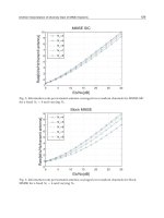
The most popular numerical technique that can b e used for the
solution of the above optimization problem is known as the golden section
search technique. It successively divides the available search range, specified
as [a
i
, b
i
] at every iteration, into two sections proportioned approximately as
(0.319 and 0.681) and discards the one that does not contain the minimum.
The number 0.681 has been discovered as the most efficient way for internal
division by numerous mathematicians (whose derivation can be found in

optimization books, such as the one by J. Kowalik and M. R. Osborne). The
golden section search starts by choosing two x values, x
1
0
and x
2
0
, which
divide the interval [a
0
, b
0
] into three thirds (Fig. 10), and proceeds to the
evaluation of the function at these points, Z(x
1
0
) and Z(x
2
0
) (for example,
through FEA), respectively.
The golden section iterative process compares the two function values,
evaluated at x
1
i
and x
2
i
in Step i, and narrows the search domain accordingly:
(1) If Z(x

1
i
)>Z(x
2
i
)
a
iþ1
¼ x
i
1
; b
iþ1
¼ b
i
x
iþ1
1
¼ x
i
2
and x
iþ1
2
¼ b
iþ1
À 0:319ðb
iþ1
À a
iþ1

Þð5:27Þ
(2) If Z(x
2
i
)>Z(x
1
i
)
a
iþ1
¼ a
i
; b
iþ1
¼ x
i
2
FIGURE 10 Golden section search—an example. First iteration.
Computer-Aided Engineering Analysis and Prototyping 149
Copyright © 2003 by Marcel Dekker, Inc. All Rights Reserved.