Materials Selection and Design (2010) Part 15 docx

unique parts, the domains of cost estimation expand dramatically. So, although domain limitation is necessary for cost-
estimates accuracy, it is not a panacea.
Database Commonality. Estimating the costs of a complex product through various phases of development and
production requires organization of large amounts of data. If the data for design, manufacturing, and cost are linked, there
is database commonality. It has been found (Ref 3) that having database commonality results in dramatic reductions in
cost and schedule overruns in military programs. In the same study, domain limitation was found to be essential in
achieving database commonality.
Having database commonality with domain limitation implies that the links between the design and specific
manufacturing processes, with their associated costs, are understood and delineated. Focusing on specific manufacturing
processes allows one to collect and organize data on where and how costs arise in specific processes. With this focus, the
accuracy of cost estimates can be determined, provided that uniform methods of estimation are used, and provided that,
over time, the cost estimates are compared with the actual costs as they arise in production. In this manner, the accuracy
of complex cost estimates may be established and improved.
In present engineering and design practice, many organizations do not have adequate database commonality, and the
accuracy of cost estimates is not well known. Database commonality requires an enterprise-wide description of cost-
dominant manufacturing processes, a way of tracking actual costs for each part, and a way of giving this information in
an appropriate format to designers and cost estimators. Most "empirical methods" of cost estimation, which are based on
industrywide studies of statistical correlation of cost, may or may not apply to the experience of a specific firm (see the
discussion in the sections that follow).
Costs are "rolled up" for a product when all elements of the cost of a product are accounted for. Criteria for cost
estimation using database commonality is simple: speed (how long does it take to roll up a cost estimate on a new design),
accuracy (what is the standard deviation of the estimate, based on comparison with actual costs) and risk (what is the
probability distribution of the cost estimate; what fraction of the time will the estimate be more than 30% too low, for
example). One excellent indicator of database commonality is the roll-up time criteria. World-class cost-estimation roll-
up times are minutes to fractions of days. Organizations that have such rapid roll-up times have significantly less cost and
schedule overruns on military projects (Ref 3).
Cost allocation is another general issue. Cost allocation refers to the process by which the components of a design are
assigned target costs. The need for cost allocation is clear: how else would an engineer, working on a large project, know
how much the part being designed should cost? And, if the cost is unknown and the target cost is not met, there will be
time delays, and hence costs incurred due to unnecessary design iteration. It is generally recognized that having integrated
product teams (IPTs) is a good industrial practice. Integrated product teams should allocate costs at the earliest stages of a

development program. Cost estimates should be performed concurrently with the design effort throughout the
development process. Clearly, estimating costs at early stages in a development program, for example, when the concept
of the product is being assessed, requires quite different tools than when most or all the details of the design are specified.
Various tools that can be used to estimate cost at different stages of the development process are described later in this
section.
Elements of Cost. There are many elements of cost. The simplest to understand is the cost of material. For example, if
a part is made of aluminum and is fabricated from 10 lb of the material, if the grade of aluminum costs $2/lb, the material
cost is $20. The estimate gets only a bit more complex if, as in the case of some aerospace components, some 90% of the
materials will be machined away; then the sale on scrap material is deducted from the material cost.
Tooling and fixtures are the next easiest items to understand. If tools are used for only one product, and the lifetime of the
tool is known or can be estimated, then only the design and fabrication cost of the tool is needed. Estimates of the
fabrication costs for tooling are of the same form as those for the fabricated parts. The design cost estimate raises a
difficult and general problem: cost capture (Ref 4). For example, tooling design costs are often classified as overhead,
even though the cost of tools relates to design features. In many accounting systems, manufacturing costs are assigned
"standard values," and variances from the standard values are tabulated. This accounting methodology does not, in
general, allow the cost engineer to determine the actual costs of various design features of a part. In the ledger entries of
many accounting systems, there is no allocation of costs to specific activities or no activity-based accounting (ABC) (Ref
5). In such cases there are no data to support design cost estimates.
Direct labor for products or parts that have a high yield in manufacturing normally have straightforward cost estimates,
based on statistical correlation to direct labor for past parts of a similar kind. However, for parts that have a large amount
of rework the consideration is more complex, and the issues of cost capture and the lack of ABC arise again. Rework may
be an indication of uncontrolled variation of the manufacturing process. The problem is that rework and its supervision
may be classified all, or in part, as manufacturing overhead. For these reasons, the true cost of rework may not be well
known, and so the data to support cost estimates for rework may be lacking.
The cost estimates of those parts of overheads that are associated with the design and production of a product are
particularly difficult to estimate, due to the lack of ABC and the problem of cost capture. For products built in large
volumes, of simple or moderate complexity, cost estimates of overheads are commonly done in the simplest possible way:
the duration of the project and the level of effort are used to estimate the overhead. This practice does not lead to major
errors because the overhead is a small fraction of the unit cost of the product.
For highly engineered, complex products built in low volume, cost estimation is very difficult. In such cases the problem

of cost capture is also very serious (Ref 4).
Machining costs are normally related to the machine time required and a capital asset model for the machine, including
depreciation, training, and maintenance. With a capital asset model, the focus of the cost estimate is the time to
manufacture. A similar discussion holds for assembly costs: with a suitable capital asset model, the focus of the cost
estimate is the time to assemble the product (Ref 1).
Methods of Cost Estimations. There are three methods of cost estimation discussed in the following sections of this
article. The first is parametric cost estimation. Starting from the simplest description of the product, an estimate of its
overall cost is developed. One might think that such estimates would be hopelessly inaccurate because so little is specified
about the product, but this is not the case. The key to this method is a careful limitation of the domain of the estimate (see
the previous section). This example deals with the estimate of the weight of an aircraft. The cost of the aircraft would then
be calculated using dollars/pound typical of the aircraft type. Parametric cost estimation is the generally accepted method
of cost estimation in the concept assessment phases of a development program. The accuracy is surprisingly good about
30% (provided that recent product-design evolution has not been extensive).
The second method of cost estimation is empirically based: one identifies specific design features and then uses statistical
correlation of costs of past designs to estimate the cost of the new design. This empirical method is by far the most
common in use. For the empirical method to work well, the features of the product for which the estimate is made should
be unambiguously related to features of prior designs, and the costs of prior designs unambiguously related to design
features. Common practice is to account for only the major features of a design and to ignore details. Empirical methods
are very useful in generating a rough ranking of the costs of different designs and are commonly used for that purpose
(Ref 1, 6, 7). However, there are deficiencies inherent in the empirical methods commonly used.
The mapping of design features to manufacturing processes to costs is not one-to-one. Rather, the same design feature
may be made in many different ways. This difficulty, the feature mapping problem, discussed in Ref 4, limits the
accuracy of empirical methods and makes the assessment of risk very difficult. The problem is implicit in all empirical
methods. The problem is that the data upon which the cost correlation is based may assume the use of manufacturing
methods to generate the features of the design that do not apply to the new design. It is extraordinarily difficult to
determine the implicit assumptions made about manufacturing processes used in a prior empirical correlation. A
commonly stated accuracy goal of empirical cost estimates is 15 to 25%, but there is very little data published on the
actual accuracy of the cost estimate when it is applied to new data.
The final method discussed in this article is based on the recent development called complexity theory. A mathematically
rigorous definition of complexity in design has been formulated (Ref 8). In brief, complexity theory offers some

improvement over traditional empirical methods: there is a rational way to assess the risk in a design, and there are ways
of making the feature mapping explicit rather than implicit. Perhaps the most significant improvement is the capability to
capture the cost impact of essentially all the design detail in a cost estimate. This allows designers and cost estimators to
explore, in a new way, methods to achieve cost savings in complex parts and assemblies.

References cited in this section
1.

G. Boothroyd, P. Dewhurst, and W. Knight, Product Design for Manufacture and Assembly,
Marcel Dekker,
1994, Chapt. 1
3.

D.P. Hoult and C.L. Meador, "Cost Awareness in Design: the Role of Database Commonality," SAE 96008,
Society of Automotive Engineers, 1996
4.

D.P. Hoult and C.L. Meador, "Methods of Integra
ting Design and Cost Information to Achieve Enhanced
Manufacturing Cost/Performance Trade-
Offs," Save International Conference Proceedings, Society for
American Value Engineers, 1996, p 95-99
5.

H.T. Johnson and R.S. Kaplan, Relevance Lost, the Rise and Fall of Management Accounting,
Harvard
Business School Press, 1991
6.

G. Boothroyd, Assembly Automation and Product Design, Marcel Dekker, 1992

7.

P.F. Ostwald, "American Machinist Cost Estimator," Penton Educational Division, Penton Publishing, 1988
8.

D.P. Hoult and C.L. Meador, "Predicting Product Manufacturing Costs from Design Attributes: A
Complexity Theory Approach," No. 960003, Society of Automotive Engineers, 1996
Manufacturing Cost Estimating
David P. Hoult and C. Lawrence Meador, Massachusetts Institute of Technology

Parametric Methods
An example for illustrating parametric cost estimation is that of aircraft. In Ref 9, Roskam a widely recognized
researcher in this field describes a method to determine the size (weight) of an aircraft. Such a calculation is typical of
parametric methods. To determine cost from weight, one would typically correlate costs (inflation adjusted) of past
aircraft of similar complexity with their weight. Thus weight is surrogate for cost for a given level of complexity.
Most parametric methods are based on such surrogates. For another simple example, consider that large coal-fired power
plants, based on a steam cycle, cost about $1500/kW to be built. So, if the year the plant is to be built (for inflation
adjustment) and its kW output is known, parametric cost estimate can be readily obtained.
Parametric cost estimates have the advantage that little needs to be known about the product to produce the estimate.
Thus, parametric methods are often the only ones available in the initial (concept assessment) stages of product
development.
The first step in a parametric cost estimation is to limit the domain of application. Roskam correlates statistical data for a
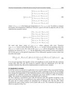
dozen types of aircraft and fifteen sub types. The example he uses to explain the method is that of a twin-engine,
propeller-driven airplane. The mission profile of this machine is given in Fig. 1 (Ref 9).

Fig. 1 Mission profile
Inspection of the mission specifications and Fig. 1 shows that only a modest amount of information about the airplane is
given. In particular, nothing is specified about the detailed design of the machine! The task is to estimate the total weight,
W
TO

or the empty weight, W
E
, of the airplane. Roskam argues that the total weight is equal to the sum of the empty
weight, fuel weight, W
F
, payload and crew weight, W
PL
+ W
crew
, and the trapped fuel and oil, which is modeled as a
fraction, M
tfo
, to the total weight. M
tfo
is to be a small (constant) number, typically 0.001 to 0.005. Thus the fundamental
equation for aircraft weight is:
W
TO
= W
E
+ W
F
+ W
PL
+ W
crew
+ M
tfo
W
TO

(Eq 1)
The basic idea of Roskam is that there is an empirical relationship between aircraft empty and total weights, which he
finds to be:
log
10
W
E
= {(log
10
W
TO
) - A}/B


(Eq 2)
The coefficients, A and B, depend on which of the dozen types and fifteen subtypes of aircraft fit the description in Table
1 and Fig. 1. It is at this point that the principle of domain limitation first enters. For the example used by Roskam, the
correlation used to determine A = 0.0966 and B = 1.0298 for the twin-engine, propeller-driven aircraft spans a range of
empty weights from 1000 to 7000 lb.
Table 1 Mission specification for a twin-engine, propeller-driven airplane
1. Payload Six passengers at 175 lb each (including the pilot) and 200 lb total baggage

2. Range
1000 statute miles with maximum payload
3. Reserves
25% of mission fuel
4. Cruise speed
250 knots at 75% power at 10,000 ft and at takeoff weight

5. Climb
10 min to 10,000 ft at takeoff weight
6. Takeoff and landing

1500 ft ground fun at sea level, standard day. Landing at 0.95 of takeoff weight

7. Powerplants
Piston/propeller
8. Certification base
FAR23

The method proceeds as follows to determine the weight of fuel required in the following way. The mission fuel, W
F
, can
be broken down into the weight of the fuel used and the reserve fuel:
W
F
= W
Fres
+ W
Fused


(Eq 3)
Roskam models the reserve fuel as a fraction of the fuel used (see Table 1). The fuel used is modeled as a fraction of the
total weight, and depends on the phase of the mission, as described in Fig. 1. For mission phases that are not fuel
intensive, a fixed ratio of the weight at the end of the phase to that at the beginning of the phase is given. Again, these
ratios are specific to the type of aircraft. For fuel-intensive phases, in this example the cruise phase, there is a relationship
between the lift/drag ratio of the aircraft, the engine fuel efficiency, and the propeller efficiency. Again, these three
parameters are specific to the type of aircraft.

When the fuel fraction of the total weight is determined by either a cruise calculation, or by the ratio of weight at the end
of a mission phase to the beginning of a mission phase, the empty weight can be written in terms of the total weight. Then
Eq 2 is used to find the total weight of the aircraft.
For the problem posed, Roskam obtains an estimated total weight of 7900 lb. The accuracy can be estimated from the
scatter in the correlation used to determine the coefficients A and B, and is about 30%. For details of the method Roskam
uses for obtaining the solution, refer to Ref 9.
Some limitations of the parametric estimating method are of general interest. For example, if the proposed aircraft does
not fit any of the domains of the estimating model, the approach is of little use. Such an example might be the V-22, a tilt
wing aircraft (Ref 10), which flies like a fixed-wing machine, but tilts its wings and propellers, allowing the craft to hover
like a helicopter during take-off and landing. Such a machine might be considered outside the domain of Roskam's
estimating model. The point is not that the model is inadequate (the V-22 is more recent than Roskam's 1986 article), but
the limited product knowledge in the early stages of development makes it difficult to determine if a cost estimate for the
V-22 fits in a well-established domain.
Conversely, even complex machines, such as aircraft, are amenable to parametric cost estimates with fairly good
accuracy, provided they are within the domain of the cost model. In the same article, Roskam presents data for transport
jets, such as those used by airlines. It should be emphasized that the weight (and hence cost) of such machines, with more
than one million unique parts, can be roughly estimated by parametric methods.
Of course, cost is not the same as weight or, for that matter, any other engineering parameter. The details of the
manufacturing process, inventory control, design change management, and so forth, all play a role in the relationship
between weight and cost. The more complex the machine, the more difficult it is to understand if the domain of the
parametric cost-estimating model is the same as that of the product being estimated.

References cited in this section
9. J. Roskam, Rapid Sizing Method for Airplanes, J. Aircraft, Vol 23 (No.7), July 1986, p 554-560
10.

The Bell-Boeing V-22 Osprey entered Low Rate Initial Production with the MV-
22 contract signed June 7,
1996, Tiltrotor Times, Vol 1 (No. 5), Aug 1996
Manufacturing Cost Estimating

David P. Hoult and C. Lawrence Meador, Massachusetts Institute of Technology

Empirical Methods of Cost Estimation
Almost all the cost-estimating methods published in the literature are based on correlation of some feature or property of
the part to be manufactured. Two examples are presented. The first is from the book by Boothroyd, Dewhurst, and Knight
(Ref 1), hereafter referred to as BDK. Chapter 9 of this book is devoted to "Design for Sheet Metalworking." The first
part of this chapter is devoted to estimates of the costs of the dies used for sheet metal fabrication. This example was
chosen because the work of these authors is well recognized. (Boothroyd and Dewhurst Inc. sells widely used software
for design for manufacture and design assembly.) In this chapter of the book, the concept of "complexity" of stamped
sheet metal parts arises. The complexity of mechanical parts is discussed in the section "Complexity Theory" in this
article.
Example 1: Cost Estimates for Sheet Metal Parts.
Sheet metal comes in some 15 standard gages, ranging in thickness from 0.38 to 5.08 mm. It is commonly available in
steel, aluminum, copper, and titanium. Typical prices for these materials are 0.80-0.90$/lb for low-carbon steel, $6.00-
$7.00/lb for stainless steel, $3.00/lb for aluminum, $10.00/lb for copper, and $20.00/lb for titanium. It is typically shipped
in large coils or large sheets.
Automobiles and appliances use large amounts of steel sheet metal. Aluminum sheet metal is used in commercial aircraft
manufacture, but in lesser amounts due to the smaller number of units produced.
Sheet metal is fabricated by shearing and forming operations, carried out by dies mounted in presses. Presses have beds,
which range in size from 50 by 30 cm to 210 by 140 cm (20 by 12 in. to 82 by 55 in.). The press force ranges from 200 to
4500 kN (45 to 1000 lbf). The speed ranges from 100 strokes/min to 15 strokes/min in larger sizes.
Dies typically have four components: a basic die set; a punch, held by the die set, which shears or forms the metal; a die
plate through which or on which the punch acts; and a stripper plate, which removes the scrap at the end of the fabrication
process.
BDK estimate the basic die set cost (C
ds
, in U.S. dollars) as basically scaling with usable area (A
u
, in cm
2

):
C
ds
= 120 + 0.36A
u


(Eq 4)
The coefficients (Eq 4) arise from correlating about 50 data points of die set cost with useable area. The tooling elements
(the punch, die plate, and stripper plate) are estimated with a point system as follows: let the complexity of the part to be
fabricated be X
p
. Suppose that the profile has a perimeter P (cm), and that the part has an over width and length of W (cm)
and L (cm) of the smallest dimensions which surround the punch. The complexity of the part is taken to be:
X
p
= (P/L)(P/W)


(Eq 5)
The assessment of how part complexity affects cost arises repeatedly in cost estimating. The subject is discussed at length
in the next section "Complexity Theory" . From the data of BDK, the basic time to manufacture the die set (M, in hours)
can be estimated by the following steps: Define the basic manufacturing points (M
po
) as
M
po
= 30 + 0.56

(Eq 6)
Note that the manufacturing time increases a bit less than linearly with part complexity. This is consistent with the section
"Complexity Theory" . BDK goes on to add two correction factors to M
po
. The first is a correction factor due to plate size
and part complexity, f
LW
. From BDK data it is found:
f
LW
= 1 + 0.0276LW


(Eq 7)
The second correction factor is to account for the die plate thickness. BDK cites Nordquist (Ref 11), who gives a
recommended die thickness, h
d
, as:
h
d
= 9 + 2.5 log
e
(U/U
ms
)Vh
2


(Eq 8)
where U is the ultimate tensile stress of the sheet metal, U

ms
is the ultimate stress of mild steel, a reference value, V, is the
required production volume, and h is the thickness (in mm) of the metal to be stamped. BDK recommends the second
correction factor to be:
f
d
= 0.5 + 0.02h
d
or f
d
= 0.75


(Eq 9)
whichever is greater.
The corrected labor hours, M
p
, are then estimated as:
M
p
= f
d
f
LW
M
po


(Eq 10)
The cost of the die is the sum of the corrected labor hours times the labor rate of the die fabricator plus the basic die set

cost, from Eq 4.
As a typical example of the empirical cost estimating methods, the BDK method takes into account several factors such as
the production volume, the strength of the material (relating to how durable the die needs to be), the die size, and
complexity of the part. These factors clearly influence die cost. However, the specific form of the equations are chosen as
convenient representations of the data at hand. (As, indeed, are Eq 6 and 7, derived by fitting BDK data.)
The die cost risk (i.e., uncertainty of the resulting estimate of die cost) is unknown, because it is not known how the
model equations would change with different manufacturing processes or different die design methods.
It is worth noting carefully that only some features of the design of the part enter the cost estimate: the length and width
of the punch area, the perimeter of the part to be made, the material, and the production volume. Thus, the product and die
designers do not need to be complete in all details to make a cost estimate. Hence, the estimate can be made earlier in the
product-development process. Cost trades between different designs can be made at an early stage in the product-
development cycle with empirical methods.
Example 2: Assembly Estimate for Riveted Parts.
The American Machinist Cost Estimator (Ref 7) is a very widely used tool for empirical cost estimation. It contains data
on 126 different manufacturing processes. A spreadsheet format is used throughout for the cost analysis. One example is
an assembly process. It is proposed to rivet the aluminum frame used on a powerboat. The members of the frame are
made from 16-gage aluminum. The buttonhead rivets, which are sized according to recommendations in Ref 12, are
in. in diameter and conform to ANSI standards. Figure 2 shows the part.

Fig. 2 Powerboat frame assembly
There are 20 rivets in the assembly, five large members of the frame, and five small brackets. Chapter 21 in Ref 7
includes six tables for setup, handling, pressing in the rivets, and riveting. A simple spreadsheet (for the first unit) might
look like Table 2. The pieces are placed in a frame, the rivets are inserted, and riveted. The total cycle time for the first
unit is 18.6 min. There are several points to mention here. First, the thickness of the material and the size of the rivets play
no direct part in this simple calculation. The methods of Ref 7 do not include such details.
Table 2 Spreadsheet example for assembly of frame (Fig. 2)

Source
(a)

Process
description
Table time,

min
Setup,

min
21.2-S
Setup 15
21.2-1
Get 5 frame members from skid

1.05
21.2-1
Get 5 brackets from bench 0.21
21.2-2
Press in hardware (20 rivets) 1.41
21.2-3
Set 20 rivets 0.93
Total cycle time (minutes)
3.60 15

(a)
Tables in Ref 7, Chapter 21

Yet common sense suggests that some of the details must count. For example, if the rivet holes are sized to have a very
small clearance, then the "press-in-hardware" task, where the rivets are placed in the rivet holes, would increase. In a like
manner, if the rivets fit looser in the rivet holes, the cycle time for this task might decrease. The point of this elementary

discussion is that there is some implied tolerance with each of the steps in the assembly process.
In fact, one can deduce the tolerance from the standard specification of the rivets. From Ref 12, in the tolerance on in.
diameter buttonhead rivets is 0.010 in. So the tolerance of the hole would be about the same size.
The second point is that there are 30 parts in this assembly. How the parts are stored and how they are placed in the
riveting jig or fixture determines how fast the process is done. With experience, the process gets faster. There is a well-
understood empirical model for process learning. The observation, often repeated in many different industries, is that
inputs decrease by a fixed percentage each time the number of units produced doubles. So, for example, L
i
is the labor in
minutes of the ith unit produced, and L
0
is the labor of the first unit, then:
L
i
= L
0
i


(Eq 11)
The parameter measures the slope of the learning curve. The learning curve effects were first observed and documented
in the aircraft industry, where a typical rate of improvement might be 20% between doubled quantities. This establishes
an 80% learning function, that is, = 0.80. Because this example is fabricated from aluminum, with rivets typical of
aircraft construction, it is easy to work out that the 32nd unit will require 32.7% of the time (6.1 min) compared to the
first unit (18.6 min).
Learning occurs in any well-managed manual assembly process. With automated assembly, "learning" occurs only when
improvements are made to the robot used. In either case, there is evidence that, over substantial production runs and
considerable periods of time, the improvement is a fixed percentage between doubled quantities. That is, if there is a 20%
improvement between the tenth and twentieth unit, there will likewise be a 20% improvement between the hundredth and
two hundredth unit.

The cost engineer should remember that, according to this rule, the percentage improvement from one unit to the next is a
steeply falling function. After all, at the hundredth unit, it takes another hundred units to achieve the same improvement
as arose between the 10th and 20th units (Ref 13).

References cited in this section
1. G. Boothroyd, P. Dewhurst, and W. Knight, Product Design for Manufacture and Assembly,
Marcel
Dekker, 1994, Chapt. 1
7. P.F. Ostwald, "American Machinist Cost Estimator," Penton Educational Division, Penton Publishing, 1988

11.

W.N. Nordquist, Die Designing and Estimating, 4th ed., Huebner Publishing, 1955
12.

E. Oberg, F.D. Jones, and H.L. Horton, Machinery's Handbook, 22nd ed., Industrial Press, 1987, p 1188-
1205
13.

G.J. Thuesen, and W.J. Fabrycky, Engineering Economy, Prentice Hall, 1989, p 472-474
Manufacturing Cost Estimating
David P. Hoult and C. Lawrence Meador, Massachusetts Institute of Technology

Complexity Theory
Up to now this article has dealt with the cost-estimation tools that do not require a complete description of the part or
assembly to make the desired estimates. What can be said if the design is fully detailed? Of course, one could build a
prototype to get an idea of the costs, and this is often done, particularly if there is little experience with the manufacturing
methods to be used. For example, suppose there is a complex wave feed guide to be fabricated out of aluminum for a
modern radar system. The part has some 600 dimensions. One could get a cost estimate by programming a numerically
controlled milling machine to make the part, but is there a simpler way to get a statistically meaningful estimate of cost,

while incorporating all of the design details? The method that fulfills this task is complexity theory.
There has been a long search for the "best" metric to measure how complex a given part or assembly is. The idea of using
dimensions and tolerances as a metric comes from Wilson (Ref 14). The idea presented here is that the metric is a sum of
log (d
i
/t
i
), where d
i
is the ith dimension and t
i
is its associated tolerance (i ranges over all the dimensions needed to
describe the part). According to complexity theory, how complex a part is, I, is measured by:


(Eq 12)
Originally, the log function was chosen from an imperfect analogy with information theory. It is now understood that the
log function arises from a limit process in which tolerance goes to zero while a given dimension remains fixed. In this
limit, if good engineering practice is followed, that is, if the accuracy of the machine making the part is not greatly
different than the accuracy required of the part, and if the "machine" can be modeled like a first-order damped system,
then it can be shown that the log function is the correct metric. Because of historical reasons, the log is taken to the base
2, and I is measured in bits. Thus Eq 12a is written:


(Eq 12a)
There are two main attractions of the complexity theory. First, I will include all of the dimensions required to describe the
part. Hence, the metric captures all of the information of the original design. For assemblies, the dimensions and
tolerances refer to the placement of each part in the assembly, and second, the capability of making rigorous statements of
how I effects costs. In Ref 8 it is proven that if the part is made by a single manufacturing process, the average time (T) to
fabricate the part is:

T = A · I, A = const


(Eq 13)
Again, in many cases, the coefficient A must be determined empirically from past manufacturing data. The same formula
applies to assemblies made with a single process, such as manual labor. The extension to multiple processes is given in
Ref 8.
A final aspect of complexity theory worth mentioning is risk. Suppose a part with hundreds of dimensions is to be made
on a milling machine. The exact sequence in which each feature of the part is cut out will determine the manufacturing
time. But there are a large number of such sequences, each corresponding to some value of A. Hence there is a collection
of As, which have a mean that corresponds to the average time to fabricate the part. That is the meaning of Eq 13.
It can be shown that the standard deviation of manufacturing time is:
s
T
=
A
I


(Eq 14)
where
T
is the standard deviation of the manufacturing time, and
A
is the standard deviation of the coefficient A.
A

can be determined from past data. These results have a simple interpretation: Parts or assemblies with tighter (smaller)
tolerances take longer to make or assemble because with dimensions fixed, the log functions increase as the tolerances
decrease. More complex parts, larger I, take longer to make (Eq 13), and more complex parts have more cost risk (Eq 14).

These trends are well known to experienced engineers.
In Eq 8, a large number of parts from three types of manufacturing processes were correlated according to Eq 13. The
results of the following manual lathe process are typical of all the processes studied in Eq 8. Figure 3 shows the
correlation of time with I, the dimension information, measured in bits. An interesting fact, shown in Fig. 4 is that the
accuracy of the estimate is no different than that of an experienced estimator.

Fig. 3 Manufacturing time and dimension information for the lathe process (batch size 3 to 6 units)


Fig. 4 Accuracy comparison for the lathe process
In Eq 13, the coefficient, A, is shown to depend on the machine properties such as speed, operation range, and time to
reach steady-state speed. Can one estimate their value from first principals? It turns out that for manual processes one can
make rough estimates of the coefficient.
The idea is based on the basic properties of human performance, known as Fitts' law. Fitts and Posner reported the
maximum human information capacity for discrete, one-dimensional positioning tasks at about 12 bits/s (Ref 15). Other
experiments have reported from 8 to 15 bits/s for assembly tasks (Ref 16).
The rivet insertion process discussed previously in this article is an example. The tolerance of the holes for the rivets is
estimated to be 0.010 in., that is, the same as the handbook value of the tolerance of the barrel of the rivet (Ref 12). Then
it is found that d/t 0.312/0.010 = 31.2 and log
2
= 4.815 bits for each insertion. The initial rate of insertion (Ref 7) was
20 units in 1.41 min. That corresponds to A = 1.14 bits/s. Clearly, there is some considerable improvement available if the
maximum values quoted (Ref 15, 16) can be achieved for rivet insertion.
Example 3: Manual Assembly of a Pneumatic Piston.
In Ref 1 there is an extensive and helpful section on manual assembly. The method BDK used categorizes the difficulty of
assembling parts by a number of parameters, such as the need to use one or two hands, the need to use mechanical tools,
part symmetry, and so on. Figure 5 (reproduced from an example in Ref 17) shows the assembly of a small pneumatic
piston. Table 3 lists assembly times.
Table 3 Assembly times for piston example (Fig. 5)
Part

ID No.

No. times operation

carried out
Handling code

Time, s

Insertion code

Insertion time, s

Total time, s

Pneumatic piston

7
1 30 1.95 00 1.5 3.45 Block
6
1 15 2.25 22 6.5 8.75 Piston
5
1 10 1.50 00 1.5 3.0 Piston stop
4
1 80 4.10 00 1.5 5.6 Spring
3
1 28 3.18 09 7.5 10.7 Cover
2
2 68 8.00 39 8.0 29.0 Screw
Total time: 60.5

Fig. 5 Assembly of pneumatic piston. Dimensions in millimeters

Consider the entries for the two screws. The handling code, 68, describes a part with 360° symmetry that can be handled
with standard tools. The insertion code, 39, describes a part not easy to align or position. The time for assembly of the
screws is nominally 32 s, less an allowance of 31 s for repetitive operations.
Now consider a simplified design (Fig. 6 and Table 4). The same tables from Chapter 21 in Ref 7 are used as in Table 2.
Software is available to automate the table look-up process. For the same problem using complexity theory, there is only
one coefficient, A = 1.5 bits/s for the small manual assembly. This value is found by calculating the bits of information in
the initial design and using the time found in Ref 17 to determine A.
Table 4 Assembly times for simplified piston design (Fig. 6)
Part
ID No.

No. times operation

carried out
Handling code

Time, s

Insertion code

Insertion time, s

Total time, s

Pneumatic

piston
4
1 30 1.95 00 1.5 3.45 Block
3
1 15 2.25 00 1.5 3.75 Piston
2
1 80 4.10 00 1.5 5.6 Spring
1
1 10 1.50 30 2.0 3.5 Cover/stop

Total time: 16.3


Fig. 6 Simplified assembly of pneumatic piston. Dimensions in millimeters

The tolerances were obtained in the following way. For the screws, the size was chosen to be M3X0.5 a coarse thread
metric size consistent with insertion into molded nylon. As reported in Ref 12, the tolerance is ANSI B1.13M-1979.
The spring tolerance is derived using a standard wire size, 0.076 in. (0.193 mm), which gives a spring index D/d = 12.95,
(D = spring diameter, d = wire diameter) well within the Spring Manufacturers Institute recommended range. The
tolerance quoted is the standard tolerance for this wire diameter and spring index.
The plastic parts are presumed to be injection molded, with a typical tolerance of 0.1 mm. The screws are assumed to
tighten to a tolerance of = th of a turn.
These data, which can be easily verified in practice, give essentially the same results as the other empirical methods.
Calculations for the original design (Fig. 5) and the simplified design (Fig. 6) are compared in Tables 5 and 6,
respectively. This compares well with the results of Ref 17 (73% reduction) versus 76% reduction here.
Table 5 Original manual assembly design
Feature (No.)

Dimensions, mm

Tolerance

Bits Notes
2
3 0.063 11.14693

Diameter dimension
2
30 0.1 16.45764

Horizontal location
2
30 0.1 16.45764

Horizontal location
2
2160 60 10.33985

6 turns to install screw
Subtotal
54.40206


1
31 0.1 8.276124

Horizontal location of plate

1
31 0.1 8.276124

Horizontal location of plate

Subtotal
70.95431


1
25 0.43 5.861448

Spring location
Subtotal
76.81575


1
25 0.1 7.965784

Piston location
Subtotal
84.78154


1
25 0.1 7.965784

Piston stop
Total:
92.74732

1.5 bits/s

Table 6 Simplified manual assembly design
Feature

(No.)
Dimensions,

mm
Tolerance

Bits Notes
1
25 0.1 7.965784

Piston location
1
25 0.43 5.861448

Spring location
1
25 0.1 7.965784

Piston cap
Total:
21.79302

% reduction 76.50281

There are two comments to make:
• This method requires only one coefficient for hand assembly of small parts. A 1.6 bits/s and no look-
up tables.
• One can make small changes in design, for example, change the screw size, and get an indication o
f the
change in assembly time.
If one started with a preliminary design, the assembly time estimate would grow more accurate as more details of the
design itself and the manufacturing process to build the design become known. However, the methods of Boothroyd, and
others (Ref 1, 6, 17), require less data than does the complexity theory.
In the simplified manufacturing process, the coefficient A = 1.6 bits/s is substantially less than the Fitts' law (discussed
earlier in this section on complexity theory) value of 8 bits/s. The discrepancy may lie in the time it takes an assembler to
pick up and orient each part before the part is assembled. Jigs and trays, and so forth, that reduce this pick-and-place
orientation effort would save assembly time. As before, there is some considerable improvement available if the
maximum values quoted (Ref 15, 16) can be achieved for manual assembly. The value obtained here (A = 1.16) is close to
that deduced from Ref 7 for the hand insertion of rivets.
Using complexity theory and a single assembly process, the ratio of the assembly times can be calculated with out any
knowledge of the coefficient, A. Thus complexity theory offers advantages when a single process is used, even if little or
nothing is known about the performance of the process.

References cited in this section
1. G. Boothroyd, P. Dewhurst, and W. Knight, Product Design for Manufacture and Assembly,
Marcel
Dekker, 1994, Chapt. 1
6. G. Boothroyd, Assembly Automation and Product Design, Marcel Dekker, 1992
7. P.F. Ostwald, "American Machinist Cost Estimator," Penton Educational Division, Penton Publishing, 1988

8. D.P. Hoult and C.L. Meador, "Predicting Product Manufacturing Costs from Design Attributes
: A
Complexity Theory Approach," No. 960003, Society of Automotive Engineers, 1996
12.

E. Oberg, F.D. Jones, and H.L. Horton, Machinery's Handbook, 22nd ed., Industrial Press, 1987, p 1188-
1205
14.

D.R. Wilson, "An Exploratory Study of Complexity in Axio
matic Design," Doctoral Thesis, Massachusetts
Institute of Technology, 1980
15.

P.M. Fitts, and M.I. Posner, Human Performance, Brooks/Cole Publishing, Basic Concepts in Psychology
Series, 1967
16.

J. Annett, C.W. Golby, and H. Kay, The Measurement of Elements in an Assembly Task
The Information
Output of the Human Motor System, Quart. J. Experimental Psychology, Vol 10, 1958
17.

G. Boothroyd and P. Dewhurst, Product Design for Assembly, Boothroyd Dewhurst, 1989
Manufacturing Cost Estimating
David P. Hoult and C. Lawrence Meador, Massachusetts Institute of Technology

Cost Estimation Recommendations
Which type of cost estimate one uses depends on how much is know about the design. In the early stages of concept
assessment of a new part or product, parametric methods, based upon past experience, are preferred. Risk is hard to
quantify for these methods, because it can be very difficult to determine whether the new product really is similar to those
used to establish the parametric cost model.
If there is some detailed information about the part or product, and the method of manufacturing is well known, then the
empirical methods should be used. They can indicate the relative cost between different designs and give estimates of

actual costs.
If detailed designs are specified, and a single manufacturing process is to be used, complexity theory should be used to
compare the relative costs and cost risks of the different designs, even if the manufacturing process is poorly understood.
If there are detailed designs available, and well-known manufacturing methods are used, either complexity theory or
empirical methods can be used to generate cost estimates. If a rigorous risk assessment is needed, complexity theory
should be used.




Manufacturing Cost Estimating
David P. Hoult and C. Lawrence Meador, Massachusetts Institute of Technology

References
1. G. Boothroyd, P. Dewhurst, and W. Knight, Product Design for Manufacture and Assembly,
Marcel
Dekker, 1994, Chapt. 1
2. K.T. Ulrich and S.A. Pearson, "Does Produc
t Design Really Determine 80% of Manufacturing Cost?,"
working paper 3601-93-MSA, MIT Sloan School, Nov 1994
3.
D.P. Hoult and C.L. Meador, "Cost Awareness in Design: the Role of Database Commonality," SAE 96008,
Society of Automotive Engineers, 1996
4.
D.P. Hoult and C.L. Meador, "Methods of Integrating Design and Cost Information to Achieve Enhanced
Manufacturing Cost/Performance Trade-
Offs," Save International Conference Proceedings, Society for
American Value Engineers, 1996, p 95-99
5. H.T. Johnson and R.S. Kaplan, Relevance Lost, the Rise and Fall of Management Accounting,
Harvard

Business School Press, 1991
6. G. Boothroyd, Assembly Automation and Product Design, Marcel Dekker, 1992
7. P.F. Ostwald, "American Machinist Cost Estimator," Penton Educational Division, Penton Publishing, 1988

8.
D.P. Hoult and C.L. Meador, "Predicting Product Manufacturing Costs from Design Attributes: A
Complexity Theory Approach," No. 960003, Society of Automotive Engineers, 1996
9. J. Roskam, Rapid Sizing Method for Airplanes, J. Aircraft, Vol 23 (No.7), July 1986, p 554-560
10.

The Bell-Boeing V-22 Osprey entered Low Rate Initial Production with the MV-
22 contract signed June 7,
1996, Tiltrotor Times, Vol 1 (No. 5), Aug 1996
11.

W.N. Nordquist, Die Designing and Estimating, 4th ed., Huebner Publishing, 1955
12.

E. Oberg, F.D. Jones, and H.L. Horton, Machinery's Handbook, 22nd ed., Industrial Press, 1987, p 1188-
1205
13.

G.J. Thuesen, and W.J. Fabrycky, Engineering Economy, Prentice Hall, 1989, p 472-474
14.

D.
R. Wilson, "An Exploratory Study of Complexity in Axiomatic Design," Doctoral Thesis, Massachusetts
Institute of Technology, 1980
15.

P.M. Fitts, and M.I. Posner, Human Performance, Brooks/Cole Publishing, Basic Concepts in Psychology
Series, 1967
16.

J. Annett, C.W. Golby, and H. Kay, The Measurement of Elements in an Assembly Task
The Information
Output of the Human Motor System, Quart. J. Experimental Psychology, Vol 10, 1958
17.

G. Boothroyd and P. Dewhurst, Product Design for Assembly, Boothroyd Dewhurst, 1989
Design for Casting
Thomas S. Piwonka, The University of Alabama

Introduction
CASTING offers the designer cost advantages over other manufacturing methods for most components, especially those
having complex geometries. Casting properties are usually isotropic, and castings may be designed for function rather
than for ease of assembly, like built-up structures. Fillet radii are usually generous, decreasing stress concentration
factors. Converting a built-up assembly to a casting is usually accompanied by a decrease in part count, assembly time,
and inventory, and a savings in weight. With the development of rapid prototyping, expensive tooling is not necessary,
and parts can be delivered within days after the order is placed. The casting process is well understood, and high integrity
castings are as reliable as forgings. Indeed, castings prove their quality everyday in applications as demanding as
prostheses, automotive chassis components, primary aircraft structures, and rotating hardware in gas turbine engines.
Designers face a number of challenges in the design of castings. To begin with, there are a wide variety of casting alloys.
Complete mechanical property data, especially for dynamic properties, are sometimes lacking for these alloys. Static
property data, though often found in handbooks, may consist of "typical values," which are of little help in creating an
efficient design. These typical values obscure a crucial fact: casting properties are determined during solidification and
subsequent heat treatment. This means that properties will vary depending on how quickly the casting solidifies and how
the casting is heat treated.
Thus, to create effective designs, designers should be acquainted with fundamental information about how casting design
influences casting solidification and how casting solidification influences casting properties. This article approaches

design by reviewing the aspects of castings with which designers should be familiar. It also reviews methods used by
foundries to produce high-integrity castings. Specification of casting quality levels should be based on solid knowledge of
the effect of casting discontinuities and on component testing. Procurement of high-quality castings requires the
involvement of the designer, the purchasing agent, and the foundry in a cooperative effort.
Design for Casting
Thomas S. Piwonka, The University of Alabama

Design Considerations
Casting design begins with the determination of the stresses that must be supported by the cast component and the
geometrical constraints on that component. The designer then arranges the cast material to support the stresses in the most
efficient way. However, in designing a part that will be cast, the designer will optimize the design by taking into account
characteristics of the casting process. Because the properties of the casting determine its performance, those features of
the casting process that affect the casting properties are reviewed here. This discussion emphasizes those concepts that
designers and foundries can use to obtain maximum performance from cast parts.
Designers must begin the design process with a thorough understanding of what properties the component must have in
addition to strength and ductility. Fundamental properties such as Young's modulus, Poisson's ratio, density, thermal
conductivity, and coefficient of thermal expansion vary between alloy families and within alloy families. Cast alloy
selection should begin by taking these differences into account.
How the Casting Process Affects Casting Properties. The properties of a component depend on the way it is
made because the microstructure of the component depends on the manufacturing method, and the properties depend in
turn on the microstructure. Thus the choice of making a part by casting, by forging, or by machining will affect the
performance of the part. Once the decision is made on how the part is to be manufactured, the details of the processing
parameters employed also affect component properties.
Component design is usually approached with the assumption that the material is uniform and isotropic and that there is
an inherent small and random scatter in properties. Exceptions are made for fiber-reinforced composite materials and for
components where directionality of properties is beneficial (directionally solidified gas turbine blades, for example). In
castings, properties will be uniform in specific casting sections from casting to casting provided that the casting variables
are constant for each casting. However, they may vary in a predictable manner from point to point within the casting.
Casting microstructure is determined by cooling rate, that is, how fast each part of the casting freezes. The cooling rate is
roughly proportional to the ratio of the square of the surface area of the casting to the square of its volume (a consequence

of what metal casters know as Chvorinov's law). In other words, bulky castings freeze much slower than thin castings a
sphere of a given volume will freeze more slowly than a thin plate of the same volume because the plate has much more
surface area to transfer the same quantity of heat into the mold. Because the sphere solidifies more slowly, its
microstructure will be coarser than that of the plate even if both are poured from the same melt at the same temperature.
Because microstructure determines casting properties, the properties of the sphere and the plate will be different.
Casting is the solidification of liquid confined in a mold, which shapes the final component. A cavity is made in a mold,
which may be a reusable aggregate, such as sand, or a metal mold, used in permanent mold and die casting. The metal is
delivered to the mold cavity through channels in the mold or die, which are called runners. The passages between the
runner and the mold cavity, where the metal enters the mold, are called gates.
Castings are frequently complex shapes made up of some bulky sections and some thin sections. Obviously, the thin
sections will solidify faster than the thick sections; therefore, their properties will differ from those of the thick sections.
Certain other geometric features will also influence solidification rate. For instance, concave sections, or reentrant angles,
solidify more slowly than fins or protrusions, again affecting the resultant local structure and the properties. In other
words, property variation within a casting, which is caused by local differences in cooling rate, is natural, expected, and
entirely reproducible it is not "random" scatter. It can be predicted and should be taken into account during component
design to enhance the component performance.
One way to take account of this during the design phase is to apply a "section size" effect, a factor by which the local
casting properties are adjusted based on local dimensions. While this technique is often effective, the designer should
remember that casting properties depend on cooling rate, not section size. Cooling rate depends not only on section size
but also on pouring temperature, mold material, gating system, the presence or absence of chills in the mold, mold
coatings, and insulation. Thus, within limits (some very broad), the properties can be controlled by the metal caster to
produce those which the designer desires.
Cast iron provides the most dramatic example of the differences in properties caused by differences in structure resulting
from cooling rate differences. When cast iron (which is essentially a solution of carbon and silicon in iron) solidifies, the
carbon can take different forms, depending on its composition and solidification rate and the way the metal has been
treated during melting. Chill cast iron (white iron) has properties completely different from gray iron of the same
composition, caused solely by the accelerated cooling rate in the "chilled" iron. White iron freezes so quickly that the
carbon combines with the iron to solidify as the compound Fe
3
C, known as cementite because it is hard and brittle. In

gray iron, which solidifies more slowly, the carbon appears as graphite flakes; this iron is easy to machine.
Ductile iron also has properties significantly different from gray iron; in this case the carbon solidifies as tiny spheres in a
steel matrix. Since the spheres of graphite are less effective as stress raisers, compared to the flakes of carbon in gray iron,
ductile iron has significant ductility, whereas gray iron does not, even though they both may have nearly identical
compositions. In this case, the difference in structure, which produces the property difference, is caused not by cooling
rate, but by chemical treatment of the melt, which alters the undercooling at the beginning of solidification, which in turn
affects the way the carbon solidifies. It is important here to realize that in castings, similar compositions, in similar
geometries, can have very different properties, depending on the way the castings are made.
Designers frequently use handbook data in designing components. Very often, these data are developed using Gaussian
statistics. As noted above, such data can be misleading if not corrected to reflect differences in cooling rate from section
to section within a casting. Gaussian statistics are appropriate for those materials that are truly ductile, meaning those that
have a tensile elongation over 8 to 10%. Many casting alloys, however, when completely free of discontinuities, have
elongations of only 5 to 10%. Indeed, this is often the reason that these alloys are commonly cast: their low ductilities
make them hard to form by forging or machining. Use of Gaussian statistics to determine design allowables in these
alloys is incorrect, leads to "casting factors," and causes significant overdesign, waste of material, and weight penalties.
Casting factors are arbitrary increases in casting section thickness applied to compensate for perceived lack of
reproducibility of casting properties. Such factors are unnecessary and wasteful (Ref 1). For this reason, it is important
that designers recognize that designing with low ductility (not brittle) materials requires a different approach than
designing with ductile materials. Also, casting versions of wrought alloys may have different compositions than the
wrought alloys to aid in solidification.
Reproducibility of properties produced by a process is most important for the designer because the components that
are designed must behave according to the design. Reliability is often evaluated using Weibull statistics (Ref 2), which
consider the probability of the existence of a discontinuity that would cause failure. This is particularly appropriate for the
design of low ductility materials. In analyzing data using Weibull statistics, one evaluates the value of the Weibull
modulus. The higher the Weibull modulus is, the more reliable the material will be (that is, the higher the Weibull
modulus, the less the variation in property within a given section of the component).
For tensile properties, ceramics typically have Weibull moduli of approximately 10. Aluminum alloy forgings typically
have Weibull moduli of approximately 50. Conventionally cast aluminum castings have Weibull moduli of approximately
30; using techniques for "premium quality castings," castings with Weibull moduli of 50 are routinely produced for use as
primary structures for commercial aircraft (Ref 3, 4). For carefully made thin sections, the Weibull modulus can be above

80 (Ref 5), well above that expected for forgings.
Ductile iron, most cast steel alloys, and copper-base alloys commonly have high ductilities, and the use of Gaussian
statistics to determine design allowables is appropriate. However, gray and compacted graphite iron, superalloys, some
tool steels, and many aluminum alloys are low ductility alloys and should be approached using Weibull statistics.
Basic Features of Solidification. Solid and liquid alloys usually have different densities, which means when
solidification is complete, the solid will occupy less space than the liquid (in most alloys). In other words, the solid
"shrinks." Because solid metal is more dense than liquid metal, the metal shrinks when it solidifies, and the final casting
will not fill the mold unless this shrinkage is compensated. To do this, the foundry adds a riser to the casting. This riser is
a reservoir of molten metal, which supplies liquid metal to the solidifying casting and compensates for the shrinkage that
occurs. If the riser is to function properly, the liquid metal that it contains must be able to flow through the solidifying
casting to reach the areas in the casting where solidification and hence shrinkage is occurring.
In alloy solidification, the picture is complicated by the fact that alloys freeze over a range of temperatures. This means
that small nuclei of solid grains form at the beginning of solidification and grow (forming dendrites, the term for
solidifying grains) as the temperature in the casting falls and solidification progresses. As these grains grow, they form a
"mush" of liquid and solid, which becomes progressively more solid until solidification is complete. Because each small
dendrite that forms is a site where shrinkage occurs during solidification, feeding the shrinkage means finding a way to
cause metal to flow between the dendrites to the location where solidification (and shrinkage) is taking place. As the
dendrites grow, the paths that deliver liquid metal from the riser to the areas where solidification is taking place become
smaller until they are at last too narrow to allow metal to pass. (There is one exception to this rule. In cast iron, both gray
and ductile, the graphite that solidifies expands on solidification. Because graphite forms at the end of solidification, its
expansion often (but not always) compensates for the shrinkage of the iron. For this reason, cast iron often needs very
little in the way of risers.)
Liquid metal can dissolve much more gas in solution than solid metal. Therefore, when metal solidifies, gas that is present
in the liquid is rejected and forms bubbles. A commonly encountered example is that of hydrogen in aluminum. If these
bubbles are trapped in the casting when it freezes, the result is a pore. Pores that result from gas may be spherical,
indicating that they formed early in solidification when the metal was mostly liquid, or they may be interdendritic in
shape, showing that they formed late in solidification, when the liquid that remained was present between dendrites.
As the solidification rate increases, the microstructure of the casting is refined. That is, the grains are smaller, and the
spacing between the arms of the dendrites that make up grains is finer. Mechanical properties usually improve as the
microstructure becomes finer. Because the properties depend on the microstructure, which depends on the solidification

rate, which in turn depends on the processing variables used by the foundry and the casting design, designers have a
major influence on the final properties of the casting.
Using solidification simulation programs, foundries predict how fast each section of each casting will solidify and,
therefore, what will be the properties of each section. The use of these programs combined with the application of
statistical process control techniques has transformed casting into a high technology manufacturing process capable of
reliably producing critical components for the most demanding applications.
General Design Considerations for Castings. Casting design influences the way the casting solidifies because the
geometry of the casting influences how fast each section solidifies; therefore, it is a major factor in determining how
castings will perform. The overarching principle of good casting design is that casting sections should freeze
progressively, allowing the risers to supply liquid metal to feed shrinkage that occurs during solidification. There are a
number of excellent summaries of principles of good casting design (Ref 6, 7, 8), and a comprehensive booklet was
published on design of premium quality aluminum alloy castings (Ref 9). This latter publication also includes general
information on the specification and process of approving foundry sources, which is applicable to castings made from any
metal.
Designing for progressive solidification requires tapering walls so that they freeze from one end to the other, as shown in
Fig. 1, and avoiding situations where two heavy sections are separated by a thin section. (This is a poor design because
metal must feed one heavy section through the thin section; when the thin section freezes before the heavy section, the
flow path will be cut off and shrinkage may form in the heavy section.)

Fig. 1 Redesign of castings to provide progressive solidification through the use of tapered walls.
(a) Elbow
design. (b) Valve fitting design. Source: Ref 10
Junctions also concentrate heat, leading to areas in the casting where heat is retained. These areas solidify more slowly
than others, thus having a coarser structure and different properties from other sections, and solidify after the rest of the
casting has solidified, so that shrinkage cannot be fed. Minimizing the concentration of heat in junctions, therefore, aids in
improving casting properties. Examples of this are shown in Fig. 2.

Fig. 2 Redesign of a casting to minimize heat concentration. (a) Design has n
umerous hot spots (X junctions)
that will cause the casting to distort. (b) Improved design using Y junctions. Source: Ref 6

Concave corners concentrate heat, so they freeze later and more slowly than straight sections, while convex corners lose
heat faster, and freeze sooner and more quickly than straight sections. In designing a casting, the designer should use
properties from test bars that have solidified at the actual cooling rate in that section of the casting. This cooling rate can
be determined by instrumenting a casting and measuring the cooling rate in various sections or by simulating its
solidification using a commercial solidification simulation program.
The hollow spaces in castings are formed by cores, refractory shapes placed in the molds and around which the casting
freezes. These cores are later removed from the casting, usually by thermal or mechanical means. However, each core
requires tooling to form it and time to place it in the mold. Casting designs that minimize cores are preferable to minimize
costs. Some examples are given in Fig. 3.

Fig. 3 Redesign of castings to eliminate cores. (a) C
asting redesigned to eliminate outside cores. (b)
Simplification of a base plate design to eliminate a core. (c) Redesign of a bracket to eliminate a core and to
decrease stress problems. Source: Ref 10
The designer must provide surfaces for the attachment of gates and risers. The casting must solidify toward the riser in
order to be sound, and gates must be located so that the mold fills from the bottom to the top so that oxide films that form
are swept to the top surface of the casting or into risers where they will not affect casting properties. Gate and riser
locations must be accessible for easy removal to minimize processing costs. The position of gate and riser contacts may
also add costs if they are placed where subsequent machining will be required to remove gate stubs or riser pads in the
finished component.

References cited in this section
1. J. Gruner, "Struct
ural Aluminum Aircraft Casting with No Casting Factor," presented at Aeromat '96
(Dayton, OH), ASM International, June 1996
2. W. Weibull, A Statistical Distribution Function of Wide Applicability, J. Appl. Mech., Vol 18, 1951, p 293
3. J. Campbell, J. Runyoro, and S.M.A. Boutorabi, Critical Gate Velocities for Film-Forming Alloys,
AFS
Trans., Vol 100, 1992, p 225
4. N.R. Green and J. Campbell, Proc. Spring 1993 Meeting

(Strasbourg, France), European Division Materials
Research Society, 4-7 May, 1993
5. N.R. Green and J. Campbell, The Influence of Oxide Film Filling Defects on the Strength of Al-7Si-
Mg
Alloy Castings, AFS Trans., Vol 102, 1994, p 341
6. Manufacturing Considerations in Design, Steel Castings Handbook,
5th ed., P.F. Wieser, Ed., Steel
Founders' Society of America, 1980, p 5-6
7. Materials Handbook, Vol 15, Casting, ASM International, 1988, p 598
8. Investment Casting, P.R. Beeley and R.F. Smart, Ed., The Institute of Materials, 1995, p 334
9. Design and Procurement of High-Strength Structural Aluminum Castings,
S.P. Thomas, Ed., American
Foundrymen's Society, 1995
10.

Manufacturing Design Considerations, Chap. 7, Steel Castings Handbook,
6th ed., M. Blair and T.L.
Stevens, Ed., Steel Founders' Society of America and ASM International, 1995
Design for Casting
Thomas S. Piwonka, The University of Alabama

The Effect of Casting Discontinuities on Properties
Poor casting design can interfere with the ability of the foundry to use the best techniques to produce reliable castings.
The designer also specifies the quality requirements that ensure that the cast component will perform as desired. Over
specification causes needless expense and can be avoided by understanding the effect of discontinuities on casting
performance and the effect of casting design on the tendency for discontinuities to form during the casting process.
Important types of casting discontinuities include porosity, inclusions, oxide films, second phases, hot tears, metal
penetration, and surface defects.
Porosity is a common defect in castings and takes many forms. Pores may be connected to the surface, where they can
be detected by dye penetrant techniques, or they may be wholly internal, where they require radiographic techniques to

discover. Macroporosity refers to pores that are large enough to see with the unaided eye on radiographic inspection,
while microporosity refers to pores that are not visible without magnification.
Both macroporosity and microporosity are caused by the combined action of metal shrinkage and gas evolution during
solidification. It has been shown (Ref 11, 12) that nucleation of pores is difficult in the absence of some sort of substrate,
such as a nonmetallic inclusion, a grain refiner, or a second phase particle. This is why numerous investigations have
shown that clean castings, those castings that are free from inclusions, have fewer pores than castings that contain
inclusions. Microporosity is found not only in castings, but also in heavy section forgings that have not been worked
sufficiently to close it up.
When the shrinkage and the gas combine to form macroporosity, properties are deleteriously affected. Static properties
are reduced at least by the portion of the cross-sectional area that is taken up with the pores (since there is no metal in the
pores, there is no metal to support the load there, and the section acts as though its area was reduced). Because the pores
may also cause a stress concentration in the remaining material (Ref 13, 14), static properties may be reduced by more
than the percentage of cross-sectional area that is caused by the macroporosity.
Dynamic properties are also affected. A study of aluminum alloys showed that fatigue properties in some were reduced
11% when specimens having x-ray quality equivalent to ASTM E 155 level 4 were tested, and that they were reduced
17% when specimens having quality of ASTM E 155 level 8 were tested (Ref 15).
Static properties are mostly unaffected by microporosity. Microporosity is found between dendrites and, like
macroporosity, is caused by the inability of feed metal to reach the interdendritic areas of the casting where shrinkage is
occurring and where gas is being evolved. However, because this type of porosity occurs late in solidification, particularly
in long-range freezing (mushy-freezing) alloys, it is particularly difficult to eliminate. The most effective method is to
increase the thermal gradient (often accomplished by increasing the solidification rate), which decreases the length of the
mushy zone. This technique may be limited by alloy and mold thermal properties, and by casting geometry, that is, the
design of the casting.
As long as the micropores are less than 0.2 mm in length, there is no effect on dynamic properties; fatigue properties of
castings with pores that size or smaller are in the same range as those of castings where no micropores were found (Ref
16, 17, 18). The shape of the micropore is as important as its size, with elongated pores having a greater effect than round
pores (Ref 19). Areas where microporosity is expected can be predicted by solidification modeling, similar to the
prediction of macroporosity (see below). Microporosity can be healed by hot isostatic pressing (HIP). In one study
comparing HIP and non-HIP samples, no difference was found in fatigue lives of HIP and non-HIP samples (Ref 20).
However, the HIP samples showed a lower crack growth rate than non-HIP samples. In another study (Ref 21), HIP

improved fatigue crack growth resistance only close to threshold levels. (Additional information about HIP is provided in
the section "Hot Isostatic Pressing" in this article.) As noted above, the design of the casting directly affects its tendency
to solidify in a progressive manner, thereby affecting both the quality and the price of the cast component.
Porosity and casting costs are minimized in casting designs that emphasize progressive solidification toward a gate or
riser, tapered walls, and the avoidance of hot spots.
Inclusions are nonmetallic particles that are found in the casting. They may form during solidification as some elements
(notably manganese and sulfur in steel) precipitate from solution in the liquid. More frequently, they are formed before
solidification begins. The former are sometimes called indigenous inclusions, and the latter are called exogenous
inclusions. Inclusions are ceramic phases; they have little ductility. A crack may form in the inclusion and propagate from
the inclusion into the metal, or a crack may form at the interface between the metal and the inclusion. In addition, because
the inclusion and the metal have different coefficients of thermal expansion, thermally induced stresses may appear in the
metal surrounding the inclusion during solidification (Ref 22). As a result, the inclusion acts as a stress concentration
point and reduces dynamic properties. As in the case of microporosity, the size of the inclusion and its location determine
its effect (Ref 23, 24). Small inclusions that are located well within the center of the cross section of the casting have little
effect, whereas larger inclusions and those located near the surface of the casting may be particularly detrimental to
properties. Inclusions may also be a problem when machining surfaces, causing excessive tool wear and tool breakage.
Exogenous inclusions are mostly oxides or mixtures of oxides and are primarily slag or dross particles, which are the
oxides that result when the metal reacts with oxygen in the air during melting. These are removed from the melt before
pouring by filtration. Most inclusions found in steel castings arise from the oxidation of metal during the pouring
operation (Ref 25). This is known as reoxidation, and takes place when the turbulent flow of the metal in the gating
system causes the metal to break up into small droplets, which then react with the oxygen in the air in the gating system
or casting cavity to form oxides. Metal casters use computer analysis of gating systems to indicate when reoxidation can
be expected in a gating system and to eliminate them. However, casting designs that require molten metal to "jet" through
a section of the casting to fill other sections will recreate these inclusions and should be avoided.
Oxide films are similar to inclusions and have been found to reduce casting properties (Ref 3, 4, 5). These form on the
surface of the molten metal as it fills the mold. If this surface film is trapped within the casting instead of being carried
into a riser, it is a linear discontinuity and an obvious site for crack initiation. It has been shown (Ref 26, 27) that
elimination of oxide films, in addition to substantially improving static properties, results in a five-fold improvement of
fatigue life in axial tension-tension tests.
Oxide films are of particular concern in nonferrous castings, although they also must be controlled in steel and stainless

steel castings (because of the high carbon content of cast iron, oxide films do not form on that metal). If the film folds
over on itself as a result of turbulent flow or "waterfalling" (when molten metal falls to a lower level in the casting during
mold filling), the effects are particularly damaging. Casting design influences how the metal fills the mold, and features of
the design that require the metal to fall from one level to another while the mold is filling should be avoided so that
waterfalls are eliminated. Oxide films are avoided by filling the casting from the bottom, in a controlled manner, by
pumping the metal into the mold using pneumatic or electromagnetic pumps. If the casting is poorly designed,
waterfalling will result. An example is given in Fig. 4.

Fig. 4
Redesign of a casting to avoid waterfalling. (a) In this design, waterfalling results when casting is filled
from the bottom. (b) Improved design provides a path for the metal to follow as it fills the mold.
Second phases, which form during solidification, may also nucleate cracks if they have the proper size and
morphology (Ref 28). An example is aluminum silicon alloys, where the silicon eutectic is present as large platelets,
which nucleate cracks, and along which cracks propagate (Ref 29, 30). The size of these platelets may be significantly
reduced by modifying the alloy with additions of sodium or strontium. However, such additions increase the size of
micropores (Ref 31), and for this reason, many foundrymen rely on accelerated solidification of the casting to refine the
silicon. As noted above, solidification rates normally increase, and the structure is thus refined, in thin sections. Heavy
sections are to be avoided if a fine structure is desired. Generally speaking, however, secondary phases in the structure of
castings become important in limiting mechanical behavior of castings only in the absence of nonmetallic inclusions and
microporosity (Ref 32).
Hot tears form when casting sections are constrained by the mold from shrinking as they cool near the end of
solidification. These discontinuities are fairly large and are most often weld repaired. If not repaired, their effect is not
readily predictable (Ref 17). While generally they are detrimental to casting properties, under some circumstances they do
not affect them. Hot tears are caused by a combination of factors, including alloy type, metal cleanliness, and mold and
core hardness. However, poor casting design is the primary cause. Castings should be designed so that solidifying
sections are not subjected to tensile forces caused by shrinkage during solidification, as the solidifying alloy has little
strength before it solidifies. An example is given in Fig. 5, and an extensive discussion on how to prevent hot tears
through casting design is provided in Ref 34.