Heat Transfer Mathematical Modelling Numerical Methods and Information Technology Part 15 docx

Thermal Characterization of Solid Structures during Forced Convection Heating

549

(, ,) (, ,)
(, ,) (, ,)
(, ,) (, ,)
(, ,)
(, ,) (, ,)
(, ,) (, ,)
(, ,) (, ,)
x
hxyz xyz
x
hxyz xyz
y
hxyz xyz
hx y z
y
hxyz xyz
z
hxyz xyz
z
hxyz xyz
Tnnn Tnnn
T nnn Tnnn
Tnnn Tnnn
Tnn n
TnnnTnnn
Tnnn Tnnn
T nnn Tnnn

−
−
−
−
−
−
=
−
−
−
⎡
⎤
⎢
⎥
⎢
⎥
⎢
⎥
⎢
⎥
⎢
⎥
⎢
⎥
⎢
⎥
⎢
⎥
⎢
⎥

⎢
⎥
⎣
⎦
(32)
where
(, ,)
x
hxyz
Tnnn is the heater gas temperature at (,,)
x
xyz
Annn, etc. To achieve a compact
description, the temperature differences between a given cell and its adjacent cells are also
collected into assistant vectors:

( 1,,) (,,)
( 1,,) (,,)
(, 1,) (, ,)
(, ,)
(, 1,) (, ,)
(, , 1) (, ,)
(, , 1) (, ,)
xyz xyz
xyz xyz
xy z xyz
Kx y z
xy z xyz
xyz xyz
xyz xyz

Tn nn Tnnn
Tn nn Tnnn
Tn n n Tn n n
Tnn n
Tn n n Tn n n
Tnnn Tnnn
Tnnn Tnnn
−
−
+−
−−
=
+−
−−
+−
⎡
⎤
⎢
⎥
⎢
⎥
⎢
⎥
⎢
⎥
⎢
⎥
⎢
⎥
⎢

⎥
⎢
⎥
⎣
⎦
(33)
We need only those values of
(, ,)
Kx y z
Tnn n where adjacent cells exist. Therefore
(, ,)
Kx y z
Tnn n vectors will be filtered by the (, ,)
xyz
Gn n n vectors. In those positions where the
(, ,)
xyz
Gn n n vector is zero, the value of the (, ,)
Kx y z
Tnn n will be disregarded. The solid-gas
interfaces are chosen by
(, ,)
xyz
hn n n . By the application of the assistant vectors and matrixes
(29–33) this gives us the general expression of the differential equation system which best
describes the model:

(, ,) (, ,) (, ,) (, ,) (, ,)
d( , , )
d(,,)

TT
xyz xyz xyz xyz Kxyz
h
xyz
xyz
hnnn Annn Tnnn Gnnn Tnnn
Tn n n
tCnnn
⋅⋅ + ⋅
=
(34)
If we do not maximize the number of the cell neighbours in the model then the assistant
vectors (29), (30), (31) and (33) would be matrices with 6xN dimensions (N is the cell
number), therefore Eq. (34) and its implementation would be more complex.
5.3 Application example
In the last section we present an application of our model which is the convectional heating
of a surface mounted component (e.g. during the reflow soldering) in Fig 15. We investigate
how change the temperature of the soldering surfaces of the component if the heat transfer
coefficients are different around the component (see more details in (Illés & Harsányi,
2008)). The model was implemented using MATLAB 7.0 software.
We have defined a nonuniform grid with 792 thermal cells (the applied resolution is the
same as in Fig 15.b), the x-y projection in the contact surfaces can be seen in (Fig. 16.a). In
this grid, the 13 contact surfaces are described by 31 thermal cells. But the cells which
represent the same contact surface can be dealt with as one. The examined cell groups are
shown as squares in Fig. 16.a.
Heat Transfer - Mathematical Modelling, Numerical Methods and Information Technology

550
We use the following theoretical parameters: T(0)=175ºC; T
h

=225ºC; h
x
=40W/m.K;
h
-x
=75W/m.K; h
y
= h
-y
=100W/m.K; h
z
= h
-z
=80W/m.K. We investigate an unbalanced heating
case when there is considerable heat transfer coefficient deviation between right and left
faces of the component (Fig. 16.a). The applied time step was dt=10ms. In Fig. 16.b the
temperature of the different contact surfaces can be seen at different times.
After 3 seconds from the starts of the heating there are visible temperature difference
between the investigated thermal cells occurred by their positions (directly or non-directly
heated cells) and different heat conduction abilities. The temperature of the cell groups
which are heated directly (1a, 1b, 2a, 2b and 3a–3c) by the convection rises faster than the
temperature of the cell groups which are located under the component (4a–4f) and the heat
penetrates into them only by conduction way. This temperature differences increase during
the heating until the saturation point where the temperature begins to equalize. The effect of
the unbalanced heating along the x direction (
xx
hh
−
≠ ) can also be studied in Fig. 16.b. The
cell groups under the left side of the component (1a, 2a, 3a, 4a, 4c and 4e) are heated faster

compared to their cell group pair (1b, 2b, 3c, 4b, 4d and 4f) from the left side.
This kind of investigations are important in the case of soldering technologies because the
heating deviation results in a time difference between the starting of the melting process on
different parts of the soldering surfaces. This breaks the balance of the wetting force which
results in that the component will displace during the soldering. According to the industrial
results, if the time difference between the starting of the melting on the different contact
surfaces is larger than 0.2s the displacement of the component can occur (Warwick, 2002;
Kang et al., 2005).


Fig. 16. a) x
−
y projection of the applied nonuniform grid; b) temperature distribution of the
contact surfaces
Thermal Characterization of Solid Structures during Forced Convection Heating

551
Comparing the abilities of our model with a general purpose FEM system gave us the
following results. The data entry and the generation of the model took nearly the same time
in both systems, but the calculation in our model was much faster than in the general
purpose FEM analyzer. Tested on the same hardware configuration, the calculation time
was less than 3s using our model, while in the FEM analyzer it took more than 52s.
6. Summary and conclusions
In this chapter we presented the mathematical and physical basics of fluid flow and
convection heating. We examined some models of gas flows trough typical examples in
aspect of the heat transfer. The models and the examples illustrated how the velocity,
pressure and density space in a fluid flow effect on the heat transfer coefficient. New types
of measuring instrumentations and methods were presented to characterize the temperature
distribution in a fluid flow in order to determine the heat transfer coefficients from the
dynamic change of the temperature distribution. The ability of the measurements and

calculations were illustrated with examples such as measuring the heat transfer coefficient
distribution and direction characteristics in the case of free streams and radial flow layers.
We presented how the measured and calculated heat transfer coefficients can be applied
during the thermal characterization of solid structures. We showed that a relatively simple
method as the thermal node theory can be a useful tool for investigating complex heating
problems. Using adaptive interpolation and decimation our model can improve the
accuracy of the interested areas without increasing their complexity. However, the time
taken for calculation by our model is very short (only some seconds) when compared with
the general FEM analyzers. Although we showed results only from one investigation, the
modelling approach suggested in this chapter, is also applicable for simulation and
optimization in other thermal processes. For example, where the inhomogeneous convection
heating or conduction properties can cause problems.
7. Acknowledgement
This work is connected to the scientific program of the " Development of quality-oriented
and harmonized R+D+I strategy and functional model at BME" project. This project is
supported by the New Hungary Development Plan (Project ID: TÁMOP-4.2.1/B-
09/1/KMR-2010-0002).
The authors would like to acknowledge to the employees of department TEF2 of Robert
Bosch Elektronika Kft. (Hungary/Hat- van) for all inspiration and assistance.
8. Reference
Barbin, D.F., Neves Filho, L.C., Silveira Júnior, V., (2010) Convective heat transfer
coefficients evaluation for a portable forced air tunnel, Applied Thermal
Engineering 30 (2010) 229–233.
Bilen, K., Cetin, M., Gul, H., Balta, T., (2009) The investigation of groove geometry effect on
heat transfer for internally grooved tubes, Applied Thermal Engineering 29 (2009)
753–761.
Blocken, B., Defraeye, T., Derome, D., Carmeliet, J., (2009) High-resolution CFD simulations
for forced convective heat transfer coefficients at the facade of a low-rise building,
Building and Environment 44 (2009) 2396–2412.
Heat Transfer - Mathematical Modelling, Numerical Methods and Information Technology

552
Castell, A., Solé, C., Medrano, M., Roca, J., Cabeza, L.F., García, D. (2008) Natural convection
heat transfer coefficients in phase change material (PCM) modules with external
vertical fins, Applied Thermal Engineering 28 (2008) 1676–1686.
Cheng, Y.P., Lee, T.S., Low, H.T., (2008) Numerical simulation of conjugate heat transfer in
electronic cooling and analysis based on field synergy principle, Applied Thermal
Engineering 28 (2008) 1826–1833.
Dalkilic, A.S., Yildiz, S., Wongwises, S., (2009) Experimental investigation of convective heat
transfer coefficient during downward laminar flow condensation of R134a in a
vertical smooth tube, International Journal of Heat and Mass Transfer 52 (2009)
142–150.
Gao, Y., Tse, S., Mak, H., (2003) An active coolant cooling system for applications in surface
grinding, Applied Thermal Engineering 23 (2003) 523–537.
Guptaa, P.K., Kusha, P.K., Tiwarib, A., (2009) Experimental research on heat transfer
coefficients for cryogenic cross-counter-flow coiled finned-tube heat exchangers,
International Journal of Refrigeration 32 (2009) 960–972.
Illés, B., Harsányi, G., (2008) 3D Thermal Model to Investigate Component Displacement
Phenomenon during Reflow Soldering, Microelectronics Reliability 48 (2008) 1062–
1068.
Illés, B., Harsányi, G., (2009) Investigating direction characteristics of the heat transfer
coefficient in forced convection reflow oven, Experimental Thermal and Fluid
Science 33 (2009) 642–650.
Illés, B., (2010) Measuring heat transfer coefficient in convection reflow ovens, Measurement
43 (2010) 1134–1141.
Incropera, F.P., De Witt, D.P. (1990) Fundamentals of Heat and Mass Transfer (3rd ed.). John
Wiley & Sons.
Inoue, M., Koyanagawa, T., (2005) Thermal Simulation for Predicting Substrate Temperature
during Reflow Soldering Process, IEEE Proceedings of 55
th

Electronic Components
and Technology Conference, Lake Buena Vista, Florida, 2005, pp.1021-1026.
Kang, S.C., Kim C., Muncy J., Baldwin D.F., (2005) Experimental Wetting Dynamics Study of
Eutectic and Lead-Free Solders With Various Fluxes, Isothermal Conditions, and
Bond Pad Metallization. IEEE Transactions on Advanced Packaging 2005; 28
(3):465–74.
Kays, W., Crawford, M., Weigand, B., (2004) Convective Heat and Mass Transfer, (4th Ed.),
McGraw-Hill Professional.
Tamás, L., (2004) Basics of fluid dynamics, (1
st
ed.), Műegyetemi Kiadó, Budapest.
Wang, J.R., Min, J.C., Song, Y.Z., (2006) Forced convective cooling of a high-power solid-
state laser slab, Applied Thermal Engineering 26 (2006) 549–558.
Warwick, M., (2002) Tombstoning Reduction VIA Advantages of Phased-reflow Solder.
SMT Journal 2002; (10):24–6.
Yin, Y., Zhang, X., (2008) A new method for determining coupled heat and mass transfer
coefficients between air and liquid desiccant, International Journal of Heat and
Mass Transfer 51 (2008) 3287–3297.
22
Analysis of the Conjugate Heat Transfer in a
Multi-Layer Wall Including an Air Layer
Armando Gallegos M., Christian Violante C.,
José A. Balderas B., Víctor H. Rangel H. and José M. Belman F.
Department of Mechanical Engineering, University of Guanajuato, Guanajuato,
México
1. Introduction
At present the design of efficient furnace is fundamental to reducing the fuel consumption
and the heat losses, as well as to diminish the environment impact due to the use of the
hydrocarbons. To reduce the heat losses in small industrial furnaces, a multi-layer wall that
includes an air layer, which acts like a thermal insulator, can be applied. This concept is

applied in the insulating of enclosures or spaces constructed with perforated bricks to
maintain the comfort, without using additional thermal insulator in the walls (Lacarrière et
al., 2003; Lacarrière et al., 2006). Besides it has been used to increase the insulating effect in
the windows of the enclosures (Aydin, 2000; Aydin, 2006). Nevertheless, the thickness of the
air layer must be such that it does not allow the movement of the air. Free movement of the
air is favorable to the formation of cellular flow patterns that increase the heat transfer
coefficient, provoking natural convection heat transfer through the air layer, reducing the
insulating capacity of the multi-layer wall due to the transition from conduction to
convection regime. A way to diminish the effect of the natural convection is to apply vertical
partitions to provide a larger total thickness in the air layer (Samboua et al., 2008). In Mexico
there are industrial furnaces used to bake ceramics, in which the heat losses through the
walls are significant, representing an important cost of production. In order to understand
this problem, a previous study of the conjugate heat transfer was made of a multi-layer wall
(Balderas et al., 2007), where it was observed that a critical thickness exists which identified
the beginning of the natural convection process in the air layer. This same result was
obtained by Aydin (Aydin, 2006) in the analysis of the conjugate heat transfer through a
double pane window, where the effect of the climatic conditions was studied. For the
analysis of the multi-layer wall a model applying the volume finite method (Patankar, 1980)
was developed. This numerical model, using computational fluid dynamics (Fluent 6.2.16,
2007), allowed to study the natural convection in the air layer with different thicknesses,
identifying that one which provides major insulating effect in the wall.
2. Model of the multi-layer wall
Industrial furnaces have diverse forms according to the application. The furnace consists of
a space limited by refractory walls which are thermally isolated. In the furnace used to bake
ceramics the forms are diverse, depending on the operating conditions of the furnace, also,
Heat Transfer - Mathematical Modelling, Numerical Methods and Information Technology

554
the thermal isolation is inadequate requiring redesign of the furnace to adapt it to the
conditions of production and operation (U.S.A. Department of Energy, 2004) and to obtain

the maximum efficiency of the process. To solve this problem a multi-layer wall including
an air layer to reduce the heat losses and improving the furnace efficiency is proposed.
The Figure 1(a) shows the configuration of the multi-layer wall, where the thickness of the
air layer, L, varies while the height of the wall is constant. The materials of the multi-layer
wall and H are defined according to the requirements of the furnace. When the thickness of
the air layer is increased, some partitions are applied to obtain the insulating effect in the
wall. The Figure 1(b) shows the air layer with partitions. The thickness of the air layer, L,
varies from 0 to 10 cm. In each case, the heat flow towards the outside of the furnace wall is
calculated to identify the thickness that allows the minimal heat losses, defined as the
optimal air layer thickness.


Common Brick
Ceramic Fiber
Air
Firebrick
g
Y
X
HEAT


Common Brick
Firebrick
Ceramic Fiber
Air
L/n
L
L/n L/n

(a) (b)
Fig. 1. Composition of the multi-layer wall.
When the thickness of the air layer is increased, the natural convection leads to the
formation of cellular flow patterns that increase the heat transfer coefficient and reduce
the isolation capacity (Ganguli et al., 2009). Therefore an air layer with vertical partitions
in order to maintain the maximum insulation is proposed. In this air layer, each partition
has a thickness near the optimal thickness, which is obtained from the analysis of the
conduction and convection heat transfer. According to this analysis, a multi-layer wall
with 8 and 10 cm of thickness and two, three or four partitions is applied. The
configuration of the air layer with partitions is identified according to the following
nomenclature.
Analysis of the Conjugate Heat Transfer in a Multi-Layer Wall Including an Air Layer

555

N
[
]
N



thickness of
p
artitions o
f
the air layer
the air la
y
er

Ln (1)
where n is the partitions number and L is the thickness of the air layer.
3. Mathematical formulation
The analysis of the multi-layer wall considers the solution of the conjugate heat transfer in
steady state between the solid and the air layer in a vertical cavity, which was obtained by
CFD (FLUENT®), where a model in two dimensions with constant properties except density
is applied, the Boussinesq and non- Boussinesq approximation (Darbandi & Hosseinizadeh,
2007) for the buoyancy effects were used. The work of compressibility and the terms of
viscous dissipation in the energy equation were neglected. The thermal radiation within the
air layer was neglected. In the non-Boussinesq approximation, the fluid is considered as an
ideal gas. The governing equations for the model are:
Continuity equation

0
y
x
u
u
xy
∂
∂
+
=
∂∂
(2)
Momentum equations
component x:

22
22

xx xx
xy
uu uu
uu
xy
xy
ν
⎛⎞
∂∂∂∂
+= +
⎜⎟
⎜⎟
∂∂
∂∂
⎝⎠
(3)
component y:

22
22
yy yy
x
yy
uu uu
p
uu g
xyy
xy
ν
ρ

⎛⎞
∂∂ ∂∂
∂
⎜⎟
+=−+ ++
⎜⎟
∂∂∂
∂∂
⎝⎠
(4)
momentum equation with Boussinesq approximation

()
22
0
22
yy yy
xy y
uu uu
uu gTT
xy
xy
βν
⎛⎞
∂∂ ∂∂
⎜⎟
+=−+ +
⎜⎟
∂∂
∂∂

⎝⎠
(5)
Energy equation

22
22
xy
TT TT
uu
xy
xy
α
⎛⎞
∂∂ ∂∂
+= +
⎜⎟
⎜⎟
∂∂
∂∂
⎝⎠
(6)

the pressure gradient in the momentum equation in component x is not considered due to
the small space between the vertical walls. The velocity in x direction is important only in
the top and bottom of the cavity due to the cellular pattern forms by the natural convection
(Violante, 2009).
Heat Transfer - Mathematical Modelling, Numerical Methods and Information Technology

556
3.1 Density model

According to the conditions of the problem, is necessary to apply a model of density. The first
model applied was the Boussinesq approximation, where the difference of density is expressed
in terms of the volumetric thermal expansion coefficient and the temperature difference. For
this approximation, the momentum equation in
y is expressed by equation 5, where the
buoyancy effect depends only on the temperature. Nevertheless, this approximation is only
valid for small temperature differences (Darbandi & Hosseinizadeh, 2007). According to the
temperature difference in the vertical cavity, it could be possible to use the ideal gas model to
calculate the density in the air layer. Therefore, a model where the density is a function of the
temperature applied to the problems of natural convection in vertical cavities subject to
different side-wall temperatures (Darbandi & Hosseinizadeh, 2007) is:

o
p
w
P
R
T
M
ρ
= (7)
3.2 Boundary onditions and heat flux
The temperature used in baking of ceramics is between 1123 K (850 °C) and 1173 K (900 ºC),
and the outside temperature of the furnace may be 300 K (27 ºC). Then, the boundary
conditions are: bottom and top adiabatic boundary, left and right isothermal boundary and
no-slip condition in the walls (including the partitions). In the solid-gas interface, the
temperature and the heat flux must be continuous. The solution can be obtained for laminar
flow; this consideration is contained in the Rayleigh number and the aspect ratio, whose
ranges are 1000 < Ra
L

< 10
7
and 10< AR (H/L) < 110 are applied (Ganguli et al., 2009). The
Rayleigh number for thin vertical cavities is defined as (Ganguli et al., 2009):

()
3
0
37
10 10
i
L
gTTL
Ra
β
να
−
<= < (8)
To determine the heat losses, the heat flux through the multi-layer wall is calculated by
applying the following equation:

3
12
eff
"
io
brick iso firebrick
TT
q
l

ll L
kkk k
−
=
++ +
(9)
where
l´s is the thickness of each material used in the wall and
e
ff
k is the effective
conductivity obtained from the combination of the conduction and natural convection
effects present in the air layer, which is define as:

eff air
y
kkNu= (10)
where the average Nusselt number is related to the average of heat transfer coefficient in the
vertical cavity, which is obtained numerically,

y
air
hH
Nu
k
=
(11)
Analysis of the Conjugate Heat Transfer in a Multi-Layer Wall Including an Air Layer

557

4. Results and discussion
The results were obtained for a multi-layer wall where the inside temperature, T
i
, of the
furnace is 1173 K (900º C) and the outside temperature, T
o
, is 300 K (27º C). The multi-layer
wall is formed by four different materials; see Figure 1(b), whose properties are showed in
the Table 1 (Incropera & DeWitt, 1996).

Common Brick

Firebrick

cb
ρ

1920 kg/m
3
f
b
ρ

2050 kg/m
3

_
p
cb
C

835 J/kg K
_
pf
b
C
960 J/kg K
cb
k
0.72 W/m K
f
b
k
1.1 W/m K
Ceramic Fiber

Air (750 K)

c
f
ρ

32 kg/m
3
air
ρ

0.4880 kg/m
3

_

p
c
f
C
835 J/kg K
_
p
air
C
1081 J/kg K
c
f
k
0.22 W/m K
air
k
0.05298 W/m K

air
μ

3.415x10
-5
kg/m s

air
α

100.4x10
-6

m
2
/s
Table 1. Properties of the materials in the multi-layer wall.
According to the properties of the fluid and assuming the film temperature of 750 K, the
maximum Rayleigh number is
6
1.37 10
L
Ra x= , this value is related to the range of the
equation (8), where the laminar flow governs the movement of the fluid. In order to quantify
the natural convection, an analysis with both models of the density was done. For the model
using the approach of Boussinesq, the equation of momentum in the
y direction is equation
(5). In the second model with no-Boussinesq approximation, the equations (4) and (7) are
applied, where the pressure changes inside the vertical cavity are neglected. The results
obtained with both density models are showed in the Table 2, where the ideal gas model is
used to analyze the conjugate heat transfer through the multi-layer wall because the
Boussinesq approximation fails to predict the correct behavior of the natural convection
when the temperature gradient is large (Darbandi & Hosseinizadeh, 2007).

Configuration Heat flux (W/m2)
Boussinesq approximation Ideal gas model
8[1] 621.31 715.37
8[2] 463.94 565.86
8[3] 423.10 465.49
8[4] 463.29 429.57
10[1] 629.31 715.37
10[2] 468.28 576.42
10[3] 389.91 470.07

10[4] 458.80
400.84
Table 2. Heat flux to Boussinesq and ideal gas model.
Heat Transfer - Mathematical Modelling, Numerical Methods and Information Technology

558
The Figure 2 shows the heat flux by conduction and convection through the air layer for
different thickness, obtained from equation (9). The conduction heat flux curve shows the
insulating effect of the air layer without movement, with the Nusselt number equal to unity,
where the heat losses through the multilayer wall continuously decrease for any thickness.
The natural convection heat flux curve shows an asymptotic behavior with a constant
minimal heat flux, the natural convection heat is produced by cellular flow patterns inside
the air layer where the Nusselt number increases. The minimal heat flux is present in
thicknesses greater than 3 cm, identifying this value as the optimal thickness to maintain the
insulating capacity of the air layer inside the multi-layer wall.

Q
convection
Q
conduction
600
650
700
750
800
850
900
950
1000
0.00 0.01 0.02 0.03 0.04 0.05 0.06 0.07 0.08 0.09 0.10

Thickness m
q" W/m2

Fig. 2. Heat flow through the air layer.

0.00
0.50
1.00
1.50
2.00
2.50
3.00
3.50
4.00
4.50
5.00
0.00 0.01 0.02 0.03 0.04 0.05 0.06 0.07 0.08 0.09 0.10
The

avera
ge Nusselt

number
Thickness
m


Fig. 3. Average Nusselt number in the air layer.
Analysis of the Conjugate Heat Transfer in a Multi-Layer Wall Including an Air Layer

559
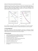
The average Nusselt number for each of the air layer thickness is showed in the Figure 3. For
values below the optimal thickness only heat transfer by conduction is presented and the
Nusselt number is equal to the unit. In agreement with equation (10), the effective
conductivity is equal to the conductivity of the air. When
L > 0.02 m the Nusselt number is
bigger than unity, this result corresponds to the heat transfer by natural convection, where
the cellular flow patterns produces an increase in the heat transfer coefficient due to the
temperature gradient applied.


-0.5
-0.4
-0.3
-0.2
-0.1
0
0.1
0.2
0.3
0.4
0.5
0.0 0.1 0.2 0.3 0.4 0.5 0.6 0.7 0.8 0.9
1.0
Velocity (m/s)
Adimensional thickness
8 [ 1 ]
10 [ 1 ]

(a)

-0.5
-0.4
-0.3
-0.2
-0.1
0
0.1
0.2
0.3
0.4
0.5
0.0 0.1 0.2 0.3 0.4 0.5 0.6 0.7 0.8 0.9 1.0
Adimensional thickness
Velocity (m/s)
8 [ 4 ] 10 [ 4 ]

(b)
Fig. 4. Velocity profile in the air layer: (a) without partitions and (b) with four partitions.
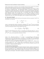
After the optimal thickness has been determined, new thicknesses of the air layer are
introduced to reduce the heat losses through multi-layer wall. These new configurations
correspond to the thicknesses of 8 and 10 cm, each one with 2, 3 or 4 partitions. In each
configuration the velocity profile was determined, in order to see the behavior of the cellular
patterns of the air inside the cavity. The Figure 4(a) shows the velocity profiles in the vertical
Heat Transfer - Mathematical Modelling, Numerical Methods and Information Technology

560
direction in the air layer for the configurations 8 [1] and 10 [1]. According to equation (8)
these configurations correspond to the air layer without partitions, where the velocity is
greater near the vertical walls and practically zero in the center of the air layer, according to

the unicellular flow pattern. For the same thicknesses, but with four partitions,
8 [4] and 10
[4]
, the velocity, Figure 4(b), shows a reduction in its values where the greatest value is near
to the hottest wall, which indicates that the heat flux by natural convection through the
multi-layer wall it is falling. In all the configurations a unicellular flow pattern is present.





4.50e-03
4.27e-03
4.05e-03
3.82e-03
3.60e-03
3.37e-03
3.15e-03
2.92e-03
2.70e-03
2.47e-03
2.25e-03
2.02e-03
1.80e-03
1.57e-03
1.35e-03
1.12e-03
9.00e-04
6.75e-04
4.50e-04

2.25e-04
0.00e+00
Aug 09,2009
FLUENT 6.2 (2d, segregated, lam)
Contours of Stream Function (kg/s)

(a)

4.50e-03
4.27e-03
4.05e-03
3.82e-03
3.60e-03
3.37e-03
3.15e-03
2.92e-03
2.70e-03
2.47e-03
2.25e-03
2.02e-03
1.80e-03
1.57e-03
1.35e-03
1.12e-03
9.00e-04
6.75e-04
4.50e-04
2.25e-04
0.00e+00
Contours of Stream Function (kg/s)

Aug 09,2009
FLUENT 6.2 (2d, segregated, lam)

(b)
Fig. 5. (a) and (b) Streamlines in the air layer.
Analysis of the Conjugate Heat Transfer in a Multi-Layer Wall Including an Air Layer

561


4.50e-03
4.27e-03
4.05e-03
3.82e-03
3.60e-03
3.37e-03
3.15e-03
2.92e-03
2.70e-03
2.47e-03
2.25e-03
2.02e-03
1.80e-03
1.57e-03
1.35e-03
1.12e-03
9.00e-04
6.75e-04
4.50e-04
2.25e-04

0.00e+00
FLUENT 6.2 (2d, segregated, lam)
Aug 09,2009
Contours of Stream Function (kg/s)

(c)




4.50e-03
4.27e-03
4.05e-03
3.82e-03
3.60e-03
3.37e-03
3.15e-03
2.92e-03
2.70e-03
2.47e-03
2.25e-03
2.02e-03
1.80e-03
1.57e-03
1.35e-03
1.12e-03
9.00e-04
6.75e-04
4.50e-04
2.25e-04

0.00e+00
Contours of Stream Function (kg/s)
FLUENT 6.2 (2d, segregated, lam)
Aug 09,2009

(d)
Fig. 5. (c) and (d) Streamlines in the air layer.
From these results it can be observed that when the velocity decreases, the heat transfer
coefficient by convection is reduced and the overall heat losses decrease. This behavior is
related to a boundary layer regime where the convection appears in the core region and the
conduction is limited to a thin boundary layer near the walls (Ganguli et al., 2009). The
Figures 5(a)-5(d) show the streamlines in the air layer, where the boundary layer regime
with the unicellular flow pattern is identified. In each configuration we can see the flow
Heat Transfer - Mathematical Modelling, Numerical Methods and Information Technology

562
patterns, where it is verified that the greater velocity is in the center of the cavity and this
one falls when the partitions are added in the air layer.
Nevertheless, the best parameter to identify the insulating effect of the air layer is the heat
transfer through the multi-layer wall. In the table 2 are shown eight configurations where
the configuration
10 [4] shows more insulating capacity, reducing the heat losses. For this
configuration each partition has a thickness near the optimal thickness. Then it is possible to
deduce that continued adding partitions with thicknesses near the optimal one, the heat
flow will fall significantly. This implies the increase in the total thickness of the wall, which
is neither practical nor advisable economically.
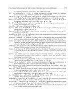
Identifying the best configuration, the temperature profiles for an air layer of 10 cm and
partitions from one to four are analyzed as shown in Figure 6. According to these profiles,
for an air layer with a single division (10 cm) the core region does not have a temperature
gradient, this behavior means that the heat transfer is controlled by the moving of the

boundary layers near the walls with a flow in a laminar boundary layer regime. The heat
transferred through the core is negligible. When the partitions in the air layer are placed, the
temperature gradients appear indicating that the heat transfer through the multi-layer wall
is present. Nevertheless, in configurations with partitions that have thicknesses bigger than
the optimal,
10[2], the temperature profiles show small gradients, a condition similar to the
air layer with a single division. When the air layer has three or four partitions,
10[3] and
10[4], the temperature profile is linear which means that in the entire air layer the heat is
transferred by conduction.


300
400
500
600
700
800
900
1000
0 0.1 0.2 0.3 0.4 0.5 0.6 0.7 0.8 0.9 1
Temperature (K)
Adimensional thickness
10 [ 1 ] 10 [ 2]
10 [ 3] 10 [ 4]



Fig. 6. Temperature profile in the air layer with different partitions.
The greatest temperature gradients appear in the air layer with four partitions, which

confirms the importance to use an air layer with partitions that have thicknesses near the
optimal. The Figures 7(a) to 7(d) show the temperature contours in the multi-layer wall,
where it can be observed that an air layer without partitions, Figure 7(a), the core to be
nearly isothermal and the heat transfer is controlled by the moving of the boundary layer
near the walls (Ganguli et al., 2009). When the thickness decreases, Figures 7(b) and 7(c), a
Analysis of the Conjugate Heat Transfer in a Multi-Layer Wall Including an Air Layer

563
steep vertical temperature gradient near the wall is present confirming the existence of the
cellular patterns and increasing the rate of the heat transfer through the air layer. With
thickness near the optimal, Figure 7(d), there is a linear temperature distribution through
the air layer and the heat transfer by conduction is dominant in that region of the thin
cavity; however, convection becomes important at the top and bottom corners of the cavity
(Ganguli et al., 2009).


(a)

(b)

Fig. 7. (a) and (b) Temperature contours in the multi-layer wall.
Heat Transfer - Mathematical Modelling, Numerical Methods and Information Technology

564

(c)

(d)
Fig. 7. (c) and (d) Temperature contours in the multi-layer wall.
5. Conclusions

In the study of the conjugate heat transfer in multi-layer walls, an optimal thickness was
identified, also the number of partitions required to reduce the heat losses and obtain a
greater insulating capability of the wall was determined. These walls were analyzed for
operating conditions of the furnaces used to bake ceramic.
Analysis of the Conjugate Heat Transfer in a Multi-Layer Wall Including an Air Layer

565
An air layer with a thickness near 3 cm allows the minimal heat transfer loss; whereas the
thickness of the other components of the multi-layer wall is constant since their size
depends on the commercial dimensions of the materials used.
According to the temperature gradient through the multi-layer wall in a furnace, an air layer
with vertical partitions reduces heat losses when the partitions have a thickness near the
optimal one; this condition reduces the fuel consumption and the pollutant emissions. For
example, the air layer of 10 cm with four partitions reduces about of 44% the heat flux
through the wall, with respect to a single air layer with the same thickness.
The reduction of the heat flux from the furnace is considerable and the cost that implies to
have an air layer with partitions is less than the cost of using a thermal insulator. In
addition, when incorporating an air layer of 10 cm with four partitions, the total thickness of
the multi-layer wall is 52 cm, which is a typical thickness of the wall in the furnaces used for
baking the ceramics. Also the energy savings make a significant contribution to the
optimization of the baking process, reducing production costs.
6. References
Aydin O. (2000). Determination of optimum air-layer thickness in double-pane windows.
Enegy and Building, 32, 303-308, ISSN: 0378-7788.
Aydin O. (2006). Conjugate heat transfer analysis of double pane windows.
Building and
Environment
, 41, 109-116, ISSN: 0360-1323.
Balderas B. A.; Gallegos M. A.; Riesco Ávila J.M.; Violante Cruz C. & Zaleta Aguilar A.
(2007). Analysis of the conjugate heat transfer in a multi-layer wall: industrial

application.
Proceedings of the XIII International Annual Congress of the SOMIM. 869-
876, ISBN: 968-9173-02-2, México, September 2007, Durango, Dgo.
Darbandi M. & Hosseinizadeh S. F. (2007). Numerical study of natural convection in vertical
enclosures using a novel non-Boussinesq algorithm.
Numerical Heat Transfer, Part A,
52, 849-873, ISSN: 1040-7782.
Department of Energy U.S.A. (Energy Efficiency and Renewable Energy) (2004). Waste heat
reduction and recovery for improving furnace efficiency, productivity and
emissions performance.
Report DOE/GO-102004-1975, 1-8.
Fluent 6.2.16 (2007).
User’s Guide.
Ganguli A.; Pandit A. & Joshi J. (2009). CFD simulation of the heat transfer in a two-
dimensional vertical enclosure.
IChemE, 87, 711-727, ISSN: 0263-8762.
Incropera F. & DeWitt D. (1996).
Introduction to Heat Transfer, John Wiley, ISBN: 0-471-30458-
1, New York.
Lacarrière B.; Lartigueb B. & Monchouxb F. (2003). Numerical study of heat transfer in a
wall of vertically perforated bricks: influence of assembly method.
Energy and
Buildings
, 35, 229-237, ISSN: 0378-7788.
Lacarrière B.; Trombe A. & Monchoux F. (2006). Experimental unsteady characterization of
heat transfer in a multi-layer wall including air layers—application to vertically
perforated bricks.
Energy and Buildings, 38, 232-237, ISSN: 0378-7788.
Patankar S.V. (1980).
Numerical Heat Transfer and Fluid Flow, Hemisphere, ISBN: 0-07-048740-

5, New York.

Heat Transfer - Mathematical Modelling, Numerical Methods and Information Technology

566
Samboua V.; Lartiguea B.; Monchouxa F. & M. Adjb (2008). Theoretical and
experimentalstudy of heat transfer through a vertical partitioned enclosure:
application to the optimization of the thermal resistance.
Applied Thermal
Engineering
, 28, 488-498, ISSN: 1359-4311.
Violante C. (2009). Analysis of the Conjugate Heat Transfer using CFD in Multi-Layer Walls
for Brick Furnace.
Thesis.
23
An Analytical Solution for Transient Heat and
Moisture Diffusion in a Double-Layer Plate
Ryoichi Chiba
Asahikawa National College of Technology
Japan
1. Introduction
In most materials, there exists a coupling effect between heat and moisture during their
transient diffusion. In particular, the coupling effect gives a significant change in the
distributions of temperature and moisture concentration in some porous materials and resin
composites (Chang, et al., 1991). Moreover, it is known that the absorption of moisture by
hygroscopic materials under high-temperature environments causes considerable
hygrothermal stresses, and meanwhile their mechanical stiffness and strength are degraded
a great deal (Komai, et al., 1991). Therefore, it is important to predict accurately the coupled
heat and moisture diffusion behaviour within the materials in assessing the life of moisture-
conditioning building materials and resin-based structural materials such as CFRP and

GFRP in hygrothermal environments.
With regard to the transient heat and moisture diffusion problems, some researchers
conducted theoretical analyses using analytical (mathematical) or numerical techniques. For
example, Sih et al. presented analytical or numerical solutions for the coupled heat and
moisture diffusion and resulting hygrothermal stress problems (Hartranft and Sih, 1980 a)
(Hartranft and Sih, 1980 b, Sih, 1983, Sih, et al., 1980) (Sih and Ogawa, 1982) (Hartranft and
Sih, 1981) (Sih, 1983, Sih, et al., 1981). Chang et al. used a decoupling technique to obtain
analytical solutions for the heat and moisture diffusion occurring in a hollow cylinder
(Chang, et al., 1991) and a solid cylinder (Chang, 1994) subjected to hygrothermal loadings.
Subsequently, using the same technique, Sugano et al. (Sugano and Chuuman, 1993 a,
Sugano and Chuuman, 1993 b) obtained analytical solutions for a hollow cylinder subjected
to nonaxisymmetric hygrothermal loadings. All the above-mentioned papers, however,
focus on/ target a single material body.
Studies that address the coupled heat and moisture diffusion problem for composite regions
(e.g., layered bodies) are limited. Chen et al. (Chen, et al., 1992) analysed the coupled
diffusion problem in a double-layered cylinder using the FEM, which leads to time-
consuming computation. In order to improve this disadvantage, Chang et al. (Chang and
Weng, 1997) later proposed an analytical technique including Hankel and Laplace
transforms, and significantly reduced the computational time compared to the FEM
analysis. However, the exact continuity of moisture flux was not fulfilled at the layer
interface although the coupling terms were included in the governing equations.
In this chapter, under the exact continuity condition the one-dimensional transient coupled
heat and moisture diffusion problem is analytically solved for a double-layer plate subjected
Heat Transfer - Mathematical Modelling, Numerical Methods and Information Technology

568
to time-varying hygrothermal loadings at the external surfaces, and analytical solutions for
the temperature and moisture fields are presented. The solutions are explicitly derived
without complicated mathematical procedures such as Laplace transform and its inversion
by applying an integral transform technique―Vodicka’s method. For simplicity, the

diffusion problem treated here is assumed to be a one-way coupled problem, which
considers only the effect of heat diffusion on the moisture diffusion, not a fully-coupled
problem, in which heat and moisture diffusions affect each other. Since, in some real cases,
moisture-induced effect on the heat diffusion (i.e., the latent heat diffusion) is evaluated to
be insignificant (Khoshbakht and Lin, 2010, Khoshbakht, et al., 2009), this assumption is
reasonable.
Numerical calculations are performed for a double-layer plate composed of distinct resin-
based composites that the temperature and moisture concentration are kept constant at the
external surfaces (the 1st kind boundary condition). The effects of coupling terms included
in the continuity condition of the moisture flux at the layer interface on the transient
moisture distribution in the plate are quantitatively evaluated. Numerical results
demonstrate that for an accurate prediction of heat and moisture diffusion behaviour, the
coupling terms in the continuity condition should be taken into consideration.
Nomenclature
a: interface location, m
B: Biot number for heat transfer (= hl/
λ
ref
)
B*: Biot number for moisture transfer (=
χ
l/
Λ
ref
)
c: moisture capacity, kg/(kg·°M)
h: heat transfer coefficient, W/(m
2
·K)
l: total thickness, m

L: Luikov number (=
η
/
κ
ref
)
m: moisture content (= c·u), wt.%
P: Possnov number (=
ε
(T
ref
−T
0
)/(u
0
−u
ref
))
t: time, s
T: temperature, K
T : dimensionless temperature (= (T−T
0
)/(T
ref
−T
0
))
u: moisture potential, °M
u : dimensionless moisture potential (= (u
0

−u)/(u
0
−u
ref
))
x, y, z: coordinates, m
Z: dimensionless coordinate (= z/l)
χ
: moisture transfer coefficient, kg/(m
2
·s·°M)
δ
i,j
: Kronecker delta
ε
: thermogradient coefficient, °M/K
γ
: eigenvalue for temperature field
η
: moisture diffusivity, m
2
/s
κ
: thermal diffusivity, m
2
/s
κ
: dimensionless thermal diffusivity (=
κ
/

κ
ref
)
λ
: thermal conductivity, W/(m·K)
μ
: eigenvalue for moisture field
τ
: Fourier number (=
κ
ref
t/l
2
)
Λ
: conductivity coefficient of moisture content, kg/(m·s·°M)
An Analytical Solution for Transient Heat and Moisture Diffusion in a Double-Layer Plate

569
Subscripts
b: bottom surface
i: layer number
m: eigenvalue number
ref: reference value
t: top surface
0: initial
∞: surrounding medium
2. Theoretical analysis
Consider an infinite double-layer plate constructed of hygroscopic materials, which is
referred to Cartesian coordinate system as shown in Fig. 1. The total thickness of the plate is

represented by l. The quantities with subscript 1 or 2 denote those for the 1st or 2nd layer of
the double-layer plate throughout the chapter. The coordinate value a indicates the location
of the layer interface. The temperature and moisture content measured by the moisture
potential in the plate are assumed to be initially T
0
and u
0
, respectively. We denote the
temperatures of the surrounding media by functions T
t∞
(t) and T
b∞
(t) and the moisture
potentials of them by u
t∞
(t) and u
b∞
(t). The plate is subjected to these hygrothermal loadings
via heat and moisture transfer coefficients h
t
, h
b
,
χ
t
and
χ
b
.

λ
1
,
Λ
1
,
κ
1
,
η
1
,
ε
1
, c
1

λ
2
,
Λ
2
,
κ
2
,
η
2
,
ε

2
, c
2

z
x, y
0
l
a
T
t∞
(t), u
t∞
(t)
T
b∞
(t), u
b∞
(t)
h
t
,
χ
t

h
b
,
χ
b

Layer 1
Layer 2

Fig. 1. Physical model and coordinate system
For the one-dimensional case shown in Fig.1, heat and moisture move along the z axis only.
When the effect of the moisture content (or potential) gradient in the energy equation is
Heat Transfer - Mathematical Modelling, Numerical Methods and Information Technology

570
neglected, the transient heat and moisture diffusion equations for the ith layer (i = 1, 2) are
written in dimensionless form as follows (Lykov and Mikhailov, 1965):

2
2
1(,) (,)
ii
i
TZ TZ
Z
τ
τ
κτ
∂∂
=
∂∂

τ
> 0, i = 1, 2, (1a)

22
22
1(,) (,) (,)
ii i
i
i
uZ uZ TZ
P
LZZ
τ
ττ
τ
∂∂ ∂
=−
∂∂ ∂

τ
> 0, i = 1, 2. (1b)
The one-way coupled system of equations given by Eqs. (1) is equivalent to the constant
properties model presented by Fudym et al. (Fudym, et al., 2004). For constant moisture
capacity, the moisture potential u
i
and moisture content m
i
are related by m
i
= c
i
·u
i

.
The initial conditions are defined as:
( ,0) 0
i
TZ
=
;
(,0) 0
i
uZ
=
i = 1, 2. (2a,b)
At the two sides of the plate (Z = 0 and Z = 1), the mass diffusion caused by the temperature
and moisture gradients affects the mass balance (Chang and Weng, 2000 a). At the interface
between two constitutive materials, the distributions of temperature and moisture potential
are continuous and the moisture flux depending on both temperature and moisture
potential gradients must be also continuous as well as the heat flux, provided that interfacial
contact resistance is negligible. Therefore, the boundary and continuity conditions can be
given as follows:

(
)
()
1
tt 1
0,
() 0, 0
T
BT T
Z

τ
ττ
∞
∂
⎡⎤
+
−=
⎣⎦
∂
, (3a)

(
)
(
)
()
11
*
1tt1
0, 0,
() 0, 0
uT
PBuu
ZZ
ττ
ττ
∞
∂∂
−
+−⎡−⎤=

⎣⎦
∂∂
, (3b)

(
)
()
2
b
b2
1,
() 1, 0
T
BT T
Z
τ
ττ
∞
∂
⎡⎤
−
−=
⎣⎦
∂
, (3c)

(
)
(
)

()
22
*
2bb2
1, 1,
() 1, 0
uT
PBuu
ZZ
ττ
ττ
∞
∂∂
−
++⎡−⎤=
⎣⎦
∂∂
, (3d)

(
)
(
)
11 21
,,TZ TZ
τ
τ
= ;
(
)

(
)
11 21
,,uZ u Z
τ
τ
= , (4a,b)

(
)
(
)
11 21
12
,,TZ TZ
ZZ
τ
τ
λλ
∂∂
=
∂∂
, (4c)

(
)
(
)
(
)

(
)
11 11 21 21
111 2 22
,, , ,uZ TZ u Z TZ
PP
Z
ZZ Z
τ
ττ τ
∂∂∂ ∂
−Λ + Λ = −Λ + Λ
∂
∂∂ ∂
, (4d)
where Z
1
= a/l,
ref
/
ii
λ
λλ
= and
ref
/
ii
Λ
=Λ Λ . In existing analytical studies, the second terms
of both sides of Eq. (4d) were omitted because of mathematical difficulties.

An Analytical Solution for Transient Heat and Moisture Diffusion in a Double-Layer Plate

571
An analytical solution to the transient heat conduction problem expressed by Eqs. (1a), (2a),
(3a), (3c), (4a) and (4c) has already been derived by Sugano et al. (Sugano, et al., 1993) as
follows:

2
11
(,) () cos sin ( ) ()
mm
i m im im ij ij j
mj
ii
ZZ
TZ A B CZ DV
γγ
τ
φτ τ
κκ
∞
==
⎡⎤
⎛⎞ ⎛⎞
=+++⎢⎥
⎜⎟ ⎜⎟
⎜⎟ ⎜⎟
⎢⎥
⎝⎠ ⎝⎠
⎣⎦

∑∑
for i = 1, 2, (5)
where

1t
() ()VT
τ
τ
∞
=− ;
2b
() ()VT
τ
τ
∞
= , (6a, b)

2
22
0
1
d()
( ) exp( ) exp( ) d
d
j
mmmmmj
j
Vt
g
tf t

t
τ
φτ γτ γ
=
⎡
⎤
=− −
⎢
⎥
⎣
⎦
∑
∫
. (7)
The procedure for determining the eigenvalues
γ
m
(m = 1, 2,…) and the expansion
coefficients g
m
and f
mj
(j = 1, 2) can be found in (Sugano, et al., 1993). The constants A
im
, B
im
,
C
ij
and D

ij
in Eq. (5) are determined from the boundary and continuity conditions, Eqs. (3a),
(3c), (4a) and (4c).
Rewriting Eq. (1b) with Eq. (5) yields

2
2
1(,) (,)
(,)
ii
i
i
uZ uZ
QZ
LZ
ττ
τ
τ
∂∂
=+
∂∂
for i = 1, 2, (8)
where

()
2
1
,()cossin
imm
immimim

m
i
ii
PZZ
QZ A B
γγ
τγφτ
κ
κκ
∞
=
⎡
⎤
⎛⎞ ⎛⎞
=+
⎢
⎥
⎜⎟ ⎜⎟
⎜⎟ ⎜⎟
⎢
⎥
⎝⎠ ⎝⎠
⎣
⎦
∑
. (9)
The transient moisture diffusion problem for a composite medium represented by Eqs. (2b),
(3b), (3d), (4b), (4d) and (8) is analysed by extending the ideas in an integral transform
technique—Vodicka’s method (Vodicka, 1955). Using this method, the solution to the
moisture diffusion problem is obtained as

3
11
(,) () () () ()
i m im ij j
mj
uZ R Z FZW
τ
ψτ τ
∞
==
=+
∑∑
, i = 1, 2, (10)
with the following functions:

**
()
ij ij ij
FZ CZ D=+, j = 1, 2, 3, (11)

(
)
1
1
1t
*
t
0,
() ()

T
P
Wu
BZ
τ
τ
τ
∞
∂
=−
∂
for
*
t
0B
≠
,
1
() 0W
τ
=
for
*
t
0B
=
, (12a)

(
)

2
2
3b
*
b
1,
() ()
T
P
Wu
BZ
τ
τ
τ
∞
∂
=+
∂
for
*
b
0B
≠
,
3
() 0W
τ
=
for
*

b
0B
=
, (12b)
Heat Transfer - Mathematical Modelling, Numerical Methods and Information Technology

572

(
)
(
)
11 21
211 22
,,
()
TZ TZ
WP P
ZZ
τ
τ
τ
∂∂
=Λ −Λ
∂∂
. (12c)
The constants
*
ij
C and

*
ij
D are determined from the following relationships:

11 21
() ()0
jj
FZ F Z
−
= , j = 1, 2, 3, (13a)

11 21
122,
d() d()
dd
jj
j
FZ FZ
ZZ
δ
Λ−Λ = j = 1, 2, 3, (13b)

1
**
t1 t1,
d(0)
(0)
d
j
j

j
F
BF B
Z
δ
−=, j = 1, 2, 3, (13c)

2
**
b
2b3,
d(1)
(1)
d
j
j
j
F
BF B
Z
δ
+=, j = 1, 2, 3. (13d)

R
im
(Z) is the solution to the eigenvalue problem corresponding to Eqs. (3b), (3d), (4b), (4d)
and (8) and is given as follows:

**
() cos sin

mm
im im im
ii
Z
Z
RZ A B
L
L
μμ
⎛⎞ ⎛⎞
=+
⎜⎟ ⎜⎟
⎜⎟ ⎜⎟
⎝⎠ ⎝⎠
, (14)

with
μ
m
being an eigenvalue. The conditions necessary to determine the unknown constants
*
im
A
and
*
im
B
can be obtained by substituting Eqs. (10)−(14) into Eqs. (3b), (3d), (4b) and (4d)
as follows:

*
1
t1
d(0)
(0) 0
d
m
m
R
BR
Z
−
=
, (15a)

*
2
b2
d (1)
(1) 0
d
m
m
R
BR
Z
+
=
, (15b)

11 2 1
() ()
mm
R
ZRZ=
, (15c)

11 21
12
d() d()
dd
mm
R
ZRZ
ZZ
Λ=Λ
. (15d)

The eigenvalues
μ
m
(m = 1, 2,…) are obtained from the condition under which all the
*
im
A

and
*
im
B

values are nonzero and are, therefore, positive roots of the following transcendental
equation:

0
⋅
⋅=GEa , (16)
where
An Analytical Solution for Transient Heat and Moisture Diffusion in a Double-Layer Plate

573

*
t
1
m
B
L
μ
⎡
⎤
=−
⎢
⎥
⎢
⎥
⎣
⎦
G
;
1−

=
⋅EC D, (17a,b)

11
11
11
11
11 1 1
cos sin
sin cos
mm
mm m m
ZZ
LL
ZZ
LL L L
μμ
μμ μμ
⎡
⎤
⎛⎞ ⎛⎞
⎢
⎥
⎜⎟ ⎜⎟
⎜⎟ ⎜⎟
⎢
⎥
⎝⎠ ⎝⎠
=
⎢

⎥
⎛⎞ ⎛⎞
⎢
⎥
−Λ Λ
⎜⎟ ⎜⎟
⎢
⎥
⎜⎟ ⎜⎟
⎢
⎥
⎝⎠ ⎝⎠
⎣
⎦
C
, (17c)


11
22
11
22
22 2 2
cos sin
sin cos
mm
mm m m
ZZ
LL
ZZ

LL LL
μμ
μμ μμ
⎡
⎤
⎛⎞ ⎛⎞
⎢
⎥
⎜⎟ ⎜⎟
⎜⎟ ⎜⎟
⎢
⎥
⎝⎠ ⎝⎠
=
⎢
⎥
⎛⎞ ⎛⎞
⎢
⎥
−Λ Λ
⎜⎟ ⎜⎟
⎢
⎥
⎜⎟ ⎜⎟
⎢
⎥
⎝⎠ ⎝⎠
⎣
⎦
D

, (17d)

*
b
22 2
*
b
22 2
cos sin
sin cos
mm m
mm m
B
LL L
B
LL L
μμ μ
μμ μ
⎡
⎤
⎛⎞ ⎛⎞
+
⎢
⎥
⎜⎟ ⎜⎟
⎜⎟ ⎜⎟
⎢
⎥
⎝⎠ ⎝⎠
=

⎢
⎥
⎛⎞ ⎛⎞
⎢
⎥
−
⎜⎟ ⎜⎟
⎢
⎥
⎜⎟ ⎜⎟
⎢
⎥
⎝⎠ ⎝⎠
⎣
⎦
a
. (17e)
The time function
ψ
m
(
τ
) is expressed as

3
2* 2 *
0
1
d()
( ) exp( ) exp( ) ( ) d

d
j
mmmmmmj
j
Wt
g
tqt f t
t
τ
ψτ μτ μ
=
⎧
⎫
⎡⎤
⎪
⎪
=− + −
⎨
⎬
⎢⎥
⎪
⎪
⎣⎦
⎩⎭
∑
∫
, (18)
where the expansion coefficients
*
m

g
, q
m
(
τ
) and
*
mj
f
are given with Z
0
= 0 and Z
2
= 1 by

[]
1
1
23
11
*
2
2
1
() (0) ()d
() d
i
i
i
i

Z
i
ij j im
Z
ij
i
m
Z
i
im
Z
i
i
FzW R z z
L
g
Rz z
L
−
−
==
=
⎡⎤
Λ
⎢⎥
⎣⎦
=−
Λ
∑∑
∫

∑
∫
, (19a)

()
[]
1
1
2
1
2
2
1
,()d
()
() d
i
i
i
i
Z
ii im
Z
i
m
Z
i
im
Z
i

i
Qz R z z
q
R
zz
L
τ
τ
−
−
=
=
Λ
=
Λ
∑
∫
∑
∫
, (19b)

[]
1
1
2
1
*
2
2
1

() ()d
() d
i
i
i
i
Z
i
ij im
Z
i
i
mj
Z
i
im
Z
i
i
F
zR z z
L
f
R
zz
L
−
−
=
=

Λ
=
Λ
∑
∫
∑
∫
. (19c)