Vorticity and Vortex Dynamics 2011 Part 12 ppt
Bạn đang xem bản rút gọn của tài liệu. Xem và tải ngay bản đầy đủ của tài liệu tại đây (1.55 MB, 50 trang )
546 10 Vortical Structures in Transitional and Turbulent Shear Flows
(1)
y
x
z
(2) (3) (4) (5) (6)
(a)
(b)
Fig. 10.23. A global view of the vortical structures from transitional to a turbulent
boundary layer. (a) Sequence of transition. (b) Fully developed turbulence
corresponding high-speed and low-speed streaks. The averaged spanwise wave-
length of the streaks in the sub layer is typically 100 viscous lengths (up to
at least Re
θ
≈ 6000 based on momentum thickness θ). The streamwise struc-
tures are broken from time to time under influence of vortex interaction with
surrounding. They will also be reformed and strengthened around the high-
shear region through the instability mechanism as stated before. Unlike the
early stage of transition, all the aforementioned structures are now coexisting
with the background of small random eddies produced by vortex breakdown
or burst.
From the wall region to the outer edge of the boundary layer, there ap-
pear hairpin structures inclined to the wall at an angle of approximately
45
◦
(Fig. 10.23b). At lower Reynolds number, the vortices are less elongated
and more like horseshoe shaped. Low-Reynolds number simulations indicate
that they most often occur asymmetrically or even singly (sometimes named
hooks), with only occasional instances of counter-rotating pairs. At moder-
ate or relative higher Reynolds numbers, the vortices are elongated and more
hairpin-shaped.
There is a controversy on whether the hairpin vortices could remain up to
the fully developed turbulent region downstream and how large an area they
can occupy in the outer region. Head and Bandyopahyay (1981) reported that
a turbulent boundary layer is filled with hairpin vortices in their smoke tunnel
experiment; but it is not so from many other results. Thus, it might be helpful
to discuss the Reynolds-number effect on the hairpin structures.
The viscous dissipation of a vortex pair of separation λ
z
depends on the
viscous cancelation of the vorticity with opposite sign, which happens due
to the vorticity diffusion from both legs at a rate proportional to νω/λ
z
.
10.3 Vortical Structures in Wall-Bounded Shear Layers 547
The lifetime of the hairpin votices, t
life
, should be proportional to ω, λ
z
and
inversely proportional to the diffusion rate, and thus t
life
canbescaledto
λ
2
z
/ν. On the other hand, the lift-up velocity of the hairpin vortices depends on
the induced velocity caused by the mutual induction of the vortex pair and is
proportional to Γ/λ
z
, where the circulation Γ ∼ ωλ
2
z
. Furthermore, ω depends
on the wall shear, ω ∼ ∂U/∂y|
w
∼ u
τ
/δ and so the time t
p
required for the
hairpin vortices to lift up and penetrate the whole boundary layer of thickness
δ canbescaledtoδ
2
/u
τ
λ
z
. This gives t
p
/t
life
∼ δ
2
ν/u
τ
λ
3
z
. Then, since λ
z
is
known to be scaled to the viscous length ν/u
τ
, the ratio t
p
/t
life
is actually
the square of the Reynolds number, (δu
τ
/ν)
2
. This argument can at least
qualitatively explain why one observes larger number of horseshoe-shaped
structures and hairpins in transitional or relatively low-Reynolds number flows
than that of hairpin-shaped structures at high Reynolds numbers. For the
latter the time required for the hairpin vortices to lift up and penetrate to
the outer edge of the boundary layer will be much longer than their life time
and most of them would be dissipated before penetrating through the whole
layer.
The outer edge of the turbulent boundary layer consists of three dimen-
sional bulges, the turbulent/nonturbulent interface with the same scale of the
boundary-layer thickness δ. Deep irrotational valleys occur at the edges of
the bulges, through which free-stream fluid is entrained into the turbulent re-
gion (Robinson 1991b). Inside the bulges are slow over-turning motions with
a length scale of δ. They have relatively long life times compared with the
quasistreamwise vortices that form, evolve, and dissipate rapidly in the near-
wall region. These large-scale structures at the outer edge are also related to
the induced velocities of groups of hairpin heads.
The inner–outer region interaction is one of the major controversial issues
in turbulent boundary layer theories. It is now almost a common understand-
ing that the outer-region structures have a definite effect on the near-wall
production process (Praturi and Brodkey 1978; Nakagawa and Nezu 1981)
but not play a governing role (Falco 1983). The large over-turning motions
are weak, though they have influence on bursting and thus on small-scale
transition. Although the outer layer also contains energetic structures, recent
numerical experiments (Jim´enez and Pinelli 1999) have confirmed that the
essential inner-layer dynamics (y
+
< 60) can operate autonomously.
One of the interesting issues relevant to the inner–outer region interaction
is whether the large over-turning motion has important influence on the for-
mation of streamwise vortices. It was suggested (Brown and Thomas 1977;
Cantwell et al. 1978) that the successive passing of the large over-turning
motions would cause waviness of near-wall streamlines. The G¨ortler instabil-
ity on a concave boundary layer might have influence on the formation or
growing of the streamwise vortices. This suggestion is similar to the “G¨ortler-
Witting mechanism,” which conjectured that large amplitude T–S waves will
locally induce concave curvature in the streamlines and hence a G¨ortler
instability (Lesson and Koh 1985). But, by a computation on a wavy wall,
548 10 Vortical Structures in Transitional and Turbulent Shear Flows
Saric and Benmalek (1991) showed that the wall section with convex curva-
ture had an extraordinary stabilizing effect on the G¨ortler vortex so that the
net result of the whole wavy wall (or the large amplitude T–S waves) was sta-
bilizing. However, the flow waviness caused by the large over-turning motion
is not sinusoidal (or the convex and concave portions of the curvature are not
symmetrical), so the net effect of the overturning motion is still to be clarified
in the future.
10.3.5 Streamwise Vortices and By-Pass Transition
Streamwise vortices are seen in all high Reynolds number shear flows, includ-
ing free shear layers (mixing layer, wake, and jet, etc.) and wall-bounded shear
layers (boundary layer, wall jet, wall wake, etc.). In the former, the inflectional
instability leads to spanwise vortices first. A streamwise vortex is a product
of secondary instability of the existing spanwise structures. In the latter, the
streamwise vortex starts immediately after the nonlinear process starts in the
wall region, so one never sees an observable spanwise vortex. However, the
background mechanism of streamwise vortices formation is in common, both
due to sufficiently strong shear field and three-dimensional disturbances.
The processes described so far are not the only mechanism to form stream-
wise vortices. Corotating streamwise vortices can be formed in the boundary
layer on a sweepback wing due to the crossflow instability. Counter-rotating
streamwise vortices can also be formed due to centrifugal instability, such as
the Dean vortices in curved channels (Dean 1928), the G¨ortler vortices near
a concave surface (G¨ortler 1940; Drazin and Reid 1981), the Taylor vortices
between concentric cylinders with the inner one rotating, or the streamwise
vortices in the outer region of the wall jet on a convex wall, etc. Thus, stream-
wise vortices are a popular flow phenomenon in turbulent shear layers.
It has been shown in Sect. 10.3.2 that the streamwise vortices play a domi-
nant role in the self-sustaining mechanism of boundary-layer turbulence. Actu-
ally, the momentum transported by the streamwise vortices not only generates
the streaks but also account for the increase of skin friction in the turbulent
boundary layer (Orlandi and Jim´enez 1994). The dominant roles of stream-
wise vortices near the wall in turbulence production and drag generation is
now widely accepted (e.g., Kim et al. 1987). In engineering applications, the
influences of streamwise vortices in mass transfer (e.g., mixing), momentum
transfer (e.g., Reynolds shear stress and skin friction), and energy transfer
(e.g., heat transfer) are also significant. Besides, as will be discussed below,
streamwise vortices is a key mechanism in the by-pass transition to turbulence.
All of these explain why we have to pay enough attention to the specific nature
related to streamwise vortices.
Figure 10.2 has shown that traveling vortices may be detected as and
expressed by waves. This is however not the case for a steady streamwise vor-
tex. Correspondingly, the mechanism of disturbance growth related to stream-
wise vortices cannot be expressed by the growth of normal modes either.
The current understanding of the streak development is the nonmodal growth
10.3 Vortical Structures in Wall-Bounded Shear Layers 549
(transient growth) introduced in Sect. 9.1.2 and discussed in Sect. 9.2.4 in the
context of shear-layer instability, which has been shown to have potential im-
portance for studies of by-pass transition (e.g., Gustavsson 1991; Butler and
Farrel 1992).
A pair of counter rotating streamwise vortices in a boundary layer will
cause wall-normal velocity disturbance that accumulates (or grows) alge-
braically along the streamwise direction x (Fig. 10.24). Even if the stream-
wise vortices decay along x, the normal velocity disturbance could still grow
as an integrated effect. The closely related phenomenon is the occurrence of
low-speed streaks and the surrounding high shear layers. Actually we have
already come across similar phenomenon in the discussion of self-sustaining
mechanism in boundary layers (Fig. 10.18). The later breakdown of low speed
streaks occurs through a secondary instability, which is developed on the
local shear layer between high- and low-speed streaks when a critical Reynolds
number based on their size is sufficiently large (Sect. 9.1.2 and Sect. 9.2.4). If
this mechanism overwhelms the normal-mode transition, there occurs by-pass
transition.
Let us discuss in a little more detail. The T–S waves in a boundary layer
on a smooth plate will start when the Reynolds number reaches certain crit-
ical value. The disturbances with frequencies within the unstable region will
grow exponentially in the linear regime. If, by any mechanism, there occurs
a pair of relatively weak streamwise vortices, then their induced velocity dis-
turbances cannot compete with those induced by the T–S waves (the normal
mode) because the former grows algebraically. However, if the flow is stable to
normal-mode disturbances or there are sufficiently strong initial streamwise
vortices for the transient growth to be overwhelming, transition to turbulent
flow will take place without passing through the stage of exponential grow of
T–S waves. This is called by-pass transition.
The transition of the Couette flow and circular-pipe flow are good examples
where the velocity profiles are linearly stable to normal modes. Subcritical
transition in an ordinary boundary layer is another example where the T–S
y
z
x
v(x )
v(z )
Fig. 10.24. Transient growth and counter rotating vortices
550 10 Vortical Structures in Transitional and Turbulent Shear Flows
wave is linearly stable due to the low Reynolds number. For all these cases, the
transition scenario can occur only if there is a mechanism other than passing
through the exponential growth of T–S waves.
Besides, if the initial disturbance amplitude exceeds a threshold level, by-
pass transition will take place (Darbyshire and Mullin 1995; Draad et al. 1998),
such as in a boundary layer on a rough surface or a boundary layer under a
surrounding of high turbulence intensity (e.g., a turbine blade). This result is
independent of whether the shear flow is unstable to exponential growth of
wave-like disturbances. As discussed above, a boundary layer subjected to a
free-stream turbulence of moderate levels would develop unsteady streamwise
oriented streaky structures with high and low streamwise velocity. This phe-
nomenon was observed even as early as Klebanoff et al. (1962) who observed
a by-pass of linear stage whenever the initial amplitude of the perturbation
was large, and also discovered the existence of streamwise vortices in the flow
field near the surface by measuring two velocity components. Subcritical tran-
sitions have recently been investigated in more detail for a variety of flows,
for examples, in circular pipes (e.g., Morkovin and Reshotko 1990; Morkovin
1993; Reshotko 1994), in plane Poiseuille flows and in boundary layer flows
(e.g., Nishioka and Asai 1985; Kachanov 1994; Asai and Nishioka 1995, 1997;
Asai et al. 1996; Bowles 2000).
10.4 Some Theoretical Aspects
in Studying Coherent Structures
Having seen the significant role of coherent structures in the development of
the two example flows, their physical understanding, prediction, and control
have become a very active area in turbulence studies. However, a turbulent
flow is full of vortical structures of various scales, which can all cause the
stretching or tilting of local vorticity. It is not an easy job to calculate all
these influences unless a direct numerical simulation is performed, which up
to now is still limited to relatively low Reynolds number flows. Thus, the
traditional way in turbulence studies is the statistical method.
The famous Kolmogorov (1941, 1962) theory and the recent development
of the universal scaling law of cascading (She and Leveque 1994; She 1997,
1998) belong to the statistical method. They both revealed the multiscale
structures in turbulence and contributed firmly to the physical background of
cascading. Recently, the latter theory has made progresses in combining the
knowledge of their universal scaling law with those of coherent structures in
shear flows (Gong et al. 2004). However, there is still a long way to go before it
can help turbulence modeling to solve the problem of turbulence development
in a flow field. So, the most convenient statistical method to date is still based
on the Reynolds decomposition.
As has been pointed out in the context of Fig. 10.2 and Sect. 10.3.5, turbu-
lent disturbances related to steady components of streamwise vortices cannot
10.4 Some Theoretical Aspects in Studying Coherent Structures 551
be expressed by the temporal fluctuations of the velocity field. This brings
us to a further discussion on the limitation of the Reynolds decomposition. A
combination of triple decomposition and vortex dynamics has shed light on
building up statistical vortex dynamics and may be a more powerful way out
in turbulence studies. But more detailed studies on the vortical structures in
turbulence require DNS or deterministic theories.
Many achievements have been made on the relevance of vortex dynamics
to turbulence. Theoderson (1952) was the first to predict theoretically the
generation of hairpin-shaped structures in a boundary layer as early as 1952.
Since then, abundant experimental and computational results have been ob-
tained in the past half century, which have prepared a condition for applying
vortex dynamics to predict the coherent structures or explain their evolu-
tion (e.g., Saffman and Baker 1979; Leonard 1985; Hunt 1987; Ashurst and
Meiburg 1988; Virk and Hussain 1993; Hunt and Vassilicos 2000; Lesieur et
al. 2000; Schoppa and Hussain 2002; Lesieur et al. 2003). As mentioned in
Sect. 1.2, these efforts have naturally in turn enriched the content of vorticity
and vortex dynamics (e.g., Melander and Hussain 1993a and 1994, Pradeep
and Hussain 2000; Hussain 2002). We expect that the present section can offer
readers some brief concepts related to the basic theories that are important
in handling coherent structures.
10.4.1 On the Reynolds Decomposition
The Reynolds decomposition has been the most popularly applied statisti-
cal method and has contributed tremendously to turbulence studies. While
extended to triple decomposition of the velocity field, it has shown its poten-
tial also in studies of coherent structures.
In the triple decomposition method, one expresses any instantaneous quan-
tity ϕ as
ϕ = Φ + ϕ
c
+ ϕ
r
, (10.1)
where Φ is its time-mean, and ϕ
c
and ϕ
r
are its coherent and random compo-
nents, respectively.
Neglecting the correlation between the coherent and random motions, the
coherent energy equation can be written as (Hussain 1983)
12
U
j
∂
∂x
j
1
2
u
ci
u
ci
= −
∂
∂x
j
u
cj
p
c
+
1
2
u
ci
u
ci
u
cj
−
u
ci
u
cj
∂U
i
∂x
j
345
+
u
ri
u
rj
∂u
ci
∂x
j
−
∂
∂x
j
u
ci
u
ri
u
rj
−
c
, (10.2)
where u
i
= U
i
+ u
ci
+ u
ri
.
552 10 Vortical Structures in Transitional and Turbulent Shear Flows
The viscous diffusion term and the energy production due to normal
stresses have been neglected in (10.2) due to their little contribution to the
coherent energy balance.
The left-hand side of the equation is the advection of coherent energy
by the mean. The terms on the right-hand side are: (1) the diffusion of the
coherent energy by coherent velocity and pressure fluctuations; (2) the coher-
ent production by the mean shear; (3) the intermodal energy transfer that
expresses the rate of energy transfer from coherent motions to random ones;
(4) the diffusion of the coherent energy by random velocity fluctuations; and
(5) the viscous dissipation of coherent energy that is usually negligible.
Equation (10.2) shows very clearly the energy transfer between mean,
coherent, and random motions and is helpful in understanding, prediction,
and control of coherent structures (see Sect. 10.5.3). However, due to the prob-
lem revealed by Fig. 10.2 and discussed in Sect. 10.3.5, one should be able to
imagine that the existence of streamwise vortices would also cause problem
on both the traditional Reynolds decomposition and the triple decomposition
of the velocity field as discussed later.
The most representative product from the Reynolds decomposition is the
Reynolds shear stress −
u
v
that is a particular correlation function in turbu-
lence studies. For generality, we take the correlation function between veloc-
ity components measured at two separate points to discuss the influence of
streamwise vortices. In a statistically steady turbulence, it is defined as
R
ij
(x
k
; r, τ )=u
i
(x
k
,t)u
j
(x
k
+ r, t + τ), (10.3)
where u
i
(x
k
,t) is the instantaneous value of the ith component of the tem-
poral velocity fluctuation at position x
k
and time instant t; r and τ are
the spatial and temporal spacing between the measuring location of u
i
and u
j
respectively. The over-bar expresses time averaging. For example,
−R
12
(x
k
;0, 0) just represents the Reynolds shear stress −u
v
at location x
k
.
As is known, the correlation function can usually characterize coherent
structures in turbulent flows. However, it has a fundamental defect if stream-
wise vortices are involved. Without loss of generality, consider the simulta-
neous two-point spatial correlation of spanwise velocity components w with
spanwise spacing ∆z in a statistically two-dimensional flow, i.e., i = j = k =3
and τ = 0, that is the most characteristic quantity related to streamwise
vortices. Thus, we have:
R
33
(z; z, 0) = w
(z,t)w
(z + z,t), (10.4)
where the velocity fluctuation w
is a temporal fluctuation.
Now, the problem comes because an ideally steady streamwise vortex will
generate only a steady induced velocity, but no temporal velocity fluctuations.
Even if in real flows the so-called streamwise vortices are not entirely stream-
wise and not ideally steady, at least their steady streamwise component will
generate no temporal velocity fluctuations. Therefore, the above correlation
10.4 Some Theoretical Aspects in Studying Coherent Structures 553
function cannot reflect the full contribution of turbulence structures, espe-
cially, the influence of the steady components of streamwise vortices. Thus,
the traditional correlation function has to be reconsidered.
A possible way to express the fluctuations caused by streamwise vortices
in a statistically steady two-dimensional flow is to replace the temporal fluc-
tuations of the velocity components by spatial ones. Namely, instead of (10.4)
we set
g
33
(z;∆z, 0) = [w(z, t) −w(t)][w(z +∆z,t) −w(t)], (10.5)
where g
33
is an instantaneous value of the spatial correlation and denotes
the spanwise spatial averaging. In order to obtain a satisfactory statistical
quantity, the procedure used to obtain the instantaneous spatial correlation
function should be repeated for enough times to form an ensemble average.
In statistically steady flows, the ensemble-averaged quantity may be replaced
by a time-averaged value and we obtain
G
33
(z;∆z, 0) = (w
1
− w
av
)(w
2
− w
av
), (10.6)
where we use the following abbreviations for neatness, w
1
= w(z,t), w
2
=
w(z +∆z,t)andw
av
= w(t).
By further decomposing w
1
, w
2
, w
av
into time means and temporal fluc-
tuations, the following expression can be obtained
G
33
= w
1
w
2
+ w
1
· w
2
+ w
av
· w
av
− w
1
· w
av
− w
2
· w
av
+ w
2
av
− w
1
w
av
− w
2
w
av
, (10.7)
where w
1
and w
2
are the instantaneous values of the spanwise velocity at
location 1 and 2, respectively, w
1
and w
2
are the corresponding temporal fluc-
tuations and w
av
is the time fluctuation of w
av
. This decomposition contains
many additional terms since (10.6) is nonlinear.
In a statistically steady two-dimensional flow, w
av
= 0 at any time so that
we have
G
33
= w
1
w
2
+ w
1
· w
2
= w
1
· w
2
, (10.8)
Here w
1
and w
2
are the instantaneous values instead of the temporal velocity
fluctuations. We suggest that this G
33
is referred to as the total correlation
to distinguish it from the traditional one. If and only if the turbulent flow is
ideally two-dimensional with no steady component of w caused by streamwise
vortices, can it then recover to the traditional correlation function:
G
33
= w
1
w
2
. (10.9)
A comparison of the two correlation functions obtained in two extreme
cases is shown in Fig. 10.25 (Xu et al. 2000). The results in figure (a) were
taken in a wall jet at a sufficient downstream distance of the jet exit, where
554 10 Vortical Structures in Transitional and Turbulent Shear Flows
X = 150 mm, y = 0.4 mm
b = 5 mm, Uj = 21m s
-1
, U
ϱ
=0
X = 200 mm downstream of vortex generators
Conventional correlation
Total correlation
Conventional correlation
Total correlation
0
-1.00
-0.15
-0.10
-0.05
0.00
0.05
0.10
0.15
0.20
(a)
(b)
-1.75
-1.50
-1.25
0.00
0.25
0.50
0.75
1.00
1.25
20 40 60 80
DZ mm
100 120 140 160
0 20406080
DZ mm
100
G
33
G
33
120 140 160
Fig. 10.25. The conventional and total correlation. (a) The correlation coefficient
in a two-dimensional wall jet. (b) The correlation coefficient in a two-dimensional
boundary layer with a spanwise row of symmetrical vortex generators (wavelength =
70 mm). From Xu et al. (2000)
the turbulence was almost statistically steady and two-dimensional. The two
curves computed by conventional and total correlations are almost identical. It
indicates that even if there were streamwise vortices in the flow, they migrated
or appeared and disappeared in a random way so that the streamwise vortices
did not cause significant steady component of w. Figure (b) shows the opposite
extreme where the results were obtained in a boundary layer with a row of
symmetrical vortex generators, which were so arranged that all odd-number
generators were tilted to one side at a given angle relative to the x-axis and
those in even numbers were in the opposite side and symmetrical to the former.
10.4 Some Theoretical Aspects in Studying Coherent Structures 555
The total correlation reaches the level of O(1) while the conventional one is
very low in spite of the existence of strong streamwise vortices along with
their steady component.
In a real turbulent flow region, the steady component of streamwise vor-
tices could vary between these two extreme experimental conditions. On
the relatively more serious side, for example, Saric (1994) points out that
the G¨ortler-vortex motion produces a situation in spatially developing flows
where the disturbance is inseparable in three dimensions from the basic-state
motion and that it seems as if all interesting phenomena associated with
G¨ortler vortices share this three-dimensional inseparability. Actually, they are
only inseparable from the time-mean value because the disturbances them-
selves involve steady components. On the less serious side, for example, in a
turbulent boundary layer, the streamwise vortices have limited lifetime, within
which there would be more obvious steady component, but less or even none
in long time average (Bernard et al. 1993). This is believed to be the rea-
son why this problem did not attract enough attention and people have been
confined to the conventional correlation in turbulence studies for so long.
Since the Reynolds stresses −ρ
u
v
, −ρv
w
, −ρu
w
, and turbulence
energy −ρ
u
u
, −ρv
v
, −ρw
w
, etc. are all correlation functions, a logical
extension of the above argument is that inherent defect may exist in the
traditional concept on turbulence quantities based solely on the Reynolds
decomposition. Within that framework, all turbulence quantities are expressed
only in terms of temporal fluctuations and are supposed to represent all the
actions that the turbulence adds to the mean field. The major efforts of the
traditional turbulence modeling have been trying to model these quantities.
However, once the steady component of streamwise vortices appears, the tra-
ditional definition of turbulence energy and turbulent shear stresses will miss
an invisible fraction. This is believed to be one of the basic reasons for the
difficulties in modeling the wall region where the streamwise vortices are so
critical.
One might argue that there is nothing wrong with the Reynolds equation.
The lost fraction of turbulence contained in the steady components of stream-
wise vortices should enter the mean field. This is true. But in doing so the
steady components of the streamwise turbulence structures are not expressed
as turbulence. Many physical and technical problems would then follow. For
example, the entire concept based on the turbulence energy equation has to
be reconsidered. How can one count the turbulence production, advection,
diffusion, and dissipation if the steady component of the streamwise vortic-
ity has to be ruled out from turbulence? Besides, if one tried to absorb the
steady component of the streamwise vortices into mean flow, the traditional
Reynolds-averaged Navier–Stokes (RANS) solution for the mean field of a
nominally two-dimensional turbulent flow would become three-dimensional
and hence lose its simplicity.
As the above total correlation suggests, one of the ways out could be to ap-
ply both temporal decomposition and spatial decomposition in the spanwise
556 10 Vortical Structures in Transitional and Turbulent Shear Flows
direction to the velocity. In this way, both temporal fluctuation and the time-
mean effect of the streamwise vortices will be counted into turbulence quan-
tities. Further studies are desired before a full solution of this problem can be
reached.
10.4.2 On Vorticity Transport Equations
An alternative or even more powerful approach in studying coherent structures
might be the statistical vorticity dynamics. Instead of applying the Reynolds
decomposition and triple decomposition to the velocity field only, the statisti-
cal vorticity dynamics applies the triple decompositions to both velocity and
vorticity field:
u(x, t)=U(x, t)+u
c
(x, t)+u
r
(x, t),
(10.10)
ω(x, t)=Ω(x)+ω
c
(x, t)+ω
r
(x, t),
where u, ω are the instantaneous quantities, U , Ω are time mean quantities,
and subscripts c and r denote coherent and random constituents, respectively.
The instantaneous vorticity equation (2.168) reads
Dω
Dt
=
∂ω
∂t
+(u ·∇)ω =(ω ·∇)u + ν∇
2
ω (10.11)
indicating that the rate of change of the vorticity is due to stretching and
tilting of the vorticity caused by the instantaneous velocity gradient (the first
term) as well as to viscous diffusion (the second term). This equation can be
applied to any instantaneous velocity and vorticity field in both laminar and
turbulent flows (Sects. 3.5.1 and 3.5.3).
As the first step of applying (10.11) to coherent structures, dimensional
analysis may give a simple but important concept. Take the spanwise vortices
in a mixing layer as example. Assuming that the mean velocity difference is
of O(U ) and the thickness of the mixing layer is of O(δ), then we have the
estimates:
|ω| =O(U/δ), |∇u| =O(U/δ),
|(ω ·∇)u| =O(U
2
/δ
2
), |ν∇
2
ω| =O(νU/δ
3
). (10.12)
Hence, the ratio of the first term on the right-hand side of (10.11) to the
second term is of O(Uδ/ν), i.e., the Reynolds number based on the radial size
of large spanwise vortices, which is usually a very large number. Thus, the
development of large coherent structures in the mixing layer can be regarded
as an invicid process.
For statistical analysis, substitute (10.10) into (10.11) and take time aver-
age, we obtain the mean vorticity equation.
DΩ
Dt
=(Ω ·∇)U + ν∇
2
Ω + ∇×(u
c
× ω
c
)+∇×(u
r
× ω
r
). (10.13)
10.4 Some Theoretical Aspects in Studying Coherent Structures 557
Compared to (10.11), the first two terms on the right-hand side of (10.13) are
of the same form, but the stretching and tilting here are caused by the mean
velocity gradient only. Moreover, there occur two extra nonlinear interaction
terms on the right-hand side, which are the curl of the coherent and random
Lamb vectors and have very clear physical meaning. The third term represents
the time-averaged effect of the interaction (i.e., stretching and advection)
between the coherent vorticity and coherent velocity fluctuations. The fourth
term is the time-mean effect of the interaction between the random vorticity
and velocity fluctuations. These terms are very helpful in understanding the
development of a turbulent shear flow.
As an illustration, consider a forced mixing layer (Zhou and Wygnanski
2001). The viscous effect in (10.13) is small as discussed earlier. By assuming
that the time-mean spanwise coherent motion is basically two-dimensional
and that the influence of the random motion is negligible in a mixing layer
under two-dimensional forcing, the first and fourth terms can also be dropped
from (10.13). The rates of change of Ω from direct measurement (expressed
by symbols in Fig. 10.26) and calculated from the third term (by solid line) at
the right side of (10.13) are plotted in Fig. 10.26. The balance of data indicates
that the above assumptions are valid. Thus, DΩ/Dt is indeed dominated by
the curl of the time-mean coherent Lamb vector, including the change in the
(a)
Y(m)
0.05
0
0 1000 2000 3000 4000 5000 6000 7000
-0.05
-0.10
(c)
Y(m)
0.05
0
0 1000 2000 3000
S
-2
4000 5000
x(m)
0.22
0.38
0.66
1.06
1.26
Calc.
x(m)
0.33
0.52
0.72
0.91
1.08
1.28
1.48
Calc.
x(m)
0.32
0.47
0.59
0.80
1.00
1.20
1.40
Calc.
-0.05
-0.10
(b)
Y(m)
0.05
0
0 1000500 1500 2500 35002000 3000 4000
-0.05
-0.10
Fig. 10.26. Mean vorticity balance in a forced mixing layer (a) Forced by single
frequency, (b ) Forced by two frequencies (fundamental and subharmonic), (c) Forced
by two frequencies but with stronger amplitude. From Zhou and Wygnanski (2001)
558 10 Vortical Structures in Transitional and Turbulent Shear Flows
mean vorticity profile along the flow and the spreading of the entire mean
shear field. It also explains why the spreading rate depends on the variation
of the forcing condition.
This example clearly demonstrates the benefit of the mean vorticity equa-
tion as compared to the Reynolds equation combining with the turbulence
energy equation or the Reynolds stress transport equations. The latter can
express the interaction of mean flow field with the turbulence field or that
between turbulent velocity fluctuations themselves. The function of coher-
ent motions is buried in the turbulence fluctuations and cannot be revealed
explicitly.
For analysis of coherent motions, we assume that the coherent quanti-
ties can be represented by the phase-locked ensemble averaged quantities and
further assume that the coherent and random motions are uncorrelated. Sub-
stituting (10.10) into (10.11), taking the phase-locked ensemble average, and
neglecting the higher order quantities, the coherent vorticity equation reads
(based on Hussain 1983)
123 4
Dω
c
Dt
=(ω
c
·∇)U +(Ω ·∇)u
c
+ ν∇
2
ω
c
+ ∇·(ω
c
u
c
− ω
c
u
c
)
56 7
−∇ ·(u
c
ω
c
− u
c
ω
c
) −∇·(u
c
Ω)+∇·(ω
r
u
r
−ω
r
u
r
)
8
−∇ ·(u
r
ω
r
−u
r
ω
r
). (10.14)
where the over-bar denotes the time mean quantities and the bracket ,the
phase locked quantities. Compared to the mean vorticity equation, the first
three terms of the right side are of the same form as the first two terms of
(10.13). Instead of the stretching and tilting of the mean vorticity caused by
the mean velocity gradient in the first term of (10.13), here the first and sec-
ond terms on the right side represents the stretching/tilting of the coherent
vorticity by the mean velocity gradients and that of the mean vorticity by
the coherent velocity gradients. The third term is the viscous diffusion of the
coherent vorticity. The fourth and fifth terms represent the residual coherent
interaction (after subtracting the mean) between the coherent vorticity and
the coherent velocity fluctuations, where the summation of the time mean
components is the same as, but of the opposite sign to the third term in
(10.13). It means that while coherent interaction causes an increase of mean
vorticity, the mean coherent vorticity would be reduced by the same amount,
i.e., an energy transfer from the coherent to the mean, or vice versa. The
sixth term represents the advection of mean vorticity by the coherent velocity
fluctuations. The seventh and eighth terms involve special physical mecha-
nisms. They are the residual (after subtracting the mean) coherent interaction
between the random vorticity and velocity fluctuations. The seventh is due to
stretching and tilting, and the eighth due to advection. By these interactions,
10.4 Some Theoretical Aspects in Studying Coherent Structures 559
the coherent vorticies may be sliced into random eddies or the latter may be
reorganized into coherent ones (see Sect. 10.5.1).
As has been shown in Figs. 10.10 and 10.17b, the main mechanism of
streamwise vortices formation in a shear layer is due to the three dimensional
deformation of the spanwise vortices in a strong shear field. From the coherent
vorticity equation (10.14), this mechanism can be easily examined. Consider-
ing Dω
xc
/Dt, a small normal coherent vorticity component ω
yc
in a region of
strong mean shear ∂U/∂y will lead to a significant value of ω
yc
(∂U/∂y), and so
to a dominant first term to produce streamwise vorticity (see also Williamson
1996).
10.4.3 Vortex Core Dynamics and Polarized Vorticity Dynamics
The discussions in Sect. 10.4.2 are based on the statistic point of view. Neither
(10.13) nor (10.14) can describe any deterministic structure of the individual
coherent vortices. In order to apply vortex dynamics to study more detailed
coherent structures in turbulence, there are yet two major difficulties: the
influence of internal vorticity distribution in a vortex core on the dynamics
of the vortex is not well understood; and, the structure and dynamics of a
large-scale coherent structure in a turbulent environment are not clear. For
these purposes vortex core dynamics and polarized vorticity dynamics would
be helpful, of which the basic theories have been discussed in Sect. 8.1.2–8.1.4
(see also Melander and Hussain 1994, and Melander and Hussain 1993a).
Here, we only list some results to show their contributions in understanding
turbulence.
Figure 10.27 is a typical result from the core dynamics showing periodical
deformation of a coherent vortex core. Assume that the initial shape of a
vortex core is distorted as (A). The vorticity lines are being uncoiled because
the two ends of the vortex segment in the figure are thinner and rotate faster
Vorticity
surface
Vorticity
line
Streamline
(a) (b)
(d) (e)
(c)
Fig. 10.27. Schematic of the coupling between swirling and meridional flows. From
Melander and Hussain (1994)
560 10 Vortical Structures in Transitional and Turbulent Shear Flows
than the midportion. Meanwhile, the meridional flow induced by the vorticity
lines will continue to distort the shape of a vorticity surface sketched in the
figure further away from that of a rectilinear vortex (B). When the vorticity
lines are entirely uncoiled, the difference in rotating speed between the two
ends and the midportion is even larger so that the differential rotation causes
new coiling of the vorticity line to the opposite direction (C). Then the new
coiling with opposite sign induces a meridional flow of opposite sign and brings
the vorticity surface towards rectilinear (D). When the shape of vorticity
surface becomes rectilinear the vorticity lines are highly coiled and its induced
meridional flow causes distortion of the vortex away from rectilinear, but in
a way opposite to the original one (E), i.e., thicker and rotates slower at the
two ends than the midportion of the vortex. The dynamic procedure can be
continued in the same way as above and an oscillation of vortex shape and
coiling of vorticity lines can be easily seen. This kind of dynamic oscillation
is expected to be one of the typical behaviors of the coherent vortices in
turbulence and affects the collectively induced velocity field in turbulence. It
will also have important influence on the interaction between coherent vortices
and the surrounding random eddies.
The above oscillating mechanism is also an evidence on the coexistence of
vortices and waves in turbulence, as well as an evidence on the vortical struc-
tures as a carrier of vorticity waves (Sect. 10.1.3). While a vortex is associated
with the mass transport, a wave is the motion transfer without mass trans-
port; in many cases they are not separable. We see that generically the core
dynamics involves neither a pure wave motion nor a pure mass transport, but
a combination of both. However, in the above example, the vorticity can be
transported as waves in a vortex core without corresponding mass transport
due to the coupling between swirl and meridional flow (Hussain 1992).
Figure 10.27 has also shown that the vortices are usually polarized,
i.e.,, with a preferred swirling direction (either left-handed or right-handed,
Fig. 10.28a). Thus, the polarized vorticity dynamics (Sect. 8.1.4) becomes
an important tool in quantitative understanding of the evolution of coher-
ent structures. It can handle the problems related to mutual interactions
of the coherent structures, their coupling with fine-scale turbulence and
their break down and reorganization. The polarized vorticity equations are
shown in (8.49a) and (8.49b). Comparing with the usual vorticity equation,
these equations involve additional terms expressing that the evolution of
the one handed mode (say the left-handed) is coupled with the other (say
the right-handed). In developing the polarized vorticity dynamics, the basic
analytical tool is the complex helical wave decomposition (HWD) introduced
in Sect.2.3.4.
One of the major achievements from the polarized vorticity equation is
the structure of a coherent vortex column in an environment of random
eddies (Fig. 10.28). Due to the interaction between the coherent vortices and
the turbulence surroundings, there are always secondary structures (threads)
spun azimuthally around it. The vorticity in the threads is mostly azimuthal
10.5 Two Basic Processes in Turbulence 561
right-handed
right-handed
right-handed
(a)
(b) (c)
left-handed
left-handed
Fig. 10.28. Schematic illustration of coherent-random interaction. (a) polarized
structures, (b) primary, (c) secondary. From Melander and Hussain (1993b)
and the threads are highly polarized (Melander and Hussain 1993a and b).
It not only gives a clear view on the turbulence cascade, but also enriches
the concept of a coherent vortex: in a turbulent flow a coherent vortex should
not be only an isolated single vortex. Rather, it is always coupled with a
group of surrounding small-scale, polarized vortices winding around it. This
phenomenon also gives a good explanation of internal intermittency in tur-
bulence – the highly dissipative structures embedded into an irrotational
flow.
10.5 Two Basic Processes in Turbulence
In either a free shear layer or a wall-bounded shear layer, we have seen one
thing in common. The observed vortical structures appear as the instanta-
neous frames of mainly two developing processes. The first process starts
from a laminar/locally laminar, or a random turbulence background. Dis-
turbances of selected modes (not necessary normal modes) are growing and
lead to the formation of vortical structures with larger and larger scales. The
second process is the structural evolution in the opposite direction, i.e., the
cascade. Large coherent structures are getting smaller and smaller due to
vortex interaction and gradually pass their energy to random eddies. As the
cascade continues, the random energy will eventually dissipate to heat. From
the equations in Sect. 10.4, we can easily find out those terms representing
either process.
562 10 Vortical Structures in Transitional and Turbulent Shear Flows
10.5.1 Coherence Production – the First Process
This process is the physical source to generate and maintain a turbulence,
without which even an existing turbulence cannot survive. For example, the
turbulence generated by a grid in a uniform flow will eventually disappear
due to dissipation. This process is also the source to cause anisotropy and the
variety of the coherent structures in a turbulence field, without which even
existing coherent structures will eventually pass their energy to isotropic small
eddies.
In terms of energy transfer, this process transfers energy from the mean
to coherent energy (through instability and coherence production – second
term of (10.2)) and from random to coherent (negative intermodal transfer –
third term of (10.2)). The appearance of the organized structures as a result
of an instability mechanism was also emphasized by Prigogine (1980) from
the viewpoint of thermodynamics. As a consequence of self-organization, the
number of degrees of freedom (Lesieur 1990, p. 141) is reduced and thus
it is a procedure that leads to a negative entropy generation. In terms of
synergetics (Haken 1984), it is the process that the orderly motion evolves from
the disordered (molecular motions or random eddies) background, and hence
represents self-organization (the organization of random eddies is related to
the last two terms of (10.14)).
The self-organization of coherent vortices from random ones can be illus-
trated by two examples. One is an experiment in a rotation tank (Hopfinger
et al. 1982) where the preferred orientation of the axes of the high-vorticity
eddies are parallel to the rotation axis due to the Taylor–Proudman theorem
(see Sect. 12.1). Imagine that the rotating tank is similar to the motion of a
tornado and the surrounding eddies are the random atmospheric turbulence,
then the tornado will give the surrounding eddies a preferred orientation and
eventually strengthen the tornado. The other is a numerical study of a coher-
ent structure embedded in the surrounding fine-scale turbulence (Melander
and Hussain 1993b) as has been shown in Fig. 10.28. The small-scale random
eddies in the absence of coherent vortex are isotropic and homogeneous. The
appearance of coherent vortices destroys the isotropy by aligning the random
vortices to the swirl direction of the vortex, thereby giving the random vortices
a preferred direction, and hence increases the coherent vorticity.
We should stress here that the negative entropy generation in a turbulence
field is not in conflict with the second law of thermodynamics. The latter
asserts that the entropy is always increasing in an isolated system, but a given
turbulence region is an open system which exchanges mass and energy with
its neighboring. The given turbulence region may obtain a negative entropy
flux from its neighbor so that its entropy would be locally reduced while the
entropy in the neighboring region is increased. If the two regions add up to
be one isolated system, the total system should still have positive entropy
generation. As an interesting example from a mixing layer experiment, Huang
and Ho (1990) found that the small-scale transition was first produced by the
10.5 Two Basic Processes in Turbulence 563
strain field of the pairing vortices imposed on the streamwise vortices. The
strained streamwise vortices were unstable and initiated the random fine-
scale turbulence. That is to say, the vortex merging (with negative entropy
generation) is accompanied by the small-scale transition (with positive entropy
generation) and the total entropy generation should still be positive.
In Sects. 10.2 and 10.3, we have seen that the stability mechanism dom-
inates the coherent production. In a mixing layer, there occur typically the
Kelvin–Helmholtz instability and the formation of the spanwise vortices, the
subharmonic instability and pairing etc. In a boundary layer, there occur typ-
ically the T–S instability, the local inflectional instability and the formation of
hairpin structures, etc. They start from laminar or locally laminar background
with distributed mean vorticity (shear) and develop to organized vortices.
The background can even be turbulent; e.g., a flow field with mean shear and
filled with small eddies, where large vortices can also be produced by certain
instability mechanism. Thus, it will be interesting to discuss the similarity and
difference in applying stability theory in a turbulent and in a laminar flow.
The linear stability theory in laminar flows like those presented in Chap. 9
has been well accepted for a long history and is even taken for granted
although a so-called laminar flow is in fact full of random molecular motions.
Only because the length scale of molecular motion are so small compared to
the wavelength of the instability waves, the latter can be regarded as approxi-
mately independent of the details of time-dependent motions of fluid mole-
cules. It is this independence that ensures the physical validity of the entire
continuum mechanics including hydrodynamic stability theory. The molecu-
lar motions do have influence on the instability mechanism; they can usually
be counted by a molecular viscosity – a statistical isotropic time-mean scalar
(if without additives). Consider now a turbulence field. If the wavelength of
the concerned instability waves is much greater than the average length scale
of the background eddies, and if the latter is almost isotropic, then the sit-
uation is similar to the laminar case. The coherent instability waves may be
considered approximately independent of the details of the surrounding time-
dependent motion of the small turbulent eddies, so that the physical nature
of flow instability should work. Of course, small eddies also have influence
on the instability waves; but they could be likewise counted by certain sta-
tistical time-mean quantities such as eddy viscosity. In particular, the mean
velocity field of a mixing layer is subject to an inviscid instability. Thus, the
instability mechanism is independent of the molecular motion, or similarly,
independent of the small-scale isotropic random eddies in turbulence. That
is to say, neither molecular viscosity nor eddy viscosity affects the inviscid
instability mechanism. Thus, it is not surprising that the stability analysis for
laminar mixing layers can work very well also in turbulent mixing layers (see
details explained later).
It should be emphasized here that enough disparity in length scale is essen-
tial for the instability mechanism to be independent of the background turbu-
lence. This is true not only for the case where the length scale of background
564 10 Vortical Structures in Transitional and Turbulent Shear Flows
turbulence is much smaller than the wavelength of the instability waves as
stated above, but also for the opposite case where the length scale of the
background turbulence is much larger than the wavelength of the instability
waves. For the latter, one just needs to think about what happens in the at-
mosphere or an ocean. Miscellaneous flow instability phenomena take place
in local regions (local instability) although the whole atmosphere or ocean is
already turbulent.
The linear instability analysis was shown successful to predict the most
amplified frequencies and the amplification rates of the large spanwise vortices
in an externally excited turbulent mixing layer (Oster and Wygnanski 1982;
Monkewitz and Huerre 1982). Gaster et al. (1985) further found that their
measured disturbance matched perfectly with the linear stability calculations
in both amplitude and phase distributions in a forced turbulent mixing layer.
Morris et al. (1990, see also Roshko 2000) made a good progress in modeling
a turbulent mixing layer based on the concept that the turbulence produc-
tion is dominated by coherent production and is caused by the amplification
of the instability modes. This idea was examined by Zhou and Wygnanski
(2002) based on the data measured by Weisbrot and Wygnanski (1988). The
result from the mixing layer excited at moderate amplitude level is shown in
Fig. 10.29, where “forced by two frequencies” means forced by a fundamen-
tal frequency and its subharmonic. Figure (a) indicates that the growth rate
of the mixing layer depends directly on the turbulence production, and fig-
ure (b) indicates that the turbulence production term is indeed dominated by
the coherent production mainly related to the spanwise coherent vortices.
Though successful in the above examples, the applicability of the instabil-
ity theory in turbulence is limited. If the scales of the coherent structures of
interest are close to that of the background eddies and strong interactions hap-
pen between the two, the instability waves can no longer be independent of the
turbulence background, and thus the similarity in the instability mechanisms
between laminar and turbulent flows is no longer valid. It is also important
to mention the role of the isotropic property for the viscosity. Even in a lam-
inar flow, very small amount of the polymer additive may cause a dramatic
change in the stability character because instability wave may cause a feedback
effect on the viscosity tensor so that the growth of the instability wave is no
longer independent of molecular motions. The same is true in a turbulence
field. If the background turbulence eddies cause significant anisotropy, the
conventional stability calculation would not be applicable.
All that stated above will add complexity to a turbulent boundary layer
and make the application of stability theory in its downstream locations dif-
ficult. In a boundary layer, new vorticity is continuously sent into the flow
field and new vortical structures are continuously formed at downstream
locations, similar to what happens in a transitional boundary layer. Kachanov
(2002) described this phenomenon as a continuous transition. The downstream
flow is under the influence of background turbulent structures advected from
upstream, including organized structures like hairpins, streamwise vortices
and random vortex rings, etc. The latter may have the length scales close to
10.5 Two Basic Processes in Turbulence 565
Forced by single frequency Forced by two frequencies
Forced by two frequencies
Forced by single frequency
(a)
(c)
(b)
(d)
0.0
0.2 0.4 0.5 0.8 1.0 1.2 1.4 1.6 1.8 0.20.0 0.4 0.6 0.8 1.0 1.2 1.4 1.6
-0.02
-1.0
-0.5
-0.5
0.0
0.0
0.5
0.5
1.0
1.0
1.5
2.0
-0.01
0.00
0.01
0.02
0.03
0.04
0.05
0.5 1.0
X (m)
1.5 2.0 0.0
-0.02
-0.01
0.00
0.01
0.02
0.03
0.04
0.05
0.5 1.0
X (m)
X (m) X (m)
1.5 2.0
Fig. 10.29. The relation between growth of mixing layer and the coherent produc-
tion. (a)and(b) Growth rate versus turbulence production. Dashed line –dθ/dx;
solid line –(U
2
+ U
1
)/(U
2
− U
1
)
2
∞
−∞
(−Production)/U
2
dy;(c)and(d): Turbu-
lence production versus coherent production, where solid line – total turbulence
production, dash-dotted line – summation of the coherent production, triangle –
fundamental, square – subharmonic, and solid circle – high harmonic. From Zhou
and Wygnanski (2002)
the downstream instability waves. In addition, they are highly anisotropic. It
is believed to be the reason why so far attempts to apply instability theory in
a turbulent boundary layer has had little success except in separated bound-
ary layers, where there is a region similar to a mixing layer so that an inviscid
instability mechanism becomes dominant (see Sect. 10.6.1).
The little success in applying instability theory to analyze the whole tur-
bulent boundary layer, however, does not mean that the stability mechanism
does not exist physically in turbulent boundary layers. For example, the local
inflectional instability mechanism around low speed streaks is still a key point
in the self-sustaining mechanism of turbulence in fully developed turbulent
boundary layers.
566 10 Vortical Structures in Transitional and Turbulent Shear Flows
10.5.2 Cascading – the Second Process
This is an entropy generation process, including cascade, intermodal (coherent-
random) energy transfer (the third term of (10.2)), and dissipation. A cascade
process involves complicated iterative operation of vortex stretching, tilting
and folding (Sect. 3.5.3). However, the tendency of cascading can be explained
by a simplified sketch with only stretching involved (Fig. 10.30). Suppose that
a turbulence field is filled with many vortical structures. If a vortex filament
along the x-direction is stretched by the induction of other vortices, this
vortex filament will become thinner and rotates faster, which enhances the
local induced velocity in the y-andz-directions. This in turn increases the
local velocity gradient and causes stretching of neighboring vortices in those
directions. Consequently, the latter also becomes thinner and their rotation is
speeded up. Such a procedure will continue and every step will cause further
decrease of the length scale of the vortices. Accordingly, turbulence energy
will gradually be transferred to smaller and smaller scales.
Note that the probabilities of the cascade process as described above are
uniform in all directions, and thus the turbulent structures will approach
homogeneous and isotropic after several steps of cascade if there is no
anisotropic influence from the first process. In fact, this process exists in all
types of shear flow; and the final products of the cascade, the random eddies,
are almost the same. This is why the background random eddies in turbulent
shear flows are almost not dependent of the boundary conditions but coherent
structures are.
In a real viscous shear flow, the largest scales are usually related to the
production of coherent structures. Below that, there often exists a range of
eddy sizes called the inertial subrange. In the inertial subrange and in average
sense, no energy is added by the mean flow and no energy is taken out by vis-
cous dissipation, so that the energy flux across each wave number is constant
and the energy cascade is conservative (Tennekes and Lumley 1972). If there
is no influence from the first process, both Kolmogorov’s spectrum and She’s
universal scaling law can express the cascading very well. However, where
there is influence from an instability mechanism that causes production and
anisotropy, a variation of the similarity parameter in the She–Leveque scaling
law (She and Leveque 1994) can be seen (Gong et al. 2004).
Besides, this cascading process cannot continue unlimitedly. With the
process of stretching, thinning, and faster rotating going on, the dissipation
z
y
x
Fig. 10.30. A sketch of turbulence cascade. Based on Chen (1986)
10.5 Two Basic Processes in Turbulence 567
rate due to the molecular viscosity is greatly enhanced. (recall 2.54, 2.155 and
4.21 for the energy and enstrophy dissipation rates, their dependence on the
vorticity and its gradient, respectively). Eventually, eddies smaller than the
dissipation scale or Kolmogorov scale will be entirely dissipated with their
energy being transferred to random molecular motion, the heat, and cannot
be maintained in any turbulence field.
The dissipation scale can be directly obtained from dimensional analysis.
Experimental observations indicate that the dissipation scale η depends on
dissipation rate ε and kinematic viscosity ν. Thus we may write, dimensionally
(denoted by [ ]), [η]=[ν]
m
[ε]
n
, where [ν]=L
2
T
−1
;[η]=L;[ε]=L
2
T
−3
.
This yields m =3/4, n = −1/4, and so
[η]=[ν]
3/4
[ε]
−1/4
,η= k(ν
3
/ε)
1/4
. (10.15)
Then the Kolmogorov scale η =(ν
3
/ε)
1/4
by setting k =1.
Therefore, for a given ε , a smaller ν leads to smaller dissipation scale,
implying that smaller vortices can survive at higher Reynolds numbers. For
example, in a high Reynolds number boundary layer, the order of η can be
as small as tens of microns, and the corresponding timescale is of the order
of microseconds (Karniadakis and Choi 2003). This is why direct numerical
simulations to date are still confined to low Reynolds numbers.
The above discussion only gives an overall mechanism of cascade. Its real
physical details are miscellaneous and very complicated. Not only the vortex
stretching but also more complicated vortex interactions will be involved, such
as vortex pair instability, vortex cut-reconnection etc. as shown in Fig. 10.13
and 10.14. Furthermore, the cascading process happens often simultaneously
with the production process. Let us make use of Fig. 10.28 again to summarize
the last statements. On the one hand, it is a vivid view of fractal cascading
by the successive interactions between a coherent vortex and its surrounding
small scales. When the coherent motion defines a preferred orientation to small
random eddies, the latter are stretched in the expanse of the coherent energy.
The interaction generates further a local shear that can sustain turbulence also
in consuming the energy contained in the coherent vortex. Thus, the energy
is passed from large to secondary and continuously to even smaller scales. On
the other hand, the small scales, aligned and stretched by the coherent vortex
are self-organized into increasingly large scales through vortex merging; thus,
the interaction also involves a negative cascade or self-organization process.
10.5.3 Flow Chart of Coherent Energy and General Strategy
of Turbulence Control
Flow control in a shear layer is important in engineering applications, for
examples, lift augmentation, drag reduction, noise suppression, heat transfer,
mixing enhancement, improving combustion, or other chemical reaction, etc.
All these performances are closely related to turbulence structures. In general,
568 10 Vortical Structures in Transitional and Turbulent Shear Flows
the development of a turbulent flow depends on the generation, transfer, and
dissipation of turbulence energy (Bradshaw et al. 1967). It can be seen below,
the flow control in a shear layer is indeed a control of coherent structures,
i.e., a control of the generation, transfer, and dissipation of coherent energy.
Thus, flow control is also of interest for physical studies as a diagnostic tool
in enhancing or destruction of coherent structures.
In the coherent energy equation (10.2) the viscous dissipation of coherent
energy is usually negligible (Sect. 10.4.2). Of the rest terms, the streamwise
diffusion is relatively small, and the integrations of the two diffusion terms (by
coherent – term 1 of 10.2, and random fluctuations – term 4) across the flow
are approximately zero. Thus, the advection of the coherent energy depends
only on the two source terms, i.e., the coherent production (term 2 of 10.2)
and the intermodal (coherent-random) energy transfer (term 3). The former is
usually positive except in some limited narrow regions of certain asymmetrical
turbulent shear layers where the production could be negative (Eskinazi and
Erian 1969; Hinze 1970). The latter is usually negative except in some special
regions where self-organization mechanism becomes dominant (such as a
region where a typhoon is being formed). Thus, the main flow chart of the
coherent energy is clear. While the mean energy is being transferred to coher-
ent energy through instability mechanism, the coherent energy is transferred
to random energy through cascade. The random energy is then transferred
to the heat (the molecular energy) through dissipation. Thus, the level of
coherent energy just depends on the balance of the two processes. Although
the feedback from the random to the coherent energy always exist, such as
the reorganization of surrounding random eddies by the coherent vortices
(Fig. 10.28), it is usually of secondary importance in the energy balance.
Based on the above discussions, the basic energy chart can be expressed
schematically by Fig. 10.31, where solid lines denote the major route and the
dashed lines, the minor feedback. The water level mimics the coherent level
or the negative entropy level. The coherent production or self-organization
process that increases the negative entropy is expressed by pumps. The cas-
cading, dissipation process, and negative production are illustrated by valves.
M
p
p
C
R
H
Fig. 10.31. A flow chart of energy transfer. M – Mean energy, C – Coherent energy,
R – Random energy, H – Heat (molecular energy), P – Pump, Triangle –Valve
10.5 Two Basic Processes in Turbulence 569
Apparently the level of coherent energy in a flow just depends on how to
adjust the pumps and valves. For examples, stimulating coherent production
can lead to increase of coherent energy; suppressing it or enhancing dissipation
can reduce the level of coherent motion.
Specific methods of flow control depend on nature of the flow, purposes
of application, and techniques available. Detailed techniques are very much
different, from controlling a convectively unstable flow to a globally unstable
flow, from stimulation to suppression of coherent production, from passive to
active, from open-loop to close-loop, etc. For example, a global instability may
be stimulated very efficiently by a single sensor–actuator feedback control;
while using the same technique to suppress the global instability (where all
the global modes have to be attenuated) is difficult (Huerre and Monkwwitz
1990).
In recent two decades, amazingly large amount of studies have been con-
ducted on flow control for various purposes and with various techniques (for
reviews see, e.g., Bushnell and McGinley 1989; Fiedler and Fernholz 1990;
Gad-el-Hak 1996, 2000; Karniadakis and Choi 2003). A detailed discussion
is beyond the scope of this book. It is in order, however, to pick up a few
examples to explain the basic control strategy stated above.
Enhancement of Coherent Production
In this category, a successful example is to introduce periodical blowing on the
knee of a trailing flap to delay separation so that the lift on the wing can be
augmented (Seifert et al. 1993). Since the outer portion of the mean velocity
profile of the separated boundary layer on the flap is similar to a mixing
layer (Fig. 10.36g and Sect. 10.6.1). The periodic forcing enhanced the coherent
production of the spanwise vortices and increases the entrainment of the high-
energy fluid into the separation region. Then, if one regards the separation
region as a reservoir with the solid boundary as its one side, the streamline of
the other side will bend towards the wall due to enhanced entrainment (Katz
et al. 1989). Thus, the separation will be weakened or even eliminated.
Another example is also introducing periodical excitation at the outer edge
of the separation region of an airfoil for lift augmentation. But the physical
idea is different. The introduced disturbance is so controlled that the outer
edge of the mean separation region is bent towards and reattaches at the
trailing edge of the airfoil. The target is not to eliminate separation at large
angle of attack but to enhance the coherent production to form a series of
spanwise vortices traveling through the upper surface of the wing, so that a
strong time-mean vortex is seemingly “captured” (Fig. 10.32a) and the vortex
lift is obtained (Zhou et al. 1993).
The major criterion to distinguish the above two types of separation con-
trol is the skin friction. In the first example, the separation suppression is
targeted so that an increase of skin friction is expected as a measure of suc-
cess. But in the second example, the formation of a strong mean vortex is
570 10 Vortical Structures in Transitional and Turbulent Shear Flows
0.085 0.150 0.30
(a) (b)
0.43
C
f
ϫ 10
3
0.58 0.75 0
-4
-2
0
2
0.2 0.4 0.6
x/cx/c
y
0.8 1.0
Fig. 10.32. The mean vortex enhancement on an airfoil at large angle of attack by
periodical forcing. (α =27
◦
, Re =6.71 × 10
5
, forced with fU
∞
/c =2).(a) Mean-
velocity profile at various streamwise locations on the upper surface of the airfoil.
(b) Distribution of skin friction. In (b) open symbols – unforced; closed symbols –
forced. From Zhou et al. (1993)
expected so that a reduction of skin friction to a strong negative value is a
measure of success (Fig. 10.32b). This idea can be extended to (Zhou 1992)
and has been applied successfully in augmentation of lift in dynamic stall
(Wygnanski 1997), where, judged by the results, the dynamic stall vortex was
actually enhanced and captured in the ensemble averaged sense.
Suppression of Coherent Production
Many studies for drag reduction belong to this category (e.g., Karniadakis
and Choi 2003). Since in wall-bounded flows the sweeps and ejections in
the turbulence regeneration cycle are the major activities related to turbu-
lence production and generation of turbulent wall-shear stress (Sect. 10.3.2),
interrupting the regeneration cycle artificially should lead to large drag
reduction and even flow relaminarization, such as riblets (Walsh (1990)),
opposition control (Jacobson and Reynolds 1998), spanwise wall oscillations
(Jung et al. 1992), and spanwise traveling waves (Du et al. 2002; Zhao et al.
2004).
The opposition control is an example that offers a very clear physical
mechanism to the coherent-structure suppression. As is shown in Fig. 10.33,
the strength of near-wall streamwise vortex would be substantially reduced
by blowing and suction with normal velocities equal and opposite to that
induced by the streamwise vortex. Numerical computations have confirmed
this mechanism (Kim 2003). In experiments, the drag can be reduced by
approximately 25–30% (Choi et al. 1994).
Spanwise wall oscillation is another vivid example for the suppression of
turbulence regeneration process. The key mechanism identified is the con-
trol of the near-wall streamwise vortices and corresponding suppression of the
low-speed streak instability (Dhanak and Si 1999). Note that the spanwise lo-
cations of the low-speed streaks are at the symmetric lines of the streamwise