Radio Propagation and Remote Sensing of the Environment - Chapter 3 ppsx

© 2005 by CRC Press

53

3

Wave Propagation in
Plane-Layered Media

3.1 REFLECTION AND REFRACTION OF PLANE WAVES
AT THE BORDER OF TWO MEDIA

Natural media —



the



atmosphere, earth, and others — can be supposed to be
homogeneous only within bounded area of space. In reality, the permittivity of these
media is a function of the coordinates and, in general terms, time, which is ignored,
as a rule, because of the comparative sluggishness of natural processes. As usual,
the time required for electromagnetic wave propagation in a natural medium is much
less than typical periods of medium property changes.
In the first approximation, natural media can be considered to be plane layered;
that is, their permittivity changes in only one direction. If a Cartesian coordinates
system is chosen in such a way that one of the coordinates (for example, z) coincides
with this direction, then we may say that permittivity depends on this coordinate
only. For the atmosphere of Earth, a concept of spherical-layered media would be

more correct, and this idea is considered in the following chapters; however, we
should point out that the curvature radius of media layers of the Earth is so large
that the concept of plane stratification is sufficient in many cases.
In this chapter, we will study only plane wave propagation in plane-layered
media. We will assume waves as the plane only conventional because surfaces with
constant phase and constant amplitude are not planes in the cases of wave propaga-
tion direction inclined to the layers. On the whole, wave parameters cannot depend
on only one particular Cartesian coordinate in all cases. In most of the cases that
we will consider here, media parameters change little compared to wavelength;
therefore, surfaces of equal phase or amplitude have sufficiently large curvature radii
to be considered locally plane. It is quite acceptable to talk about plane waves in
these terms.
In some situations, medium properties can be changed sharply and on a wave-
length scale; however, regions of such great change are usually rather thin layers
and the waves are plane, outside of the layers just discussed. These layers correspond,
in the extreme, to the areas jumpy changes of permittivity and occur at the boundary
of two media. The air–ground boundary is an example of this idea.
We turn now to consideration of plane wave reflection and transmission pro-
cesses at a plane interface. We shall assume for the sake of simplicity that the
permittivity of the medium from where the wave originates is equal to unity. Air is
an example of such a medium. The problem of a wave incident on the ground from
the air is investigated in such a way. The permittivity in this case is indicated by

ε

.
The problem of wave reflection and transmission in media separated by a plane

TF1710_book.fm Page 53 Thursday, September 30, 2004 1:43 PM
© 2005 by CRC Press

54

Radio Propagation and Remote Sensing of the Environment

interface is well known and has been analyzed in many texts regarding electromag-
netic waves; therefore, we will not investigate this problem in detail here and will
examine only essential formulae.
The electrical and magnetic fields of the incident wave are described by the
vectors:
(3.1)
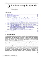
The boundary of the two media will be
assumed to be a plane that is perpendicular
to the z-axis. Let

θ

i

represent the incidence
angle (see Figure 3.1) in such a way that:
(3.2)
Note that vector

q

i

can be defined as:
(3.3)

from which it follows that w

i

=

k

sin

θ

i

.
Let us call the field excited by the incident wave in the air the

reflected wave

and represent its fields by

E

r

and

H

r

. The wave in the ground is the

refracted wave

or

transmitted wave

, and the fields of this wave are represented by

E

t

and

H

t

. It is
a simple matter to establish that the reflected and refracted waves are also found in
the plane and that their wave vectors lie in the same plane as the vector of the
incident wave. The wave vector of the reflected wave is:
(3.4)
and the wave vector of the refracted wave is:
(3.5)
The angle between vector

q

r

and the z-axis is the

angle of reflection

. It is determined
by the relation:
(3.6)
EE HH H qE
qr qr
ii
i
ii
i
iii
ee
k
ii
== =×




⋅⋅
0000
1
,, ,EEqH

iiii
k
k
00
1
= − ×




=,.q
FIGURE 3.1 Plane wave incidence
at the plane boundary.
Z
θ
i
q
i
θ
j
q
j
q
t
θ
t
cos .θ
ii
k
= −⋅

()
1
eq
z
qw ewe
ii ziz
w= −− ⋅=k
i
22
0,,
qw e
r
2
z
w=+ −
i
k
2
,
qw e
t
2
z
w= −−
i
kε
2
.
cos ,θ
rzr

= ⋅
()
1
k
eq

TF1710_book.fm Page 54 Thursday, September 30, 2004 1:43 PM
© 2005 by CRC Press

Wave Propagation in Plane-Layered Media

55

from which it follows that

θ

r

=

θ

i

; that is, the angle of reflection equals the angle
of incidence.
In the case of complex permittivity

ε

, vector

q

r

is complex and the transmitted
wave is, in general, the inhomogeneous plane wave. The refraction angle determined
from the equation:
(3.7)
is also complex in the general case. It is simple, however, to derive Snell’s law
through the formula:
(3.8)
In the case of a weak absorptive medium, when we can neglect the imaginary part
of

ε

, angle

θ

i

is real, and we can fix the propagation direction of the refracted wave.
Let us point out for later that:
(3.9)
The problem discussed here can be divided into the two cases of horizontal and
vertical polarization. In the case of horizontal polarization, the amplitudes of the

reflected and refracted waves are connected linearly with the amplitude of the
incident wave:
(3.10)
where
(3.11)
is the

coefficient of reflection

for the horizontally polarized waves, and
(3.12)
is the coefficient of transmission.
cosθ
ε
ε
ti
k
k= −⋅
()
= −
1
22
eq
zt
w
εθ θsin sin .
t
=
i
qq eeq qq eq eq

rzzt z z
= −⋅
()
= −⋅
()
+ −
()
+ ⋅
iiii
k21
2
, ε
ii
()






2
e
z
.
EEEE
rh
0
th
000
==FT

ii
,,
F
ii
ii
h
==
−−
+ −
cos sin
cos sin
θε θ
θε θ
2
2
TF
i
ii
hh
=+ =
+ −
1
2
2
cos
cos sin
θ
θε θ

TF1710_book.fm Page 55 Thursday, September 30, 2004 1:43 PM

© 2005 by CRC Press

56

Radio Propagation and Remote Sensing of the Environment

The magnetic and electrical wave components exchange places, in some sense,
for the case of vertical polarization. In this case, the equations
(3.13)
are valid, where the reflection coefficient of the vertically polarized waves is:
(3.14)
and, correspondingly, the coefficient of transmission:
(3.15)
In these equations, the coefficients

F

h

and

F

v

are referred to as the

Fresnel coefficients
of reflection

. They are complex values in the general case:
, (3.16)
and, therefore, wave reflection and refraction are accompanied not only by their
amplitude change but also by phase rotation.
Let us now express the fields of the reflected wave for the case of incidence on
the interface the plane wave of any linear polarization. For convenience, we will set
the vector of direction of the incident, reflected, and transmitted waves using the
formulae:
(3.17)
and we can obtain the expressions:
(3.18)
(3.19)
HH HH
rv tv
00 00
==FT
ii
,,
F
ii
ii
v
=
−−
+ −
εθ ε θ
εθ ε θ
cos sin
cos sin
,

2
2
TF
i
ii
vv
=+ =
+ −
1
2
2
εθ
εθ ε θ
cos
cos sin
.
FFe FFe
iF
iF
hh vv
h
v
==
arg
arg
,
qeqeqe
ii r
kk k== =,,,
rtt

Eee eE ee
ri i i
F
0
2
0
2
112−⋅
()






= ⋅
()
−⋅
()


zvz z




+ ⋅
()
{}
+

+× ⋅
eeee
eeeH
zz
h
ii
zizi
F (),
Hee eH ee
r
0
zhz z
112
2
0
2
−⋅
()






= ⋅
()
−⋅
()



ii i
F




+ ⋅
()
{}
−
− × ⋅
eeee
eeeE
zzii
vz i z i
F ()

TF1710_book.fm Page 56 Thursday, September 30, 2004 1:43 PM
© 2005 by CRC Press

Wave Propagation in Plane-Layered Media

57

for the reflected wave. A simple expression for the field amplitudes:
(3.20)
can be established from the formulae provided above. Equations (3.18) and (3.19)
can be reduced to:
(3.21)
(3.22)

We can obtain similar formulae for the transmitted wave field.
As was mentioned above, the processes of reflection and refraction are due to
changes in the radiowave amplitude and phase. In particular, the tendency is for the
reflected and refracted waves to become elliptically polarized by incidence on the
interface the plane wave of arbitrary linear polarization. In other words, a change
of the wave polarization takes place. As we already know, the polarization character
can be described by a Stokes matrix. The processes of reflection and refraction can
be considered as linear transforms; however, calculation of a Mueller matrix is rather
a complicated procedure in this case. It is easier to do direct calculation of Stokes
parameters. Let us represent the incident wave in the form ,
where the unitary vectors are directed toward the vectors of horizontal
and vertical polarization and form the coordinate basis for the coordinate system
relevant to the incident wave. We may use a the similar coordinate basis for the
reflected wave and present its field in the form
Now we will establish the relation between the orthogonal amplitude compo-
nents of the reflected and incident waves. It is easy to do this for the horizontal
components, where the required relation has the form As for the
vertical components, it is necessary to note that in this case Let us
represent the Stokes parameters of the incident wave by and the
Stokes parameters of the reflected wave by Simple calculations allow us to set
the relations between two systems of parameters and to establish the Stokes matrix
transformation law for reflection of the wave. These relations have the form:
EH
1
r
0
r
0
vz hz
z

()
=
()
=
⋅
()
+ ⋅
()
−⋅
22
20
2
20
FF
ii
eE eH
e
ee
i
()
2
EE
eE
ee
eee
rh
z
zi
zv zi
00

0
2
2
1
12=+
⋅
()
−⋅
()
−⋅
()
FF
i
i






−










++
()
⋅
()
}
FFF
hhvzii
eee,
HH
H
rv
z
zi
zh zi
00
0
2
2
1
12=+
⋅
()
−⋅
()
−⋅
()
FF
i
i
e

ee
eee






−









++
()
⋅
()
}
FFF
vhvzii
eee.
Ee e
ihh vv
=+EE
ii ii() () () ()

ee
hv
and
() ()ii
Ee e
rh
rr
v
r
v
r
=+EE
h
() () () ()
.
EFE
i
h
r
hh
() ()
.=
EFE
i
v
r
vv
() ()
.= −
Sn

n
i()
=÷
()
03
S
n
()
.
r

TF1710_book.fm Page 57 Thursday, September 30, 2004 1:43 PM
© 2005 by CRC Press

58

Radio Propagation and Remote Sensing of the Environment

(3.23a)
(3.23b)
(3.23c)
(3.23d)
Here,

Θ

r

= arg

F

h

– arg

F

v

. Similar relations can be obtained for the refracted wave.
Partial polarization appears at reflection of the noise radiation from the interface.
In particular, the coefficient of polarization has the form:
(3.24)
Let us point out, in conclusion, that if it is a question of a wave incident on a medium
with permittivity

ε

1

at the border of a medium whose permittivity equals

ε

2

, then in
all previous formulae

ε

is equal to the relative permittivity (

ε

=

ε

2

/

ε

1

), and for wave
number

k

it is necessary to substitute
Let us also mention the specific relation connecting the reflection coefficients
of vertically and horizontally polarized waves. The following relations are obtained
from Equation (3.11):
.
By inserting these expressions into the formula for the reflection coefficient of the
vertically polarized waves, we obtain the unknown relation:

(3.25)
SSFFSFF
ii
00
22
1
22
1
2
r
hv hv
() () ()
=+
()
+ −
()






,,
SSFFSFF
ii
10
22
1
22
1

2
r
hv hv
() () ()
= −
()
++
()






,,
SFFS S
ii
r232
r
hv r
() () ()
= −
()
sin cos ,ΘΘ
SFFS S
ii
332
r
hv r r
() () ()

= − +
()
cos sin .ΘΘ
m
FF
FF
=
−
+
hv
hv
22
22
.
ε
1
k.
εθ θε
θ
− =
−
+
=
+ −
+
sin cos ,
cos
2
2
1

1
122
1
i
h
i
i
F
F
FF
F
hhh
hh
()
2
F
FF
F
i
i
v
hh
h
=
−
()
−
cos
cos
.

2
12
θ
θ

TF1710_book.fm Page 58 Thursday, September 30, 2004 1:43 PM
© 2005 by CRC Press

Wave Propagation in Plane-Layered Media

59

3.2 RADIOWAVE PROPAGATION IN PLANE-LAYERED MEDIA

Now, we will consider radiowave propagation in a medium whose permittivity is,
in the general case, an arbitrary complex function of Cartesian coordinates; in this
case, we choose z. As has been pointed out, such media are referred to as plane
layered (stratified). It was noted, too, that Maxwell equations written in the form of
Equations (1.91) to (1.92) are convenient to use. These equations are simplified
essentially because

ε

=

ε

(z). Hence, it should be taken into account that a plane
wave of any polarization propagates in one plane in this case and can be represented
as the sum of two wave types. Let the y0z plane be the wave propagation plane,

which means that the field does not depend on the x-coordinate and the operator

∂

/

∂

x = 0. Then, the basic waves are E-waves (or waves of horizontal polarization),
for which the electrical field vector is directed perpendicularly to the plane of
propagation (i.e., it is represented in the form ), and H-waves (or vertical
polarized waves), for which . For E-waves, the field is described by the
equation:
(3.26)
The equation for H-waves is more complicated:
. (3.27)
Equation (3.27) differs from the wave equation but is easily reduced to it by the
substitution of :
, (3.28)
where the effective permittivity is determined by the equality:
. (3.29)
The solutions of Equations (3.26) and (3.28) we are seeking as:
(3.30)
Ee= Π
ex
He= Π
mx
∂
∂
∂

∂
ε
22
2
0
ΠΠ
Π
yz
z
22
++
()
=k .
∂
∂
∂
∂
ε
ε∂
∂
ε
22
2
1
0
ΠΠ Π
Π
m
2
m

2
m
m
xz
zz
z+ − +
()
=
d
d
k
ΠΠ
mm
=
ε
ˆ
∂
∂
∂
∂
ε
22
2
0
ˆˆ
ΠΠ
Π
m
2
m

2
m
xz
++
()
=kz
e
εε
ε
ε
e
k
d
d
= −






2
2
1
z
2
Π y,z z
y
()
=

()
Qe
ik
η
.

TF1710_book.fm Page 59 Thursday, September 30, 2004 1:43 PM
© 2005 by CRC Press

60

Radio Propagation and Remote Sensing of the Environment

Then, the problem is reduced to solution of the common differential equation:
(3.31)
The constant of separation (

η

) is determined as follows. Let us suppose that

ε

changes
with the z-coordinate beginning from some distance z

0

, and, at z z

0

,

ε

(z) =

ε

0

=

const

.
Let a plane wave described by exp[

ik

(y sin

θ

i

+ zcos

θ

i

)] be incident on the
described medium from the area z < z

0

. Thus,
(3.32)
because the incident and exited waves are both matched dependent on y.
Equation (3.31), in the general case, has no solution in the analytical form. It is
expressed through known functions only in some cases with a particular view of the
function

ε

(z). We will find one such partial solution in the next section.

3.3 WAVE REFLECTION FROM A HOMOGENEOUS
LAYER

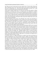
To solve the problem of waves in plane-lay-
ered media, let us first study the case of two
media with permittivities

ε

1

and

ε

3

, separated
by a homogeneous layer of thickness

d

, and
with permittivity

ε

2

(Figure 3.2). A layer of
ice floating on water is an example of such a
natural object.
It is necessary to analyze two individual
problems for E- and H-waves. Let us begin
with the E-wave by assuming that the plane
wave occurs in the semispace and
the reflected wave appears as a result of inter-
action with this layer. Let us represent poten-
tial

Π

e

in the form:
(3.33)
where

θ

i

is the incident angle. We can now describe the function

Q

e

(z) in the area
as the sum:
dQ
d
kQ
2
22
0
z
z
2
+
()

−




=
εη
.
ε
0
ηε θ
=
0
sin
i
FIGURE 3.2 Plane wave propaga-
tion in a homogeneous layer.
d
Z
1
ε
3
ε
2
ε
−∞ <<z0
Π
ee
ik
Qe

i
y,z z
y
()
=
()
εθ
1
sin
,
−∞ <<z0
Qe Fe
e
ik
e
ik
ii
z
zz
()
=+
−
εθ εθ
11
cos cos
.

TF1710_book.fm Page 60 Thursday, September 30, 2004 1:43 PM
© 2005 by CRC Press

Wave Propagation in Plane-Layered Media

61

The first term corresponds to the incident wave, for which the amplitude is assumed
to be equal to unity. The second item corresponds to the reflected wave, and

F

e

is
the coefficient of reflection.
The function

Q

e

(z) satisfies the equation:
inside the layer 0 < z <

d

and has the general solution:
Finally, in the third medium (z >

d

):

,
where

T

e

is the coefficient of transmission. The values

F

e

,

T

e

,

α

, and

β

can be defined
as solutions of equations derived from the boundary conditions.
It is useful next to employ Snell’s law by introducing the angles

θ

2

and

θ

3

:
(3.34)
If

ε

1

,

ε

2

, and

ε

3

are real numbers and if

ε

2

–

ε

1

sin

2

θ

i

> 0 and

ε

3

–

ε

1

sin

2

θ

i

> 0 (i.e.,
no total inner reflection), then these angles characterize the directions of the wave
propagation in the media considered here.
The boundary conditions, Equation (1.7), lead to continuity of function

Π

e

and
its first derivative over z at Four algebraic equations are obtained as a result:
,
Here,
(3.35)
dQ
d
kQ
e
ie

2
2
21
2
0
z
2
+ −
()
=
εε θ
sin
Qik ik
ei
zz
()
= −
()
+ −−
αεεθβ εε
exp sin exp sin
21
2
21
2
θθ
i
z
()
.

QTik
ee i
zz
()
= −
()
exp sin
εε θ
31
2
εθ εθ εθ
12233
sin sin sin .
i
==
z = 0, .d
11
122
+=+ −
()
= −
()
FF
eei
αβ ε θ εαβ θ
,cos cos
αβ εαβ θε
ϕϕ
ϕ
ϕϕ

eeTe ee
ii
e
i
ii
22
3
22
22
+= −
()
=
−−
,cos
333
3
Te
e
i
cos .
θ
ϕ
ϕεθϕεθ
222333
==kd kdcos , cos .

TF1710_book.fm Page 61 Thursday, September 30, 2004 1:43 PM
© 2005 by CRC Press

62

Radio Propagation and Remote Sensing of the Environment

Solutions to these equations have the following forms:
•For the reflection coefficient from the layer:
(3.36a)
•For the amplitudes of the directed and reflected waves inside the layer:
(3.36b)
•For the coefficient of transmission:
(3.36c)
Here,
(3.37)
is the reflection coefficient of the horizontally polarized waves from the interface of
media 1 and 2, and
(3.38)
is the corresponding coefficient of the reflection from the interface of media 2 and 3.
The same results are obtained for H-waves. It is necessary, in the previous
formulae, to substitute the reflection coefficients of horizontally polarized waves for
the equivalent ones of vertically polarized waves.
We will not analyze the general formulae, as doing so can be rather complicated.
Instead, we will confine ourselves to the particular case of a vertical wave incident
on the layer when the reflection coefficients for the E- and H-waves are similar. We
will suppose for simplicity that

ε

1

= 1; that is, assume, for example, that we have a
wave incident on the layered ground from the air. Then,

(3.39)
F
FFe
FF
e
ei
i
eie
=
()
+
()
+
() ( )
12 23
2
2
12 23
2
2
1
θθ
θθ
ϕ
e
ee
i2
2
ϕ
,

α
θ
βα θ
ϕ
ϕ
=
+
+
()
=
()
1
1
23 2
23
2
2
2
2
F
Fe
Fe
e
e
i
e
i
2
,,
T

FF e
F
e
eee
i
e
=
+
()
+
()




+
()
−
()
11
1
23
2
23
2
23
θ
θ
ϕϕ
ee

i2
2
ϕ
.
F
i
ii
i
e
12
121
2
121
θ
εθεε θ
εθεε
()
=
−−
+ −
cos sin
cos si
nn
2
θ
i
F
e
23
2

2232
2
2
2232
θ
εθεε θ
εθεε
()
=
−−
+ −
cos sin
cos si
nn
2
2
θ
FF
12
2
2
23
23
23
1
1
=
−
+
=

−
+
ε
ε
εε
εε
,.

TF1710_book.fm Page 62 Thursday, September 30, 2004 1:43 PM
© 2005 by CRC Press

Wave Propagation in Plane-Layered Media

63

Let us calculate the reflection coefficient module using the designations:
,.
(3.40)
Thus, we have:
. (3.41)
In the case of sufficiently strong absorption inside the layer (when

τ

>> 1), the reflection
coefficient is |

F

|

2

= |

F

12

|

2

, which suggests that a sufficiently thick layer — a layer
with a thickness that is many times greater then the skin depth — is equivalent to
the semispace from the point of view of the wave reflection processes. Such layers
are called

absorptive

.
We will refer to layers with moderate absorption inside as

half-absorptive

. In
these cases, the reflective coefficient module oscillates with the frequency change
due to interference of waves reflected from the layer boards. The phase shift of the
wave reflected from interfaces 2 and 3 varies with the frequency change, and, as a
result, the waves reflected from the layer boards are by turns summed in phase or

antiphase, which is why the oscillations are dependent on frequency. The amplitude
of these oscillations and their quasi-period depend on the layer thickness and its
complex permittivity. In particular, the amplitude of oscillations decreases with
increased absorption and tends to zero for the absolute absorptive layer.
Let us simplify the problem by considering the case of the dielectric layer. The
imaginary part of

ε

2

is small, and ψ
12
= π in this case. Then,
. (3.42)
Although we assume the value is small, the absorption coefficient in the layer
may be large:
(3.43)
FFe FFe
i
i
12 12 23 23
12
23
==
ψ
ψ
,,
ϕεψ
τ

22
2
==+kd i
ψτ
=
′
=
′′
kdn kdn
22
2,
F
FFe FFe
2
12
2
23
2
21223
23 12
22
1
=
++ +−
()
−−ττ
ψψ ψcos
+++ ++
()
−−

FF e FF e
12 23
2
21223
23 12
22
ττ
ψψ ψcos
F
FFe
FF e
2
12
2
23
2
2
12 23
2
1
11
1
= −
−







−






+
−τ
−−−
− +
()
21223
23
22
ττ
ψψFF e cos
′′
ε
2
τ
ε
ε
≅
′′
′
kd
2
2
TF1710_book.fm Page 63 Thursday, September 30, 2004 1:43 PM

© 2005 by CRC Press
64 Radio Propagation and Remote Sensing of the Environment
The frequency dependence of the reflection coefficient is basically determined
by the phase shift value:
(3.44)
The reflection coefficient minima are achieved at frequencies:
(3.45)
By this,
(3.46)
Maxima take place at the frequencies:
(3.47)
The maximum value of the reflection coefficient is equal to:
. (3.48)
The interference waves reflected from both interfaces is especially clear if, by using
the geometrical progression formula, we replace Equation (3.36a) by the sum:
. (3.49)
The expression reported actually represents the sum of waves reflected sequen-
tially from the layer interfaces. For example, the first item, F
12
, corresponds to
the wave reflected from the interface between the first and the second media;
ψ
ω
ε=
′
c
d
2
.
ω

ε
π
ψ
n
=
′
−






=…
()
c
d
nn
2
23
2
12,,,.
F
FFe
FF e
min
.
2
12 23
2

12 23
2
1
=
−
()
−
()
−
−
τ
τ
ω
ε
π
ψ
n
c
=
′
−






−







=…
()
d
nn
2
23
1
22
12,,,.
F
FFe
FF e
max
2
12 23
2
12 23
2
1
=
+
()
+
()
−
−

τ
τ
FF Fe FF e
i
s
s
is
s
=+
()
−
()
()
=
∞
∑
12 23 2 12 23 2
0
22
1
ϕϕ
TF1710_book.fm Page 64 Thursday, September 30, 2004 1:43 PM
© 2005 by CRC Press
Wave Propagation in Plane-Layered Media 65
represents the wave transmitted inside the layer through the first
interface and then reflected from the second interface, finally coming out after the
second interface to cross the first interface. This factor describes the wave decrease
related to the reflection from the second border, while the first one represents the
decrease caused by the dual wave passing through the first border, and, finally, the
third factor describes the phase shift appearance and corresponding wave attenuation

due to absorption with dual passing of the layer. Note that the items in Equation
(3.49) describe the waves reflected from the layer interfaces many times.
Such representation is especially convenient for describing the reflection of pulse
oscillations, for which the spectra have limited bandwidths. Let such a spectrum be
described by the function . In this instance, we will assume that we are dealing
with radar sounding the ground above, illuminating it into the nadir (in our
calculations, the z-axis is directed downward). The reflected signal form is described
by a function of the form:
. (3.50)
If we substitute Equation (3.49) here and assume that the role of the permittivity
frequency dispersion is weak in the frame of the signal bandwidth and that the
absorption in the layer does not depend on the frequency, then the result of calcu-
lations will be:
. (3.51)
Here,
is the incident field. Equation (3.51) vividly describes the processes of impulse
reflections from the layer interfaces, which we have already discussed above.
In this simple case, the reflected impulse form reiterates the form of the incident
(sounding) impulse due to the absence of the dispersion and frequency dependence
of wave attenuation due to absorption. In the opposite case, it is necessary to take
into account the dispersion signal distortion. If it is a question of natural media, then
these distortions are, as a rule, insignificant.
It is logical to establish the definition of an energetic reflective coefficient in the
case of waves with a finite-frequency bandwidth. No amplitudes of incident and
reflected waves are compared, which is senseless in the given case, but it is more
[( )]1
12 2 23 2
2
− FFe
iϕ


E
()
ω
Et E F e d
itik
z,
z
()
=
()()
−−
−∞
∞
∫

ωω ω
ω
Et F E tFFEt
ii
,z z z
()
= −
()
+ −
()







− +
12 12
2
23
1,,22
2
2
′
()
+ ⋅⋅⋅
−
ε
τ
de
Et E e d
i
itik
,z
z
()
=
()
− +
−∞
∞
∫

ωω

ω
TF1710_book.fm Page 65 Thursday, September 30, 2004 1:43 PM
© 2005 by CRC Press
66 Radio Propagation and Remote Sensing of the Environment
logical compared to their energy flows. If the following is the power flow density
of the incident wave:
then the flow density of its energy is:
. (3.52)
The Parseval equality
18
can be used for conversion from integration over time to
integration with respect to frequency. The convenience of introducing the energy
flow density is that it does not depend on time. For the reflected wave,
. (3.53)
The energetic reflective coefficient may be determined as:
. (3.54)
These formulae easily allow us to express the reflective coefficient for waves of
thermal radiation. In this case, as is known, the electromagnetic oscillations can be
represented as white noise, for which the energetic spectrum is uniform in the
frequency band (for example, ω
1
and ω
2
). Let us assume:
, (3.55)
and outside the considered frequency band. Then,
. (3.56)
S
8
E

ii
c
=
π
2
Π
ii
c
tdt
c
d=
()
=
()
−∞
∞
−∞
∞
∫∫
8
E
4
E
π
ωω
22

Π
r
4

E=
()()
−∞
∞
∫
c
Fd

ωω ω
2
F
Fd
d
i
i
i
2
2
2
==
()()
()
−∞
∞
−∞
∞
∫
∫
Π
Π

r
E
E

ωω ω
ωω

Ewhere
1
ωωωω
()
=<<
2
0
2
2
E

E ω
()
=
2
0
FFd
2
21
2
1
1
2

=
−
()
∫
ωω
ωω
ω
ω
TF1710_book.fm Page 66 Thursday, September 30, 2004 1:43 PM
© 2005 by CRC Press
Wave Propagation in Plane-Layered Media 67
So, the energetic reflective coefficient for the noise radiation is the squared module
of the common coefficient of the sine waves averaged in the frequency band.
Let us now consider the case of the dielectric layer. The result of integration in
Equation (3.56) gives:
. (3.57)
Here,
.
At a given frequency range (the difference β
2
– β
1
is constant), the energetic reflective
coefficient remains the oscillating function of the central frequency determined by
the sum ω
2
+ ω
1
; however, enlarging the frequency range (the difference β
2

– β
1
increases) results in a decrease in the amplitude of these oscillations due to the
averaging effect of summation over frequencies. This averaging becomes practically
full at β
2
– β
1
= π. Then,
(3.58)
3.4 WENTZEL–KRAMERS–BRILLOUIN METHOD
Analyzing the problems of wave propagation in stratified media, we realize that we
must solve an equation of the following type:
(3.59)
In the general case, as was pointed out, this equation has no solution open to analysis.
The corresponding solutions in known functions take place in a very limited number
of analytical dependencies, p(z); therefore, it is necessary to use approximate meth-
ods of solution of equations such as Equation (3.59), based on same peculiarities of
the function
One of these methods is the Wentzel–Kramers–Brillouin (WKB) method.
18,19
It
can be employed for the case when the scale of function p(z) changes little compared
to wavelength λ. The analytical properties of the indicated function are determined
F
A
B
B
2
21

2
2
21
2
1
1
1
= −
−
()
−
−−
()
−
ββ
ββ
β
arctan
sin
cos
ββββ
121
()
− +
()
Bcos
β
ω
ε
ψ

12
12
2
23
2
,
,
,=
′
+
c
d A
FFe
FF e
=
−






−






+

−
−
11
1
12
2
23
2
2
12 23
2
2
τ
τ
,,
B
FF e
FF e
=
+
−
−
2
1
12 23
12 23
2
2
τ
τ

FF
A
B
FFe FFe
2
0
2
2
12
2
23
2
21223
2
2
1
1
2
1
==−
−
=
+ −
−
−−ττ
FFF e
12 23
2
2−τ
.

du
d
kp u
2
2
0
z
z
2
+
()
= .
p().z
TF1710_book.fm Page 67 Thursday, September 30, 2004 1:43 PM
© 2005 by CRC Press
68 Radio Propagation and Remote Sensing of the Environment
by the analytical characteristics of the permittivity of the medium; therefore, we are
dealing conceptually with a slow change of ε(z) in the terms formulated above.
Initially, we will focus on the reasoning behind this method. For this purpose, in
the case of permanent coefficient p, the solution for the direct wave has the form
u = exp[iϕ(z)], where phase ϕ(z) = k z. Naturally, at slow behavior p(z), as was
mentioned above, the phase change at small segment dz is dϕ(z) = kdz.
The differential equation for the phase has this obvious solution:
. (3.60)
The wave amplitude in the medium with variable ε(z) cannot be constant now and
must change, but only slowly. The solution to Equation (3.59), then, is:
(3.61)
where ϕ(z) is given by Equation (3.60). By combining Equations (3.59) and (3.61),
we obtain a new equation:
(3.62)

No simplifications have been performed yet. We have just substituted one equation
for another. And, although the obtained equation is not particularly simpler, it does
allow further simplification due to the slowness concept. For this, our approach is
the same used to obtain a parabolic equation, but only the wave propagating in one
direction (in the given case, the direct one) is considered. The fast oscillated multi-
plier related to the phase change on the wavelength scale is selected in the same
manner, and corresponding equations for slow changed components are simplified.
Now, the next step of our study is to simplify Equation (3.62).
Let the scale of the permittivity change and correspondingly the function p be
equal to Λ; thus, . We may assume that the scale of change
of amplitude Q is the same. Then, it is simple enough to establish that the first item
in Equation (3.62) has a value of Q/Λ
2
, while the other terms have values of the
order Q/Λλ. It follows that the first summand may be eliminated if λ << Λ, so
(3.63)
p
p()z
ϕςςz
z
()
=
()
∫
kpd
0
uQe
i
zz
z

()
=
()
()
ϕ
,
dQ
d
ik p
dQ
d
ik
p
dp
d
Q
2
2
2
0
z
zz
2
++=.
dp d d dzz= ∝εεΛ
Q
Q
p
≅
0

14
,
TF1710_book.fm Page 68 Thursday, September 30, 2004 1:43 PM
© 2005 by CRC Press
Wave Propagation in Plane-Layered Media 69
where Q
0
is the constant. So, the solution for the direct wave is:
(3.64)
The solution for the backward wave is obtained from Equation (3.64) by replacing i by −i.
If we insert the variable σ = z/Λ into Equation (3.62), we obtain:
It is clear from this that eliminating the item with the second derivative is equivalent
to ignoring values of the order (kΛ)
–1
. This, in turn, leads to the idea that writing
the solution to Equation (3.59) in view of the Debye series:
(3.65)
is the logical deduction of the WKB approximation. Series of this kind are asymp-
totic. Inserting this series into Equation (3.59) and making equal the items with a
similar degree of wave number k give us:
(3.66)
The solution of the first equation in this formula gives us the expression for the
phase. In the process, both signs, either (+) or (–), are possible upon square root
extraction from the right side of this equation, so the independent solution of a
second-order differential equation, which Equation (3.59) is, has been taken into
account. Equation (3.66) gives us the solution to Equation (3.63), and the first items
of the Debye series correspond to the WKB approximation. Solving Equation (3.66)
allows us to determine a more precise definition of this approximation. It is easy,
however, to establish that the WKB approximation is valid by using the condition:
(3.67)

which agrees with the concept of slowness. A second condition relates to the fact
that the function p(z) has not been converted to zero, which may occur in the case
u
Q
p
ik p d≅
()








∫
0
14
0
exp .ςς
z
1
2
2
0
2
2
k
dQ
d

ip
dQ
d
i
p
dp
d
Q
Λ
σ
σσ
++ =.
ue
u
ik
ik
s
s
s
=
()
=
∞
∑
ψ
0
d
d
p
ψ

z
z






=
()
2
, 2
22
1
d
d
du
d
d
d
u
du
d
s
s
s
ψψ
zz
z
z

2
+=−
−
.
11 1
1
kkp
dp
dk
d
dΛ
∝≅<<
zzε
ε
,
TF1710_book.fm Page 69 Thursday, September 30, 2004 1:43 PM
© 2005 by CRC Press
70 Radio Propagation and Remote Sensing of the Environment
described by Equation (3.31) if somewhere ε(z) < ε
0
and angle θ
i
is such that in the
same point z
0
:
. (3.68)
The point z
0
is the turning point, and the total internal wave reflection occurs on the

plane z = z
0
. It is necessary to look for a solution more precise than the WKB
approximation for the area near the turning point. We may obtain such a solution
by using the method of reference equations.
3.5 EQUATION FOR THE REFLECTIVE COEFFICIENT
An equation for the reflective coefficient of any plane-layered medium is developed
in this part. For simplicity, let us examine the case of radio propagation along the
direction of the permittivity change. Let the z-axis coincide with this direction so
that ε = ε(z) and Maxwell’s equations can be reduced to the following:
(3.69)
Let us represent the fields of directed and reflected waves in the form:
(3.70)
Here, E
i
(z) is the field of the direct wave. The function V(z) looks like the coefficient
of reflection, although it is not literally the same. Not only is it the ratio of the
complex amplitudes of the reflected and the direct waves but it also has variable
phase correlation of type shown in Equation (3.60) for both waves. However, at
point z = 0, which is the assumed beginning of the permittivity variable, it is
transverse in the reflective coefficient. From Equations (3.69) and (3.70), it follows
that:
It follows that the function V(z) must satisfy the Riccati equation:
(3.71)
The reader can find the corresponding equations for inclined incidents of E and H
polarized waves in Breshovskish.
21
εθε
0
sin

i0
z=
()
d
d
ik
d
d
ik
E
z
H
H
z
E
x
y
y
x
==,.ε
EEz z HEz z
xy
=
()
+
()





=
()
−
()




ii
VV11,.ε
1
11
E
E
zz
i
i
d
d
V
dV
d
ik V+
()
+= −
()
ε ,
1
11
2

1
E
E
zz
i
i
d
d
V
dV
d
ik V V−
()
− =+
()
−
′
−
()
ε
ε
ε
.
dV
d
ik V V
z
= − +
′
−

()
2
4
1
2
ε
ε
ε
.
TF1710_book.fm Page 70 Thursday, September 30, 2004 1:43 PM
© 2005 by CRC Press
Wave Propagation in Plane-Layered Media 71
Equation (3.71) generally has no solutions in known functions; however, it is
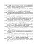
simple to solve numerically. Let us assume that permittivity is given by dependence
of the form:
(3.72)
Such dependence is depicted in
Figure 3.3. We have to suppose, because
of the assumed dependence, that if z > d
dε/dz = 0. No reflected waves are
present; therefore, V(d) = 0, which may
be formulated as the initial condition for
Equation (3.71).
In the permittivity breaking points,
the function V(z) also has a break, which
makes the numerical calculation rather
inconvenient. The function:
(3.73)
is more suitable at this point. It make sense of the medium admittance at point z
and is continuous everywhere. By substituting:

(3.74)
in Equation (3.71), we can be easily convinced that this function satisfies the
equation:
(3.75)
which is simpler than Equation (3.71) from many aspects. The initial condition for
Equation (3.75) is:
(3.76)
ε
ε
ε
ε
z
for
zfor0<z<
for
()
=
=<
()
=
∞
0
0const
d
const
,
,
>>








d.
FIGURE 3.3 Dependence of the layer
permittivity.
ε
0
ε
∞
Z
ε
(z)
ε
(z)
0
W
V
V
z
H
E
z
z
y
x
()
==

−
()
+
()
ε
1
1
,
V
W
W
z
()
=
−
+
ε
ε
dW
d
ik W
z
= −
()
ε
2
,
Wd
()
=

∞
ε ,
TF1710_book.fm Page 71 Thursday, September 30, 2004 1:43 PM
© 2005 by CRC Press
72 Radio Propagation and Remote Sensing of the Environment
and
(3.77)
replaces nonlinear Equation (3.75) with a linear one of the second order (wave
equation):
(3.78)
The boundary condition for it is:
(3.79)
The second boundary condition is not required because, in the end, we are interested
in the ratio of Equation (3.77), which is why one of the indefinite constants of the
solution to Equation (3.78) is missing. In fact, the solution generally has the form:
(3.80)
where Q
1
and Q
2
are any partial linear and independent solutions of Equation (3.78),
and A and B are constants to be determined. The function:
(3.81)
depends only on the ratio B/A, which can be obtained from Equation (3.78). The
result is:
(3.82)
If we insert this ratio into Equation (3.80) and define the reflective coefficient as:
(3.83)
W
ik

Q
Q
=
′
1
dQ
d
kQ
2
2
0
z
2
+=ε .
dQ
d
ik Q d
z
for z− ==
∞
ε 0.
QAQ BQzzz
()
=
()
+
()
12
,
W

ik
Q
B
A
Q
Q
B
A
Q
z
zz
zz
()
=
′
()
+
′
()
()
+
()
1
12
12
B
A
Qd ik Qd
Qd ik Qd
= −

′
()
−
()
′
()
−
()
∞
∞
11
22
ε
ε
.
FV
W
W
= −
()
=
−
()
+
()
0
0
0
0
0

ε
ε
,
TF1710_book.fm Page 72 Thursday, September 30, 2004 1:43 PM
© 2005 by CRC Press
Wave Propagation in Plane-Layered Media 73
then we obtain:
(3.84)
after some not very complicated calculations. Here,
Let us point out one detail. If a permittivity break occurs at the point z = 0 (i.e.,
ε(z) changes at interface), then the value of function V(0) in Equation (3.83) should
be taken at z = –0 (i.e., left of the break), and the permittivity value in Equation
(3.83) is also taken left of the break.
Finally, we will consider the case of slow permittivity variation in the layer. The
WKB method may be used for finding the functions Q
1
and Q
2
, written as:
We introduced into the WKB approximation expressions for the functions as well
as their derivatives to point out the accuracy required for their calculation (the
derivative of the permittivity is neglected in the approximation considered here).
Equation (3.82) thus can be written as:
Assumed here is the presence of a permittivity bound at the layer interface z = d.
The Fresnel coefficient of reflection is calculated according to this bound. The
function W is described by the formula:
(3.85)
It is a simple matter to discover that the main changes compared with the homoge-
neous layer are related to the substitutions:
F

YYdYYd
ZYdZYd
=
() ()
−
() ()
() ()
−
() (
21 12
12 21
00
00
))
YQikQ ZQik
ll l ll
zz zz zz z
()
=
′
()
−
() ()
=
′
()
+εε() , ()).Q
l
z
()

Q
edQ
d
ik e Q
edQ
d
i
i
i
1
14
1
14
2
14
2
== = =−
−ϕ
ϕ
ϕ
ε
ε
ε
,,,
zz
iik e
i
ε
ϕ14 −
.

B
A
d
d
eFde
id id
=
()
−
()
+
=
()
∞
∞
() ()
εε
εε
ϕϕ2
23
2
.
W
eFd
e
iid
iid
zz
z
z

()
=
()
−
()
()
−
()
()
−
(
ε
ϕϕ
ϕϕ
22
23
22
))
+
()
Fd
23
.
εεςς
εε
εε
εε
ε
z
0

z
⇒
()
=
−
+
⇒
()
=
()
−
∫
∞
dF Fd
d
,
23
23
23
23
dd
()
+
∞
ε
.
TF1710_book.fm Page 73 Thursday, September 30, 2004 1:43 PM
© 2005 by CRC Press
74 Radio Propagation and Remote Sensing of the Environment
This result is intuitive but should be regarded as a first approximation. The problem

of weak reflections will be analyzed in more detail later.
3.6 EPSTEIN’S LAYER
In this section, we will examine the case when the permittivity analytical dependence
allows the wave equation solution to be expressed in known functions, although this
is not our primary intent. The principal objective behind the problem discussed here
is to reveal the continuous transformation of the coordinate dependence of permit-
tivity from smooth to sharp and to formulate, for example, criteria for the validity
of the Fresnel coefficient application in those cases when the permittivity does not
change sharply.
The permittivity as a function of the z-coordinate is represented in the form:
(3.86)
Such dependence was considered by Epstein which is why the layer of permittivity
described here is often referred to as the Epstein layer. At ; at
If we substitute:
(3.87)
then Equation (3.78) transforms into:
.
The solutions of this equation are expressed through hypergeometric functions:
(3.88)
which has been well studied.
26
The parameters of the described functions are deter-
mined through the equalities:
(3.89)
We will not go into detail here regarding the method for solving this problem; the
interested reader can find a relevant discussion in, for example, Reference 22.
εεεεz
z
z
()

=+ −
()
+
∞00
1
e
e
d
d
.
zz→−∞ →,()εε
0
zz→∞ →
∞
,() .εε
ξ = −e
dz
,
dQ
d
dQ
d
kd
Q
2
2
22
2
0
1

1
0
ξ
ξξ
ξξ
εεξ++
−
()
−
()
=
∞
F
1
2
1
11
112
αβγξ
αβ
γ
ξ
αα ββ
γγ
ξ,,,
()
=+ +
+
()
+

()
+
()
⋅
+ ⋅⋅⋅⋅,
αβγ α ε ε
βεεγ
+=− =+
()
= −−
()
=+
∞
∞
1
12
0
0
,,
,
ikd
ikd ikd εε
0
.
TF1710_book.fm Page 74 Thursday, September 30, 2004 1:43 PM
© 2005 by CRC Press
Wave Propagation in Plane-Layered Media 75
Let us now introduce an expression for the coefficient of reflection:
(3.90)
Here, Γ(x) is the gamma-function. The obtained formula is not simple for general

analysis because of the complex behavior of the gamma-function of complex vari-
able; however, we can obtain a rather simple expression for the reflective coefficient
module, the analysis of which is not difficult. It is necessary to take into account that:
(3.91)
with the following result:
(3.92)
If πkd << 1 (thin layer), then Equation (3.92) transforms into the Fresnel formula
for the reflective coefficient. At (the layer with a slow
change of permittivity), we have:
(3.93)
It is clear that the reflective coefficient is exponentially small in the last case.
3.7 WEAK REFLECTIONS
Let us now consider the problem of a plane
wave incident from the left on the layer with
borders (Figure 3.4). The permit-
tivity changes by bound from the ε = 1 to
ε
0
at the first border of z = 0. A similar
bound from ε
d
to ε
∞
takes place at the sec-
ond border of z = d.
The permittivity varies arbitrarily but
without a sharp bound inside the area
between both interfaces. The problem of the
first approximation was already analyzed in
Section 3.5; here, we will discuss reflec-

tions inside the layer. The solution to Equa-
tion (3.71) takes the form:
F
ikd ikd ikd
=
+
()
− +
()
− +
()
∞∞
ΓΓ Γ
Γ
12 1
00 0
εεε εε[][ ]
112 1
00 0
−
()
−−
()
−−
()
∞∞
ikd ikd ikdεεε εεΓΓ[][ ]
.
ΓΓΓix
xx

ix ix
x
x
()
=+
()
−
()
=
2
11
π
π
π
πsinh
,
sinh
,
F
kd
kd
=
−
()







+
()






∞
∞
sinh
sinh
.
πε ε
πε ε
0
0
πε εkd
∞
−
()
>>
0
1
Fkd Fkd= −
()
>=−
()
<
∞∞∞

exp , exp22
00 0
πε εε πε εεif if
FIGURE 3.4 Permittivity changes in
the layer with weak reflection.
ε
ε
∞
ε
0
ε
d
1
Z
z = 0,d
TF1710_book.fm Page 75 Thursday, September 30, 2004 1:43 PM
© 2005 by CRC Press
76 Radio Propagation and Remote Sensing of the Environment
, (3.94)
where, as before, F
23
(d) is the Fresnel coefficient of reflection from the back wall
of the layer. The selection of the solution in such a form is based on physical
arguments, according to which the local reflections inside the layer are added to the
reflection from the back wall. Equation (3.71) can be reduced to the following:
(3.95)
We assume that the reflection inside the layer has to be small because of the slowness
of the permittivity changes. This assumption allows us to also assume that ℜ <<
1 and to neglect the square of this value in Equation (3.95). As a result, we obtain
the equation:

(3.96)
Now, we are dealing with a linear equation, which greatly simplifies the problem.
The solution of this equation, taking into account the condition that ℜ(d) = 0, is:
(3.97)
Here,
(3.98)
and
(3.99)
VFd e
id
zz
z
()
=
()
+ ℜ
()




()
−
()




23
2 ϕϕ

, ϕεζζz
z
()
=
()
∫
kd
0
d
d
eFe
id id
ℜ
=
′
− + ℜ
()
()
−
()




()
−
z
z
ε
ε

ϕϕ ϕϕ
4
2
23
2
2zz
()










.
d
d
Fe e
id i
ℜ
+
′
ℜ =
′
()
−
()





()
−
z
zz
ε
ε
ε
ε
ϕϕ ϕϕ
24
23
22ddid
Fe
()




()
−
()




−







23
2
2 ϕϕz
.
ℜ
()
= ℑ +
()
−
−
()
−
()
−
() ()
z
zz
ee
dL
d
ed
F
MMid M2
2

ϕς
ς
ς
ς
33
0
2
1
d
e
M
()
−






−
()
∫
z
z
.
ℑ= −
()
+
()
−

−
() () ()
∫
e
dL
d
ed
Fd
e
id M
d
Md2
23
0
2
1
ϕς
ς
ς
ς






LedM
Fde
i
i

zz
z
()
=
′
()
()
()
=
()
∫
()
1
4
0
2
23
2
ες
ες
ς
ϕς
,
ϕϕ
ϕς
ες
ες
ς
d
i

ed
()
−
()
′
()
()
∫
2
2
0
.
z
TF1710_book.fm Page 76 Thursday, September 30, 2004 1:43 PM
© 2005 by CRC Press
Wave Propagation in Plane-Layered Media 77
Now, it is a simple matter to determine the value of the reflection coefficient from
the layer:
(3.100)
Here, F
12
(0) is the Fresnel coefficient of reflection at z = 0, and we obtain:
(3.101)
A comparison with the results provided in Section 3.5 shows that the summed
reflection from the layer elements is added to the reflections from the borders when
inhomogeneous permittivity distribution occurs inside of the layer. This reflection
is described by the value ℑ according to Equation (3.101). We assume this quantity
is small, as we have neglected the square of the function ℜ(z). We also assume that
M(d) << 1 under these conditions, so:
(3.102)

The sum obtained has a clear physical sense. The first item describes the process of
direct wave local reflection. The second one describes waves generated in the process
of local reflection of the backward wave occurring due to reflection at the second
layer interface. These waves become direct, propagate to the second interface, reflect
from it, and propagate backward. This explanation allows us to understand the
proportionality of the second item to the square of the reflection coefficient F
23
(d).
We will now turn our attention to the slowness concept of permittivity variation
and the small local reflection related to it. Usually, we consider the scale of the
permittivity change to be greater than that of the wavelength; however, this require-
ment does not appear in our arguments here (based on the WKB approximation).
Our approximation is based only on the assumption of the function ℜ(z) being small;
correspondingly, the constant ℑ is also small. However, the last may be small and
by the bound, more accurately fast on the wavelength scale change of the permittivity.
By letting such a change take place from the value ε
1
to ε
3
near the point z = z on
a scale much smaller than the wavelength scale, the exponential factors in Equation
(3.102) are not changed during integration near this point, so we have:
(3.103)
F
W
W
FV
FV
=
−

()
+
()
=
()
+
()
+
() ()
10
10
00
100
12
12
.
F
FFde
FFd
id
=
()
+
()
+ ℑ




+

() ()
+
()
12 23
2
12 23
0
10
ϕ
ℑℑ




()
e
id2 ϕ
.
ℑ= −
′
()
()
+
()
−
()
()
∫
e
ed

Fde
id
i
d
2
2
0
23
2
2
4
ϕ
ϕς
ες
ες
ς
iid
i
d
ed
ϕ
ϕς
ες
ες
ς
()
−
()
′
()

()
∫
4
2
0
.
ℑ= −−
()
()
−
()




()
−
1
4
2
1
2
23
2
2
ln
ε
ε
ϕϕ ϕ
eFde

iz d idϕϕ z
()




{}
.
TF1710_book.fm Page 77 Thursday, September 30, 2004 1:43 PM