Trace Environmental Quantitative Analysis: Principles, Techniques, and Applications - Chapter 2 potx
Bạn đang xem bản rút gọn của tài liệu. Xem và tải ngay bản đầy đủ của tài liệu tại đây (2.28 MB, 82 trang )
37
2
Calibration, Verification,
Statistical Treatment of
Analytical Data, Detection
Limits, and Quality
Assurance/Quality Control
If you can measure that of which you speak, and can express it by a number, you know
something of your subject, but if you cannot measure it, your knowledge is meager
and unsatisfactory.
—Lord Kelvin
CHAPTER AT A GLANCE
Good laboratory practice 38
Error in laboratory measurement 41
Instrument calibration and quantification 45
Linear least squares regression 58
Uncertainty in interpolated linear least squares regression 64
Instrument detection limits 68
Limit of quantitation 81
Quality control 85
Linear vs. nonlinear least squares regression 91
Electronic interfaces between instruments and PCs 104
Sampling considerations 112
References 117
Chromatographic and spectroscopic analytical instrumentation are the key determi-
native tools to quantitate the presence of chemical contaminants in biological fluids
and in the environment. These instruments generate electrical signals that are related
to the amount or concentration of an analyte of environmental or environmental
health significance. This analyte is likely to be found in a sample matrix taken from
the environment, or from body fluids. Typical sample matrices drawn from the
environment include groundwater, surface water, air, soil, wastewater, sediment,
sludge, and so forth. Computer technology has merely aided the conversion of an
© 2006 by Taylor & Francis Group, LLC
38 Trace Environmental Quantitative Analysis, Second Edition
analog signal from the transducer to the digital domain. It is the relationship between
the analog or digital output from the instrument and the amount or concentration of
a chemical species that is discussed in this chapter. The process by which an electrical
signal is transformed to an amount or concentration is called instrument calibration.
Chemical analysis based on measuring the mass or volume obtained from chemical
reactions is stoichiometric. Gravimetric (where the analyte of interest is weighed)
and volumetric (where the analyte of interest is titrated) techniques are methods that
are stoichiometric. Such methods do not require calibration. Most instrumental
determinative methods are nonstoichiometric and thus require instrument calibration.
This chapter introduces the most important aspect of TEQA for the reader. After
the basics of what constitutes good laboratory practice are discussed, the concept
of instrumental calibration is introduced and the mathematics used to establish such
calibrations are developed. The uncertainty present in the interpolation of the cali-
bration is then introduced. A comparison is made between the more conventional
approach to determining instrument detection limits and the more contemporary
approaches that have recently been discussed in the literature.
1–6
These more con-
temporary approaches use least squares regression and incorporate relevant elements
from statistics.
7
Quality assurance/quality control principles are then introduced. A
contemporary statistical approach toward evaluating the degree of detector linearity
is then considered. The principles that enable a detector’s analog signal to be
digitized via analog-to-digital converters are introduced. Principles of environmental
sampling are then introduced. Readers can compare QA/QC practices from two
environmental testing laboratories. Every employer wants to hire an analyst who
knows of and practices good laboratory behavior.
1. WHAT IS GOOD LABORATORY PRACTICE?
Good laboratory practice (GLP) requires that a quality control (QC) protocol for
trace environmental analysis be put in place. A good laboratory QC protocol for any
laboratory attempting to achieve precise and accurate TEQA requires the following
considerations:
• Deciding whether an external standard, internal standard, or standard
addition mode of instrument calibration is most appropriate for the
intended quantitative analysis application.
• Establishing a calibration curve that relates instrument response to analyte
amount or concentration by preparing reference standards and measuring
their respective instrument responses.
• Performing a least squares regression analysis on the experimental cali-
bration data to evaluate instrument linearity over a range of concentrations
of interest and to establish the best relationship between response and
concentration.
• Computing the statistical parameters that assist in specifying the uncer-
tainty of the least squares fit to the experimental data points.
• Running one or more reference standards in at least triplicate as initial
calibration verification (ICV) standards throughout the calibration range.
© 2006 by Taylor & Francis Group, LLC
Calibration, Verification, Statistical Treatment 39
ICVs should be prepared so that their concentrations fall to within the
mid-calibration range.
• Computing the statistical parameters for the ICV that assist in specifying
the precision and accuracy of the least squares fit to the experimental data
points.
• Determining the instrument detection limits (IDLs).
• Determining the method detection limits (MDLs), which requires estab-
lishing the percent recovery for a given analyte in both a clean matrix and
the sample matrix. With some techniques, such as static headspace gas
chromatography (GC), the MDL cannot be determined independently
from the instrument’s IDL.
• Preparing and running QC reference standards at a frequency of once
every 5 or 10 samples. This QC standard serves to monitor instrument
precision and accuracy during a batch run. This assumes that both cali-
bration and ICV criteria have been met. A mean value for the QC reference
standard should be obtained over all QC standards run in the batch. The
standard deviation, s, and the relative standard deviation (RSD) should be
calculated.
• Preparing the running QC surrogates, matrix spikes, and, in some cases,
matrix spike duplicates per batch of samples. A batch is defined in EPA
methods to be approximately 20 samples. These reference standard spikes
serve to assess extraction efficiency where applicable. Matrix spikes and
duplicates are often required in EPA methods.
• Preparing and running laboratory blanks, laboratory control samples, and
field and trip blanks. These blanks serve to assess whether samples may
have become contaminated during sampling and sample transport.
It has been stated many times by experienced analysts that in order to achieve
GLP, close to one QC sample must be prepared and analyzed for nearly each and
every real-world environmental sample.
2. CAN DATA REDUCTION, INTERPRETATION,
AND STATISTICAL TREATMENT BE SUMMARIZED
BEFORE WE PLUNGE INTO CALIBRATION?
International Union of Pure and Applied Chemistry (IUPAC) recommendations, as
discussed by Currie,
1
is this author’s attempt to do just that. The true amount that
is present in the unknown sample can be expressed as an amount such as a #ng
analyte, or as a concentration [#µg analyte/kg of sample (weight/weight) or #µg
analyte/L of sample (weight/volume)]. The amount or concentration of true unknown
sented by τ is shown in Figure 2.1 being transformed to an electrical signal y.
accomplished. The signal y, once obtained, is then converted to the reported estimate
© 2006 by Taylor & Francis Group, LLC
Yes, indeed. Figure 2.1, adapted and modified, while drawing on recently published
present in either an environmental sample or human/animal specimen and repre-
Chapters 3 and 4 describe how the six steps from sampling to transducer are
40 Trace Environmental Quantitative Analysis, Second Edition
x
0
, as shown in Figure 2.1. This chapter describes how the eight steps from calibration
to statistical evaluation are accomplished. The ultimate goal of TEQA is then real-
ized, i.e., a reported estimate x
0
with a calculated uncertainty using statistics in the
measurement expressed as ±u. We can assume that the transduced signal varies
linearly with x, where x is the known analyte amount or concentration of a standard
reference. This analyte in the standard reference must be chemically identical to the
analyte in the unknown sample represented by its true value τ. x is assumed to be
known with certainty since it can be traced to accurately known certified reference
standards, such as that obtained from the National Institute of Standards and Tech-
nology (NIST). We can realize that
where
y
0
= the y intercept, the magnitude of the signal in the absence of analyte.
m = slope of the best-fit regression line (what we mean by regression will
be taken up shortly) through the experimental data points. The slope
also defines the sensitivity of the specific determinative technique.
e
y
= the error associated with the variation in the transduced signal for a
given value of x. We assume that x itself (the amount or concentration
of the analyte of interest) is free of error. This assumption is used
throughout the mathematical treatment in this chapter and serves to
simplify the mathematics introduced.
FIGURE 2.1 The process of trace environmental quantitative analysis. (Adapted from
L. Currie, Pure and Applied Chemistry, 67, 1699–1723, 1995.)
x
o
± u
Sampling
Sample
preservation
and storage
Extraction
Cleanup
Injection
Transducer
Calibration
Quantification
Verification
Measure IDLs
Calculate MDLs
Conduct QA/QC
Interpretation
Statistical evaluation
y
Signal (y) from transducer
that corresponds to τ; signal
may or may not include
background interferences;
requires quality analytical
instrumentation, efficient
sample preparation and
competent analytical
scientists and technicians
Reported estimate of
amount or concentration
of unknown targeted
analyte (x
0
) with
calculated uncertainty
(±u) in the
measurement; the
ultimate goal and
limitation of TEQA
True amount or
concentration (τ) of
unknown targeted
analyte in
environmental sample
or animal specimen;
satisfies a societal
need to know, the
need for TEQA!
τ
y = y
0
+ m x+ e
y
yy mxe
y
=+ +
0
© 2006 by Taylor & Francis Group, LLC
Calibration, Verification, Statistical Treatment 41
τ
the amount or concentration at a trace level, represented by x
0
, with an uncertainty
u such that x
0
could range from a low of x
0
– u to a high of x
0
+ u. Let us focus a
bit more on the concept of error in measurement.
2.1 H
OW
I
S
M
EASUREMENT
E
RROR
D
EFINED
?
Let us digress a bit and discuss measurement error. Each and every measurement
includes error. The length and width of a page from this book cannot be measured
without error. There is a true length of this page, yet at best we can only estimate
its length. We can measure length only to within the accuracy and precision of our
measuring device, in this case, a ruler or straightedge. We could increase our pre-
cision and accuracy for measuring the length of this page if we used a digital caliper.
Currie has defined x
0
as the statistical estimate derived from a set of observations.
The error in x
0
represented by e is shown to consist of two parts, systematic or
bias error represented by ∆ and random error represented by δ such that:
8
∆ is defined as the absolute difference between a population mean represented
by µ (assuming a Gaussian or normal distribution) and the true value τ. δ is defined
as the absolute difference between the estimated analytical result for the unknown
sample x
0
and the population mean µ. δ can also be viewed in terms of a multiple
z of the population standard deviation σ, σ being calculated from a Gaussian or
normal distribution of x values from a population.
2.2 A
RE
T
HERE
L
ABORATORY
-B
ASED
E
XAMPLES
OF
H
OW
∆∆
∆∆
AND
δδ
δδ
A
RE
U
SED
?
Yes, indeed. Bias, ∆, reflects systematic error in a measurement. Systematic error
may be instrumental, operational, or personal.
x
0
= τ + e
|x
0
− µ||µ − τ|
∆δ
δ = zσ
© 2006 by Taylor & Francis Group, LLC
Referring to Figure 2.1, we can, at best, only estimate and report a result for
42 Trace Environmental Quantitative Analysis, Second Edition
Instrumental errors arise from a variety of sources such as:
9
• Poor design or manufacture of instruments
•Faulty calibration of scales
•Wear of mechanical parts or linkages
• Maladjustment
• Deterioration of electrical, electronic, or mechanical parts due to age or
location in a harsh environment
• Lack of lubrication or other maintenance
Errors in this category are often the easiest to detect. They may present a
challenge in attempting to locate them. Use of a certified reference standard might
help to reveal just how large the degree of inaccuracy as expressed by a percent
relative error really is. The percent relative error (%error), i.e., the absolute differ-
ence between the mean or average of a small set of replicate analyses, x
ave
, and the
true or accepted value, τ divided by τ and multiplied by 100, is mathematically
stated (and used throughout this book) as follows:
It is common to see the expression “the manufacturer states that its instrument’s
accuracy is better than 2% relative error.” The analyst should work in the laboratory
with a good idea as to what the percent relative error might be in each and every
measurement that he or she must make. It is often difficult if not impossible to know
the true value. This is where certified reference standards such as those provided by
the NIST are valuable. High precision may or may not mean acceptable accuracy.
Operational errors are due to departures from correct procedures or methods.
These errors often are time dependent. One example is that of drift in readings from
an instrument before the instrument has had time to stabilize. A dependence of
instrument response on temperature can be eliminated by waiting until thermal
equilibrium has been reached. Another example is the failure to set scales to zero
or some other reference point prior to making measurements. Interferences can cause
either positive or negative deviations. One example is the deviation from Beer’s law
at higher concentrations of the analyte being measured. However, in trace analysis,
we are generally confronted with analyte concentration levels that tend toward the
opposite direction.
Personal errors result from bad habits and erroneous reading and recording of
data. Parallax error in reading the height of a liquid in a buret from titrimetic analysis
is a classic case in point. One way to uncover personal bias is to have someone else
repeat the operation. Occasional random errors by both persons are to be expected,
but a discrepancy between observations by two persons indicates bias on the part
of one or both.
9
Consider the preparation of reference standards using an analytical balance that
reads a larger weight than it should. This could be due to a lack of adjusting the
%error =
−
×
x τ
τ
100
© 2006 by Taylor & Francis Group, LLC
Calibration, Verification, Statistical Treatment 43
zero within a set of standard masses. What if an analyst, who desires to prepare a
solution of a reference standard to the highest degree of accuracy possible, dissolves
what he thinks is 100 mg of standard reference (the solute), but really is only 89 mg,
in a suitable solvent using a graduated cylinder and then adjusts the height of the
solution to the 10-mL mark? Laboratory practice would suggest that this analyst use
a 10-mL volumetric flask. Use of a volumetric flask would yield a more accurate
measurement of solution volume. Perhaps 10 mL turns out to be really 9.6 mL when
a graduated cylinder is used. We now have inaccuracy, i.e., bias, in both mass and
in volume. Bias has direction, i.e., the true mass is always lower or higher. Bias is
usually never lower for one measurement and then higher for the next measurement.
The mass of solute dissolved in a given volume of solvent yields a solution whose
concentration is found from dividing the mass by the total volume of solution. The
percent relative error in the measurement of mass and the percent relative error in
the measurement of volume propagate to yield a combined error in the reported
concentration that can be much more significant than each alone. Here is where the
cliché “the whole is greater than the sum of its parts” has some meaning.
Random error, δ, occurs among replicate measurement without direction. If we
were to weigh 100 mg of some chemical substance, such as a reference standard,
on the most precise analytical balance available and repeat the weighing of the same
mass additional times while remembering to rezero the balance after each weighing,
we might get data such as that shown below:
Notice that the third replicate weighing yields a value that is less than the second.
Had the values kept increasing through all five measurements, systematic error or
bias might be evident.
Another example for the systematic vs. random error “defective,” this time using
analytical instrumentation, is to make repetitive 1-µL injections of a reference
standard solution into a gas chromatograph (GC). A GC with an atomic emission
detector (GC-AED) was used by this author to evaluate whether systematic error
was evident for triplicate injection of a 20 ppm reference standard containing tetra-
chloro-m-xylene (TCMX) and decachlorobiphenyl (DCBP) dissolved in the solvent
iso-octane. Both analytes are used as surrogates in EPA organochlorine pesti-
cide/polychlorinated biphenyl (PCB)-related methods such as EPA Methods 608 and
8080. The atomic emission from microwave-induced plasma excitation of chlorine
atoms, monitored at a wavelength of 837.6 nm, formed the basis for the transduced
Replicate No. Weight (mg)
1 99.98
2 100.10
3 100.04
4 99.99
5 100.02
© 2006 by Taylor & Francis Group, LLC
electrical signal. Both analytes are separated chromatographically (refer to Chapter
4 for an introduction to the principles underlying chromatographic separations) and
44 Trace Environmental Quantitative Analysis, Second Edition
appear in a chromatogram as distinct peaks, each with an instrument response. The
emitted intensity is displayed graphically in terms of a peak whose area beneath
the curve is given in units of counts-seconds. These data are shown below:
The drop between the first and second injections in the peak area along with the
rise between the second and third injections suggests that systematic error has been
largely eliminated. A few days before these data were generated a similar set of
triplicate injections was made using a somewhat more diluted solution containing
TCMX and DCBP into the same GC-AED. The following data were obtained:
The rise between the first and second injections in peak area followed by the
drop between the second and third injections suggests again that systematic error
has been largely eliminated. One of the classic examples of systematic error, and
one that is most relevant to TEQA, is to compare the bias and percent relative
standard deviations in the peak area for five identical injections using a liquid-
handling autosampler against a manual injection into a graphite furnace atomic
absorption spectrophotometer using a common 10-
µL glass liquid-handling syringe.
It is almost impossible for even the most skilled analyst around to achieve the degree
of reproducibility afforded by most automated sample delivery devices.
Good laboratory practice suggests that it should behoove the analyst to eliminate
any bias, ∆, so that the population mean equals the true value. Mathematically stated:
∆ = 0 = µ − τ
∴ µ = τ
Eliminating ∆ in the practice of TEQA enables one to consider only random
errors. Mathematically stated:
TCMX
(counts-seconds)
DCBP
(counts-seconds)
1st injection 48.52 53.65
2nd injection 47.48 52.27
3rd injection 48.84 54.46
TCMX
(counts-seconds)
DCBP
(counts-seconds)
1st injection 37.83 41.62
2nd injection 38.46 42.09
3rd injection 37.67 40.70
δ µ= −x
0
© 2006 by Taylor & Francis Group, LLC
Calibration, Verification, Statistical Treatment 45
Random error alone becomes responsible for the absolute difference between
the reported estimate x
0
and the statistically obtained population mean. Random
proceed in this chapter to take a more detailed look at those factors that transform
0
τ
3. HOW IMPORTANT IS INSTRUMENT CALIBRATION
AND VERIFICATION?
It is very important and the most important task for the analyst who is responsible
for operation and maintenance of analytical instrumentation. Calibration is followed
by a verification process in which specifications can be established and the analyst
can evaluate whether the calibration is verified or refuted. A calibration that has
been verified can be used in acquiring data from samples for quantitative analysis.
A calibration that has been refuted must be repeated until verification is achieved,
e.g., if, after establishing a multipoint calibration for benzene via a gas chromato-
graphic determinative method, an analyst then measures the concentration of benzene
in a certified reference standard. The analyst expects no greater than a 5% relative
error and discovers to his surprise a 200% relative error. In this case, the analyst
must reconstruct the calibration and measure the certified reference standard again.
Close attention must be paid to those sources of systematic error in the laboratory
that would cause the relative error to greatly exceed the minimally acceptable relative
error criteria previously developed for this method.
An analyst who expects to implement TEQA and begins to use any one of the
various chromatography data acquisition and processing software packages available
in the marketplace today is immediately confronted with several calibration modes
available. Most software packages will contain most of the modes of instrumental
tages as well as the overall limitations are given. Area percent and normalization
percent (norm%) are not suitable for quantitative analysis at the trace concentration
level. This is due to the fact that a concentration of 10,000 ppm is only 1% (parts
per hundred), so that a 10 ppb concentration level of, for example, benzene, in
drinking water is only 0.000001% benzene in water. Weight% and mole% are subsets
of norm% and require response factors for each analyte in units or peak area or peak
with its corresponding quantification equation. Quantification follows calibration
and thus achieves the ultimate goal of TEQA, i.e., to perform a quantitative analysis
of a sample of environmental or environmental health interest in order to determine
the concentration of each targeted chemical analyte of interest at a trace concentra-
tion level. Table 2.1 and Table 2.2 are useful as reference guides.
We now proceed to focus on the most suitable calibration modes for TEQA.
Referring again to Table 2.1, these calibration modes include external standard (ES),
internal standard (IS), to include its more specialized isotope dilution mass spectrom-
etry (IDMS) calibration mode, and standard addition (SA). Each mode will be dis-
cussed in sufficient detail to enable the reader to acquire a fundamental understanding
© 2006 by Taylor & Francis Group, LLC
calibration that appear in Table 2.1. For each calibration mode, the general advan-
height per gram or per mole, respectively. Table 2.2 relates each calibration mode
error can never be completely eliminated. Referring again to Figure 2.1, let us
y to x . We focus on those factors that transform to y in Chapters 3 and 4.
46 Trace Environmental Quantitative Analysis, Second Edition
TABLE 2.1
Advantages and Limitations of the Various Modes of Instrument Calibration
Used in TEQA
Calibration
Mode Advantages Limitations
Area% No standards needed; provides for a
preliminary evaluation of sample
composition; injection volume precision
not critical
Need a nearly equal instrument response
for all analytes so peak heights/areas all
uniform; all peaks must be included in
calculation; not suitable for TEQA
Norm% Injection volume precision not critical;
accounts for all instrument responses for
all peaks
All peaks must be included; calibration
standards required; all peaks must be
calibrated; not suitable for TEQA
ES Addresses wide variation in GC detector
response; more accurate than area%,
norm%; not all peaks in a chromatogram
of a given sample need to be quantitated;
compensates for recovery losses if
standards are taken through sample prep
in addition to samples; does not have to
add any standard to the sample extract for
calibration purposes; ideally suited to
TEQA
Injection volume precision is critical;
instrument reproducibility over time is
critical; no means to compensate for
a change in detector sensitivity during a
batch run; needs a uniform matrix
whereby standards and samples should
have similar matrices
IS Injection volume precision not critical;
instrument reproducibility over time not
critical; compensates any variation in
detector sensitivity during a batch run;
ideally suited to TEQA
Need to identify a suitable analyte to serve
as an IS; bias is introduced if the IS is not
added to the sample very carefully; does
not compensate for percent recovery
losses during sample preparation since IS
is usually added after both extraction and
cleanup are performed
IDMS Same as for IS; injection volume precision
not critical; instrument reproducibility
over time not critical; compensates for
analyte percent recovery losses during
sample preparation since isotopes are
added prior to extraction and cleanup;
eliminates variations in analyte vs.
internal standard recoveries; ideally
suited to TEQA
Need to obtain a suitable isotopically
labeled analog of each target analyte;
isotopically labeled analogs are very
expensive; bias is introduced if the
labeled isotope is not added to the sample
very carefully; needs a mass spectrometer
to implement; mass spectrometers are
expensive in comparison to element-
selective GC detectors or non-MS LC
detectors
SA Useful when matrix interference cannot be
eliminated; applicable where analyte-free
matrix cannot be obtained; commonly
used to measure trace metals in “dirty”
environmental samples
Need two aliquots of same sample to make
one measurement; too tedious and time
consuming for multiorganics quantitative
analysis
Source: Modified and adapted from Agilent Technologies GC-AED Theory and Practice, Training Course
from Diablo Analytical, Inc., 2001.
© 2006 by Taylor & Francis Group, LLC
Calibration, Verification, Statistical Treatment 47
TABLE 2.2
Summary of Important Quantification Equations for Each Mode of
Instrument Calibration used in TEQA
Calibration
Mode Quantification Equation for
Area%
— concentration of analyte i in the unknown sample (the ultimate goal of TEQA)
— area of ith peak in unknown sample;
N — total number of peaks in chromatogram
Norm%
Weight%/Mole%
RF
i
— response factors for ith analyte; peak area or peak height per unit amount (grams or moles)
ES
RF
i
— response factor for the ith analyte; peak area or peak height per unit concentration
IS
RRF
i
— relative response factor for the ith analyte; peak area or peak height per unit concentration
IDMS
Refer to text for definition of each term used in the above equation
SA
— concentration of analyte i after analyte i (standard) is added to the unknown sample
— response of unknown analyte and blank, both associated with unknown sample
— response of unknown analyte and blank, in spiked or standard added known sample
C
A
unk
i
unk
i
A
i
i
N
=×
∑
100
C
unk
i
A
unk
i
C
ARF
RF
unk
i
unk
i
i
A
i
unk
i
i
N
=×
∑
100
CARF
unk
i
unk
i
i
=
C
A
A
C
unk
i
unk
i
IS
i
IS
i
i
RRF
=
C
CW
W
fR
unk
i
spike
i
spike
unk
spike
i
m
=
−
,1
ff
Rf f
spike
i
m unk
i
unk
i
,
,,
2
21
−
C
RR
RR R
unk
i
unk
i
bl unk
i
SA
i
unk
i
bl spike
i
=
−
−−
−
−
()
−−
−
()
R
C
bl unk
i
spike
i
C
spike
i
RR
x
i
XB
i
,
RR
S
i
SB
i
,
© 2006 by Taylor & Francis Group, LLC
48 Trace Environmental Quantitative Analysis, Second Edition
of the similarities and differences among all three. Correct execution of calibration
on the part of a given analyst on a given instrument is a major factor in achieving GLP.
3.1 HOW DOES THE EXTERNAL MODE OF INSTRUMENT
C
ALIBRATION WORK?
The ES mode uses an external reference source for the analyte whose concentration
in an unknown sample is sought. A series of working calibration standards are
prepared that encompass the entire range of concentrations anticipated for the
unknown samples and may include one or more orders of magnitude. For example,
let us assume that a concentration of 75 ppb of a trihalomethane (THM) is anticipated
in chlorinated drinking water samples. A series of working calibration standards
should be prepared whose concentration levels start from a minimum of 5 ppb to a
maximum of 500 ppb each THM. The range for this calibration covers two orders
of magnitude. Six standards that are prepared at 5, 25, 50, 100, 250, and 500 ppb
for each THM, respectively, would be appropriate in this case. Since these standards
will not be added to any samples, they are considered external to the samples, hence
defining this mode as ES. The calibration curve is established by plotting the analyte
response against the concentration of analyte for each THM.
The external standard is appropriate when there is little to no matrix effect
between standards and samples. To illustrate this elimination of a matrix effect,
consider the situation whereby an aqueous sample is extracted using a nonpolar
solvent. The reference standard used to construct the ES calibration is usually
dissolved in an organic solvent such as methanol, hexane, or iso-octane. The analytes
of interest are now also in a similar organic solvent. ES is also appropriate when
the instrument is stable and the volume of injection of a liquid sample such as an
extract can be reproduced with good precision. A single or multipoint calibration
curve is usually established when using this mode.
For a single-point calibration, the concept of a response factor, R
F
, becomes
important. The use of response factors is valid provided that it can be demonstrated
that the calibration curve is, in fact, a straight line. If so, the use of R
F
values serves
to greatly simplify the process of calibration. R
F
is fixed and is independent of the
concentration for its analyte for a truly linear calibration. A response factor for the
ith analyte would be designated as R
F
i
. For example, if 12 analytes are to be calibrated
and we are discussing the seventh analyte in this series, i would then equal 7. The
magnitude of R
F
i
does indeed depend on the chemical nature of the analyte and on
the sensitivity of the particular instrument. The definition of R
F
for ES is given as
follows (using notation from differential calculus):
(2.1)
A response factor for each analyte (i.e., the ith analyte) is obtained during the
calibration and is found by finding the limit of the ratio of the incremental change
in peak area for the ith analyte, ∆A
S
i
, to the incremental change in concentration of
lim
∆
∆
∆
C
S
i
S
i
F
i
S
i
A
C
R
→
≡
0
© 2006 by Taylor & Francis Group, LLC
Calibration, Verification, Statistical Treatment 49
the ith analyte in the reference standard, ∆C
S
i
, as ∆C
S
i
approaches zero. Quantitative
analysis is then carried out by relating the instrument response to the analyte con-
centration in an unknown sample according to
(2.2)
Equation (2.2) is then solved for the concentration of the ith analyte,
i
C
unknown
, in the
unknown environmental sample. Refer to the quantification equation for ES in
Figure 2.2 graphically illustrates the ES approach to multipoint instrument
calibration. Six reference standards, each containing Aroclor 1242 (AR 1242), were
injected into a gas chromatograph that incorporates a capillary column appropriate
to the separation and an electron-capture detector. This instrumental configuration
is conveniently abbreviated C-GC-ECD. Aroclor 1242 is a commercially produced
mixture of 30 or more polychlorinated biphenyl (PCB) congeners. The peak areas
under the chromatographically resolved peaks were integrated and reported as an
area count in units of microvolts-seconds (µV-sec). The more than 30 peak areas
are then summed over all of the peaks to yield a total peak area, A
T
1242
, according to
FIGURE 2.2 Calibration for Aroclor 1242 using an external standard.
[ppm AR 1242 total]
Sum of Peak Areas
051015 20
350000
300000
250000
200000
150000
100000
50000
0
ARC
i
F
ii
=
unknown
© 2006 by Taylor & Francis Group, LLC
Table 2.2.
50 Trace Environmental Quantitative Analysis, Second Edition
The total peak area is then plotted against the concentration of Aroclor 1242
expressed in units of parts per million (ppm). The experimental data points closely
approximate a straight line. This closeness of fit demonstrates that the summation
of AR 1242 peak areas varies linearly with AR 1242 concentration expressed in
terms of a total Aroclor. These data were obtained in the author’s laboratory and
nicely illustrate the ES mode. Chromatography processing software is essential to
accomplish such a seemingly complex calibration in a reasonable time frame. This
author would not want to undertake such a task armed with only a slide rule.
3.2 HOW DOES THE IS MODE OF INSTRUMENT CALIBRATION WORK
AND WHY IS IT INCREASINGLY IMPORTANT TO TEQA?
The IS mode is most useful when it has been determined that the injection volume
cannot be reproduced with good precision. This mode is also preferred when the
instrument response for a given analyte at the same concentration will vary over
time. Both the analyte response and the IS analyte response will vary to the same
extent over time; hence, the ratio of analyte response to IS response will remain
constant. The use of an IS thus leads to good precision and accuracy in construction
of the calibration curve. The calibration curve is established by plotting the ratio of
the analyte to IS response against the ratio of the concentration of analyte to either
the concentration of IS or the concentration of analyte. In our THM example, 1,2-
dibromopropane (1,2-DBP) is often used as a suitable IS. The molecular formula
for 1,2-DBP is similar to each of the THMs, and this results in an instrument response
factor that is near to that of the THMs. The concentrations of IS in all standards and
samples must be identical so that the calibration curve can be correctly interpolated
for the quantitative analysis of unknown samples. Refer to the THM example above
and consider the concentrations cited above for the six-point working calibration
standards. 1,2-DBP is added to each standard so as to be present at, for example,
200 ppb. This mode is defined as such since 1,2-DBP must be present in the sample
or is considered internal to the sample. A single-point or multipoint calibration curve
is usually established when using this mode.
The IS mode to instrument calibration has become increasingly important over
the past decade as the mass spectrometer (MS) replaced the element-selective detec-
tor as the principal detector coupled to gas chromatographs in TEQA. The mass
spectrometer is somewhat unstable over time, and the IS mode of GC-MS calibration
quite adequately compensates for this instability.
We return now to the determination of clofibric acid (CF) in wastewater. This
QA. A plot of the ratio of the CF methyl ester peak area to that of the internal
standard 2,2′,4,6,6′-pentachlorobiphenyl (22′466′PCBP) against the concentration
regression line was established and drawn as shown (we will take up least squares
regression shortly). The line shows a goodness of fit to the experimental data points.
AA
T
i
i
1242
=
∑
© 2006 by Taylor & Francis Group, LLC
of CF methyl ester in ppm is shown in Figure 2.3. An ordinary least squares
case study was introduced in Chapter 1 as one example of trace enviro-chemical
Calibration, Verification, Statistical Treatment 51
This plot demonstrates adequate linearity over the range of CF methyl ester con-
centrations shown. Any instability of the GC-MS instrument during the injection of
these calibration standards is not reflected in the calibration. Therein lies the value
and importance of IS.
For a single-point calibration approach, a relative response factor is used:
(2.3)
Quantitative analysis is then carried out by relating the ratio of analyte instrument
response for an unknown sample to that of IS instrument response to the ratio of
unknown analyte concentration to IS concentration according to
(2.4)
Equation (2.4) is then solved for the concentration of analyte i in the unknown
sample,
and are allowed to vary with time. This is what one expects when
using high-energy detectors such as mass spectrometers. The ratio
FIGURE 2.3 Calibration for CFME using 2,2′,4,6,6′PCBP as IS.
#ppm Clofibric acid methyl ester (CFME)
Peak area CFME/Peak area 22'466'PCBP
024681012
0
20
40
60
80
100
120
140
lim
∆
∆
∆
C
C
S
i
IS
i
S
i
IS
i
S
i
S
i
A
A
C
C
→
0
≡ RR
F
i
A
A
RR
C
C
i
i
F
i
i
i
unknown
IS
unknown
IS
=
C
i
unknown
A
i
unknown
A
i
IS
AA
ii
unknown IS
/
© 2006 by Taylor & Francis Group, LLC
. Refer to the quantification equation for IS in Table 2.2.
52 Trace Environmental Quantitative Analysis, Second Edition
remains fixed over time. This fact establishes a constant and hence preserves
the linearity of the internal standard mode of instrument calibration. Equation (2.4)
suggests that if is constant, and if we keep the concentration of IS to be used
with the ith analyte, constant, the ratio varies linearly with the con-
centration of the ith analyte in the unknown,
Figure 2.4 graphically illustrates the internal standard approach to multipoint
instrument calibration for trichloroethylene (TCE) using perchloroethylene (PCE)
(or tetrachloroethylene) as the IS. An automated headspace gas chromatograph
incorporating a capillary column and ECD (HS-GC-ECD) was used to generate the
data. Figure 2.4 is a plot of vs. for a four-point calibration obtained
in the author’s laboratory. A straight line is then drawn through the experimental
data points whose slope is m. Rewriting Equation (2.4) gives the mathematical
equivalent for this calibration plot:
FIGURE 2.4 Calibration for TCE using PCE as the internal standard.
0
100 50 150 0
2
4
6
8
10
12
14
16
(ppm TCE)
A (TCE)/A (PCE)
RR
F
i
RR
F
i
C
i
IS
, AA
ii
unknown IS
/
C
i
unknown
.
AA
S
TCE
IS
PCE
C
S
TCE
A
A
kC
S
S
TCE
IS
PCE
TCE
=
© 2006 by Taylor & Francis Group, LLC
Calibration, Verification, Statistical Treatment 53
where
Quantitative analysis is accomplished by interpolating the calibration curve. This
yields a value for the concentration for TCE expressed in units of ppm. The con-
centration of TCE in a groundwater sample obtained from a groundwater aquifer
that is not known to be contaminated with this priority pollutant volatile organic
compound (VOC) can then be found.
have a significant impact on the analytical result. Three strategies, shown in Scheme
2.1, have emerged when considering the use of the IS mode of calibration.
10
In the
first strategy, internal standards are added to the final extract after sample prep steps
SCHEME 2.1
k
m
C
=
IS
PCE
Internal standards are
extracted from samples;
calibration is established
in appropriate solvent;
e.g. EPA method 525.2
Internal standard mode of instrument
calibration for TEQA
Isotope dilution
ICP-MS (metals); e.g.
EPA method
6800; Sb, B, Ba, Cd, Ca, Cr,
Cu, Fe, Pb, Mg, Hg, Mo, Ni,
K, Se, Ag, Sr, TI, V, Zn
Other analytical
methods; e.g. liquid
scintillation, radio-
immunoassay, mass
spectrometry without
prior separation
GC-MS (organics):
isotopically labeled
priority pollutants are
used; e.g. EPA method
1613, 8280B and
8290C (dioxins,
difurans, co-planar
PCBs)
Internal standards are
extracted from standards
and samples; calibration
is established from
extracted standard
solutions; e.g. EPA
method 524.2
Internal standards are
not extracted from
samples; calibration is
established in
appropriate solvent; e.g.
EPA method 625
© 2006 by Taylor & Francis Group, LLC
The manner in which one uses the IS in sample preparation (Chapter 3) will
54 Trace Environmental Quantitative Analysis, Second Edition
analytical result for that is lower than the true concentration for the ith
analyte in the original sample since percent recovery losses are not accounted for.
This strategy is widely used in analytical method development. The second strategy
first calibrates the instrument by adding standards and ISs to appropriate solvents,
and then proceeds with the calibration. ISs are then added in known amounts to
samples prior to extraction and cleanup. According to Budde:
10
The measured concentrations will be the true concentrations in the sample if the
extraction efficiencies of the analytes and ISs are the same or very similar. This will
be true even if the actual extraction efficiencies are low, for example, 50%.
Again, according to Budde:
10
The system is calibrated using analytes and ISs in a sample matrix or simulated sample
matrix, for example, distilled water, and the calibration standards are processed through
the entire analytical method … [this strategy] is sometimes referred to as calibration
with procedural standards.
3.2.1 What Is Isotope Dilution?
Scheme 2.1 places isotope dilution under the second option for using the IS mode
of instrument calibration. The principal EPA methods that require isotope dilution
mass spectrometry (IDMS) as the means to calibrate a GC-MS, LC-MS, MS (without
a separation technique interfaced), or ICP-MS are shown in Scheme 2.1. Other
analytical methods that rely on isotope dilution as the chief means to calibrate and
to quantitate are liquid scintillation counting and various radioimmunoassay tech-
niques that are not considered in this book.
TEQA can be implemented using isotope dilution. The unknown concentration
of an element or compound in a sample can be found by knowing only the natural
isotope abundance (atom fraction of each isotope of a given element) and, after an
enriched isotope of this element has been added, equilibrated, and measured, by
measuring this altered isotopic ratio in the spiked or diluted mixture. This is the
simple yet elegant conceptual framework for isotope dilution as a quantitative tool.
3.2.2 Can a Fundamental Quantification Equation Be
Derived from Simple Principles?
Yes, indeed, and we proceed to do so now. The derivation begins by first defining
this altered and measured ratio of isotopic abundance after the enriched isotope
(spike or addition of labeled analog) has been added and equilibrated. Only two
isotopes of a given element are needed to provide quantification. Fassett and
Paulsen
11
showed how isotope dilution is used to determine the concentration at
trace levels for vanadium in crude oil, and we use their illustration to develop the
principles that appear below.
C
i
unknown
© 2006 by Taylor & Francis Group, LLC
are complete. The quantification equation for IS shown in Table 2.2 would yield an
The third strategy depicted in Scheme 2.1 corrects for percent recovery losses.
Calibration, Verification, Statistical Treatment 55
Let us start by defining R
m
as the measured ratio of each of the two isotopes of
a given element in the spiked unknown. The contribution made by
50
V appears in
the numerator, and that made by
51
V appears in the denominator. Fassett and Paulsen
obtained this measured ratio from mass spectrometry. Mathematically stated,
(2.5)
The amount of
50
V in the unknown sample can be found as a product of the
concentration of vanadium in the sample as the
50
V and the weight of sample. This
is expressed as follows:
(2.6)
The natural isotopic abundances for the element vanadium are 0.250% as
50
V
and 99.750% as
51
V, so that f
51
= 0.9975
12
for the equations that follow.
Equation (2.6) can be abbreviated and is shown rewritten as follows:
(2.7)
In a similar manner, we can define the amount of the higher isotope of vanadium
in the unknown as follows:
(2.8)
Equation (2.7) and Equation (2.8) can also be written in terms of the respective
amounts of the 50 and 51 isotopes in the enriched spike. This is shown as follows:
(2.9)
(2.10)
Equation (2.5) can now be rewritten using the symbolism defined by Equation
(2.7) to Equation (2.10) and generalized for the first isotope of the ith analyte (i, 1)
and for the second isotope of the ith analyte (i, 2) according to
(2.11)
R
amt V unknown amt V spike
amt V unkn
m
=
+
50 50
51
() ()
(
oown amt V spike)()+
51
amt V unknown
atomfraction V concV
50
50
()
[][
=
(( )][ ( )]unknownsample weight unknownsample
amt V f C W
native unk
V
unk
50 50
=
[]
amt V f C W
native unk
V
unk
51 51
=
[]
amt V f C W
enriched spike
V
spike
50 50
=
[]
amt V f C W
enriched spike
V
spike
51 51
=
[]
R
fCW f
m
unk
i
unk
i
unk spike
i
=
+
,,
[]
11
CCW
fCW
spike
i
spike
unk
i
unk
i
u
[]
[
,2
nnk spike
i
spike
i
spike
fCW][]
,
+
2
© 2006 by Taylor & Francis Group, LLC
56 Trace Environmental Quantitative Analysis, Second Edition
where
R
m
= isotope ratio (dimensionless number) obtained after an aliquot of the
unknown sample has been spiked and equilibrated by the enriched
isotope mix. This is measurable in the laboratory using a determinative
technique such as mass spectrometry. The ratio could be found by
taking the ratio of peak areas at different quantitation ions (quant ions
or Q ions) if GC-MS was the determinative technique used.
= natural abundance (atom fraction) of the ith element of the first isotope
in the unknown sample. This is known from tables of isotopic abun-
dance.
= natural abundance (atom fraction) of the ith element of the second
isotope in the unknown sample. This is known from tables of isotopic
abundance.
= concentration [µmol/g, µg/g] of the ith element or compound in the
unknown sample. This is unknown; the goal of isotope dilution is to
find this value.
= concentration [µmol/g, µg/g] of the ith element or compound in the
spike. This is known.
W
unk
= weight of unknown sample in g. This is measurable in the laboratory.
W
spike
= weight of spike in g. This is measurable in the laboratory.
Equation (2.11), the more general form, can be solved algebraically for to
yield the quantification equation:
(2.12)
achieve TEQA when a GC-MS is the determinative technique employed. Methods
that determine polychloro-dibenzo-dioxins (PCDDs), polychloro-dibenzo-difurans
(PCDFs), and coplanar polychlorinated biphenyls (cp-PCBs) require IDMS. IDMS
coupled with the use of high-resolution GC-MS represents the most rigorous and
highly precise trace organics analytical techniques designed to conduct TEQA known
today.
3.2.3 What Is Organics IDMS?
Organics IDMS makes use of
2
H-,
13
C-, or
37
Cl-labeled organic compounds. These
labeled analogs are added to environmental samples or human specimens. Labeled
analogs are structurally identical except for the substitution of
2
H for
1
H,
13
C for
12
C, or
37
Cl for
35
Cl. A plethora of labeled analogs are now available for most priority
pollutants or persistent organic pollutants (POPs) that are targeted analytes. To
f
unk
i,1
f
unk
i,2
C
unk
i
C
spike
i
C
unk
i
C
CW
W
fR
unk
i
spike
i
spike
unk
spike
i
m
=
−
,1
ff
Rf f
spike
i
m unk
i
unk
i
,
,,
2
21
−
© 2006 by Taylor & Francis Group, LLC
Equation (2.12) also appears as the quantification equation for IDMS in Table
2.2. We proceed now to consider the use of isotopically labeled organic compounds
in IDMS. Returning again to Scheme 2.1, we find the use of IDMS as a means to
Calibration, Verification, Statistical Treatment 57
illustrate, the priority pollutant or POP phenanthracene and its deuterated form, i.e.,
2
H, or D, isotopic analog, are shown below:
Polycyclic aromatic hydrocarbons (PAHs), of which phenanthracene is a mem-
ber, have abundant molecular ions in electron-impact MS. The molecular weight for
phenanthracene is 178, while that for the deuterated isotopic analog is 188 (phen-d10).
If phenanthracene is diluted with itself, and if an aliquot of this mixture is injected
into a GC-MS, the native and deuterated forms can be distinguished at the same
retention time by monitoring the mass to charge ratio, abbreviated m/z at 178 and
then at 188.
all of the analytes listed. Contrast this with IDMS, by which an isotopic label for
each and every targeted organic compound is used to quantitate.
3.3 HOW DOES THE SA MODE OF INSTRUMENT
CALIBRATION WORK?
The SA mode is used primarily when there exists a significant matrix interference
and where the concentration of the analyte in the unknown sample is appreciable.
SA becomes a calibration mode of choice when the analyte-free matrix cannot be
obtained for the preparation of standards for ES. However, for each sample that is
to be analyzed, a second so-called standard added or spiked sample must also be
analyzed. This mode is preferred when trace metals are to be determined in complex
sample matrices such as wastewater, sediments, and soils. If the analyte response is
linear within the range of concentration levels anticipated for samples, it is not
necessary to construct a multipoint calibration. Only two samples need to be mea-
sured, the unspiked and spiked samples.
3.3.1 Can We Derive a Quantification Equation for SA?
Yes, indeed, and we proceed to do so now. Assume that represents the ultimate
goal of TEQA, i.e., the concentration of the ith analyte, such as a metal in the
D
D
D
D
D
D
Phenanthracene-d10Phenanthracene
D
D
D
D
C
unk
i
© 2006 by Taylor & Francis Group, LLC
We have seen the use of phen-d10 (Table 1.8) as an internal standard to quantitate
58 Trace Environmental Quantitative Analysis, Second Edition
unknown environmental sample or human specimen. Also assume that repre-
sents the concentration of the ith analyte in a spike solution. After an aliquot of the
spike solution has been added to the unknown sample, an instrument response of
the ith analyte for the standard added sample, whose concentration must be
is measured. Knowing only the instrument response for the unknown, and the
instrument response for the standard added, can be found. Mathematically,
let us prove this. The proportionality constant k must be the same between the
concentration of the ith analyte and the instrument response, such as a peak area in
atomic absorption spectroscopy. The following four relationships must be true:
(2.13)
(2.14)
(2.15)
(2.16)
Solving Equation (2.15) for and substituting this into Equation (2.14) leads
to the following ratio:
(2.17)
Solving Equation (2.17) for yields the quantification equation
(2.18)
For real samples that may have nonzero blanks, the concentration of the ith
analyte in an unknown sample, can be found knowing only the measurable
parameters and and instrument responses in blanks along with the known
concentration of single standard added or spike concentration according to
(2.19)
where represents the instrument response for a blank that is associated with
the unknown sample. is the instrument response for a blank associated with
C
spike
i
CR
SA
i
SA
i
,,
R
unk
i
,
RC
SA
i
unk
i
,
CkR
unk
i
unk
i
=
CkR
spike
i
spike
i
=
RRR
SA
i
unk
i
spike
i
=+
CkRR
SA
i
unk
i
spike
i
=+
R
spike
i
C
C
R
RR
unk
i
spike
i
unk
i
SA
i
unk
i
=
−
C
unk
i
C
R
RR
C
unk
i
unk
i
SA
i
unk
i
spike
i
=
−
C
unk
i
,
R
SA
i
R
unk
i
R
spike
i
C
RR
RR R R
unk
i
unk
i
bl unk
i
SA
i
unk
i
bl unk
i
=
−
−
()
−−
−
−
bbl unk
i
spike
i
C
−
()
R
bl unk
i
−
R
bl spike
i
−
© 2006 by Taylor & Francis Group, LLC
Calibration, Verification, Statistical Treatment 59
the spike solution and accounts for any contribution that the spike makes to the
If a multipoint calibration is established using SA, the line must be extrapolated
across the ordinate (y axis) and terminate on the abscissa (x axis). The value on the
abscissa that corresponds to the amount or concentration of unknown analyte yields
the desired result. Students are asked to create a multipoint SA calibration to
graphite furnace atomic absorption spectroscopy (GFAA) routinely incorporates SA
as well as ES modes of calibration. Autosamplers for GFAA easily can be pro-
grammed to add a precise aliquot of a standard solution containing a metal to an
aqueous portion of an unknown sample that contains the same metal.
Most comprehensive treatments of various analytical approaches utilizing SA
as the principal mode of calibration can be found in an earlier published paper by
Bader.
13
4. WHAT DOES LEAST SQUARES REGRESSION
REALLY MEAN?
Ideally, a calibration curve that is within the linearity range of the instrument’s
detector exhibits a straight line whose slope is constant throughout the range of
concentration taken. By minimizing the sum of the squares of the residuals, a straight
line with a slope m and a y intercept b is obtained. This mathematical approach is
called a least squares (LS) fit of a regression line to the experimental data. The
degree of fit expressed as a goodness of fit is obtained by the calculation of a
correlation coefficient. The degree to which the least squares fit reliably relates
detector response and analyte concentration can also be determined using statistics.
Upon interpolation of the least squares regression line, the concentration or amount
of analyte is obtained. The extent of uncertainty in the interpolated concentration
or amount of analyte in the unknown sample is also found. In the next section,
equations for the least squares regression will be derived and treated statistically to
obtain equations that state what degree of confidence can be achieved in an inter-
polated value. These concepts are at the heart of what constitutes GLP.
4.1 HOW DO YOU DERIVE THE LEAST SQUARES
R
EGRESSION EQUATIONS?
The concept starts with a definition of a residual for the ith calibration point. The
residual Q
i
is defined to be the square of the difference between the experimental
data point
illustrates a residual from the author’s laboratory where a least squares regression
line is fitted from the experimental calibration points for N,N-dimethyl-2-amino-
ethanol using gas chromatography. Expressed mathematically,
y
i
e
i
c
Qyy
ii
e
i
c
= −
2
© 2006 by Taylor & Francis Group, LLC
blank. Equation (2.19) is listed in Table 2.2 as the quantification equation for SA.
and the calculated data point from the best-fit line y . Figure 2.5
quantitate both Pb and anionic surfactants in Chapter 5. Contemporary software for
60 Trace Environmental Quantitative Analysis, Second Edition
where y
c
is found according to
with m being the slope for the best-fit straight line through the data points and b
being the y intercept for the best-fit straight line. x
i
is the amount of analyte i or the
FIGURE 2.5 Experimental vs. calculated ith data point for a typical ES calibration showing
a linear LS fit.
1000000
500000
1500000
2000000
2500000
0
3500000
3000000
0 100 200 300 400 500
(ppm) N, N-DM-2AE
N, N-DM-2AE callb (ES)
Peak area
Q
i
y
i
e
y
i
c
ymxb
i
c
i
=+
© 2006 by Taylor & Francis Group, LLC
Calibration, Verification, Statistical Treatment 61
concentration of analyte i. x
i
is obtained from a knowledge of the analytical reference
standard used to prepare the calibration standards and is assumed to be free of error.
There are alternative relationships for least squares regression that assume x
i
is not
free of error. To obtain the least squares regression slope and intercept, the sum of
the residuals over all N calibration points, defined as Q, is first considered:
The total residual is now minimized with respect to both the slope m and the
intercept b:
(2.20)
(2.21)
Rearranging Equation (2.20) for b,
(2.22)
Rearranging Equation (2.21) for m,
(2.23)
Next, substitute for b from Equation (2.22) into Equation (2.23):
Upon simplifying, we obtain
(2.24)
Qyy
Qymxb
i
e
i
c
i
N
i
e
i
i
N
= −
= − +
∑
∑
2
2
[( )]
∂
∂
==−−+
∑
Q
b
ymxb
i
e
i
i
N
02[ ( )]
∂
∂
==−−+
∑
Q
m
xy mx b
i
e
i
i
N
02 [ ( )]
b
N
ym x
i
i
i
i
= −
∑∑
1
m
xy b x
x
iii ii
ii
=
∑−∑
∑
2
m
xy N y m x x
x
iii ii ii ii
ii
=
∑− ∑−∑
()
∑
∑
()1
2
/
m
Nxy xy
Nx x
iii ii ii
ii ii
=
∑−∑∑
∑−∑
()
2
2
© 2006 by Taylor & Francis Group, LLC