Robotics 2010 Current and future challenges Part 2 pptx
Bạn đang xem bản rút gọn của tài liệu. Xem và tải ngay bản đầy đủ của tài liệu tại đây (4.37 MB, 35 trang )
Robotics2010:CurrentandFutureChallenges24
Fig. 19. Test rig
In the present design, the passive jack is one of the main components of the actuator. Due to
its design and location within the system’s kinematics it will act a damping system. It is
therefore interesting to test the performances of the system with and without this
component to characterize its influence on the whole behaviour.
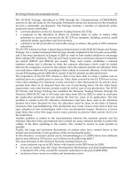
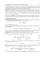
Response of the actuator to a step signal is shown Fig. 20 (a). As in section 3.2 concerning the
rotational link, the speed saturation is a consequence of the servovalve limited flow rate.
These results are interesting because even at the highest speed the presence of the passive
jack do not seem to seriously affect the performance of the system.
Fig. 20 (b) presents the force within the primary jack when operated with and without
passive jack. The reconstruction of the force was made according to the pressure values
within the chambers. The results are in agreement with the expectations: both dry and
viscous frictions are higher with the passive jack.
0 5 10 15 20 25 30 35 40 45 50
250
300
350
400
450
500
550
600
650
Time (s)
Position (mm)
Step response of the system with and without passive jac
k
Step response with passive jack
Step response without passive jack
Requested step signal
0 20 40 60 80 100 120 140 160 180 200
-4000
-3000
-2000
-1000
0
1000
2000
3000
4000
Force within the primary jack w/o the passive jack
Time (s)
Force (N)
Force with passive jack
Force without passive jack
Filtered force with passive jack (cut off frequency 10Hz)
Filtered force without passive jack (cut off frequency 10Hz)
(a) (b)
Fig. 20. Position step response (a) and force measured in the primary jack (b) with and
without passive jack
Asymmetry of the signal is due to the offset of the servovalve that has not been
compensated yet. Moreover the oscillations noted on this force signal are due to the poor
quality of the position measurement, which lead to a low quality control loop and speed
oscillations. These oscillations should be reduced by a better speed measurement but
creating an internal leak within the passive jack could also be another good option. Internal
leaks are acting as pressure dampers and would therefore naturally filter the force within
the primary jack.
As previously an identification of the system parameters has been performed to assess the
force feedback capabilities of the proposed system. The test bench was configured to be used
with and without the passive jack. The following table gives the values of all parameters in
both configurations.
As it could be expected viscous and dry friction are higher when the passive jack is mounted
on the bench. Due to its design itself (long guiding length, two concentric pipes sliding one
into each other) it is not surprising to see that most of the dry friction comes from the
passive jack. Viscous friction of the passive jack itself is not that high.
Parameter Test with passive jack Test without passive jack
Viscous friction N/(m/s) 24600 20600
Dry friction (N) 738 214
Offset (N) 305 -378
Table 4. Mechanical parameters issued from identification process
6. Conclusions
In this chapter we have tried to give the reader an overview of the studies currently carried
out at CEA LIST to make hydraulic manipulators work with demineralised water instead of
oil as a power fluid.
We showed that force and position performances of a Maestro elbow joint running with
water are globally similar or better than the performances of the one running with oil. Minor
design updates may be executed even if endurance tests proved that the joint is reliable up
Fromoiltopurewaterhydraulics,makingcleaner
andsaferforcefeedbackhighpayloadtelemanipulators 25
Fig. 19. Test rig
In the present design, the passive jack is one of the main components of the actuator. Due to
its design and location within the system’s kinematics it will act a damping system. It is
therefore interesting to test the performances of the system with and without this
component to characterize its influence on the whole behaviour.
Response of the actuator to a step signal is shown Fig. 20 (a). As in section 3.2 concerning the
rotational link, the speed saturation is a consequence of the servovalve limited flow rate.
These results are interesting because even at the highest speed the presence of the passive
jack do not seem to seriously affect the performance of the system.
Fig. 20 (b) presents the force within the primary jack when operated with and without
passive jack. The reconstruction of the force was made according to the pressure values
within the chambers. The results are in agreement with the expectations: both dry and
viscous frictions are higher with the passive jack.
0 5 10 15 20 25 30 35 40 45 50
250
300
350
400
450
500
550
600
650
Time (s)
Position (mm)
Step response of the system with and without passive jac
k
Step response with passive jack
Step response without passive jack
Requested step signal
0 20 40 60 80 100 120 140 160 180 200
-4000
-3000
-2000
-1000
0
1000
2000
3000
4000
Force within the primary jack w/o the passive jack
Time (s)
Force (N)
Force with passive jack
Force without passive jack
Filtered force with passive jack (cut off frequency 10Hz)
Filtered force without passive jack (cut off frequency 10Hz)
(a) (b)
Fig. 20. Position step response (a) and force measured in the primary jack (b) with and
without passive jack
Asymmetry of the signal is due to the offset of the servovalve that has not been
compensated yet. Moreover the oscillations noted on this force signal are due to the poor
quality of the position measurement, which lead to a low quality control loop and speed
oscillations. These oscillations should be reduced by a better speed measurement but
creating an internal leak within the passive jack could also be another good option. Internal
leaks are acting as pressure dampers and would therefore naturally filter the force within
the primary jack.
As previously an identification of the system parameters has been performed to assess the
force feedback capabilities of the proposed system. The test bench was configured to be used
with and without the passive jack. The following table gives the values of all parameters in
both configurations.
As it could be expected viscous and dry friction are higher when the passive jack is mounted
on the bench. Due to its design itself (long guiding length, two concentric pipes sliding one
into each other) it is not surprising to see that most of the dry friction comes from the
passive jack. Viscous friction of the passive jack itself is not that high.
Parameter Test with passive jack Test without passive jack
Viscous friction N/(m/s) 24600 20600
Dry friction (N) 738 214
Offset (N) 305 -378
Table 4. Mechanical parameters issued from identification process
6. Conclusions
In this chapter we have tried to give the reader an overview of the studies currently carried
out at CEA LIST to make hydraulic manipulators work with demineralised water instead of
oil as a power fluid.
We showed that force and position performances of a Maestro elbow joint running with
water are globally similar or better than the performances of the one running with oil. Minor
design updates may be executed even if endurance tests proved that the joint is reliable up
Robotics2010:CurrentandFutureChallenges26
to 500 hrs of operation without any observable degradation of its performance. Therefore it
seems clear that the Maestro actuator becomes a very good candidate for the design of a
complete water hydraulic manipulator.
Beside, pressure control water servovalve prototypes were tested with closed apertures and
connected to dead volumes for qualification and characterization with water. Although
most of the requirements are better or close to the expected values, the maximal pressure
difference between the two ports is lower than expected. A physical model was proposed in
order to identify which parameters could be responsible for this effect. Taking into account
that these tests are the first ones on the first prototype generation, these results are
encouraging and should foster developments in the area of water hydraulic servovalves.
At last the issue of integrating linear joint in serial architecture of hydraulic actuators has
been considered. Assessment of the performances required during standard operations
showed that creating a “pressure bus” within the manipulator to allow each servovalve to
obtain its required fluid flow was the best answer to the problem. An innovative design was
proposed. Preliminary tests on a functional mock-up have been presented and discussed.
In the next step, qualification of the water hydraulic joint equipped with a pressure
servovalve instead of the flow control pre-actuator will be made. This modification would
provide significant improvement of the force control loop in terms of accuracy, stability and
tuning procedures. Concerning the linear actuator performance of the position measurement
needs improvements to overcome limitations in the tuning of the control loop and provide a
speed signal compatible with force control requirements. It is proposed to investigate the
possibility to introduce data fusion procedures between two distinct sensors to reach the
requested quality level.
Then the integration of all these technologies to build an extended 6DOF water hydraulic
manipulator should be conceivable around 2010-2011.
7. Acknowledgements
This work, supported by the European Communities under the contract of association
between EURATOM and CEA, was carried out within the framework of the European
Fusion Development Agreement (EFDA). The views and opinions expressed herein do not
necessary reflect those of the European Commission.
8. References
Anderson, R.T. & Perry, L.Y. (2002). Mathematical Modeling of a Two Spool Flow Control
Servovalve Using a Pressure Control Pilot, Journal of Dynamic Systems, Measurement,
and Control, Vol. 124, Issue 3, September 2002, pp. 420-427.
Bidard, C.; Libersa, C.; Arhur, D.; Measson, Y.; Friconneau, J P. & Palmer, J. (2004).
Dynamic identification of the hydraulic MAESTRO manipulator – Relevance for
monitoring, Proceedings of SOFT23, Venice, 2004.
Dubus, G.; David, O.; Nozais, F.; Measson, Y.; Friconneau, J P. & Palmer, J. (2007).
Assessment of a water hydraulics joint for remote handling operations in the
divertor region, Proceedings of ISFNT8, Heidelberg, 2007.
Dubus, G.; David, O.; Nozais, F.; Measson, Y. & Friconneau, J P. (2008). Development of a
water hydraulics remote handling system for ITER maintenance, Proceedings of the
IARP/EURON Workshop on Robotics for Risky Interventions and Environmental
Surveillance, Benicàssim, 2008.
Eryilmaz, B. & Wilson, B.H. (2000). Combining leakage and orifice flows in a Hydraulic
Servovalve Model, ASME, 2000.
Gravez, P.; Leroux, C.; Irving, M.; Galbiati, L.; Raneda, A.; Siuko, M.; Maisonnier, D. &
Palmer, J. (2002). Model-based remote handling with the MAESTRO hydraulic
manipulator, Proceedings of SOFT22, Helsinki, 2002.
Guillon, M. (1992). Commande et asservissement hydrauliques et électrohydrauliques,
Lavoisier, Paris, 1992.
Kim, D.H. & Tsao, T C. (2000). A Linearized Electrohydraulic Servovalve Model for Valve
Dynamics Sensitivity Analysis and Control System Design, Journal of Dynamic
Systems, Measurement, and Control, Vol. 122, Issue 1, March 2000, pp. 179-187.
Li, P.Y. (2002). Dynamic Redesign of a Flow Control Servo-valve using a Pressure Control
Pilot, ASME Journal of Dynamic Systems, Measurement and Control, Vol. 124, No. 3,
Sept 2002.
Mattila, J.; Siuko, M.; Vilenius, M.; Muhammad, A.; Linna, O.; Sainio, A.; Mäkelä, A.;
Poutanen, J. & Saarinen, H. (2006). Development of water hydraulic manipulator,
Fusion Yearbook, Association Euratom-Tekes, Annual Report 2005, VTT Publications.
Measson, Y.; David, O.; Louveau, F. & Friconneau, J.P. (2003). Technology and control for
hydraulic manipulators, Fusion Engineering and Design, vol.69, September 2003.
Merrit, H. E. (1967). Hydraulic Control Systems, Wiley, New York, 1967.
Siuko, M.; Pitkäaho, M.; Raneda, A.; Poutanen, J.; Tammisto, J.; Palmer, J. & Vilenius, M.
(2003). Water hydraulic actuators for ITER maintenance devices, Fusion Engineering
and Design, Vol.69, September 2003.
Urata, E. & Yamashina C. (1998). Influence of flow force on the flapper of a water hydraulic
servovalve, JSME international journal. Series B, fluids and thermal
engineering, vol. 41, no2, 1998, pp. 278-285.
Fromoiltopurewaterhydraulics,makingcleaner
andsaferforcefeedbackhighpayloadtelemanipulators 27
to 500 hrs of operation without any observable degradation of its performance. Therefore it
seems clear that the Maestro actuator becomes a very good candidate for the design of a
complete water hydraulic manipulator.
Beside, pressure control water servovalve prototypes were tested with closed apertures and
connected to dead volumes for qualification and characterization with water. Although
most of the requirements are better or close to the expected values, the maximal pressure
difference between the two ports is lower than expected. A physical model was proposed in
order to identify which parameters could be responsible for this effect. Taking into account
that these tests are the first ones on the first prototype generation, these results are
encouraging and should foster developments in the area of water hydraulic servovalves.
At last the issue of integrating linear joint in serial architecture of hydraulic actuators has
been considered. Assessment of the performances required during standard operations
showed that creating a “pressure bus” within the manipulator to allow each servovalve to
obtain its required fluid flow was the best answer to the problem. An innovative design was
proposed. Preliminary tests on a functional mock-up have been presented and discussed.
In the next step, qualification of the water hydraulic joint equipped with a pressure
servovalve instead of the flow control pre-actuator will be made. This modification would
provide significant improvement of the force control loop in terms of accuracy, stability and
tuning procedures. Concerning the linear actuator performance of the position measurement
needs improvements to overcome limitations in the tuning of the control loop and provide a
speed signal compatible with force control requirements. It is proposed to investigate the
possibility to introduce data fusion procedures between two distinct sensors to reach the
requested quality level.
Then the integration of all these technologies to build an extended 6DOF water hydraulic
manipulator should be conceivable around 2010-2011.
7. Acknowledgements
This work, supported by the European Communities under the contract of association
between EURATOM and CEA, was carried out within the framework of the European
Fusion Development Agreement (EFDA). The views and opinions expressed herein do not
necessary reflect those of the European Commission.
8. References
Anderson, R.T. & Perry, L.Y. (2002). Mathematical Modeling of a Two Spool Flow Control
Servovalve Using a Pressure Control Pilot, Journal of Dynamic Systems, Measurement,
and Control, Vol. 124, Issue 3, September 2002, pp. 420-427.
Bidard, C.; Libersa, C.; Arhur, D.; Measson, Y.; Friconneau, J P. & Palmer, J. (2004).
Dynamic identification of the hydraulic MAESTRO manipulator – Relevance for
monitoring, Proceedings of SOFT23, Venice, 2004.
Dubus, G.; David, O.; Nozais, F.; Measson, Y.; Friconneau, J P. & Palmer, J. (2007).
Assessment of a water hydraulics joint for remote handling operations in the
divertor region, Proceedings of ISFNT8, Heidelberg, 2007.
Dubus, G.; David, O.; Nozais, F.; Measson, Y. & Friconneau, J P. (2008). Development of a
water hydraulics remote handling system for ITER maintenance, Proceedings of the
IARP/EURON Workshop on Robotics for Risky Interventions and Environmental
Surveillance, Benicàssim, 2008.
Eryilmaz, B. & Wilson, B.H. (2000). Combining leakage and orifice flows in a Hydraulic
Servovalve Model, ASME, 2000.
Gravez, P.; Leroux, C.; Irving, M.; Galbiati, L.; Raneda, A.; Siuko, M.; Maisonnier, D. &
Palmer, J. (2002). Model-based remote handling with the MAESTRO hydraulic
manipulator, Proceedings of SOFT22, Helsinki, 2002.
Guillon, M. (1992). Commande et asservissement hydrauliques et électrohydrauliques,
Lavoisier, Paris, 1992.
Kim, D.H. & Tsao, T C. (2000). A Linearized Electrohydraulic Servovalve Model for Valve
Dynamics Sensitivity Analysis and Control System Design, Journal of Dynamic
Systems, Measurement, and Control, Vol. 122, Issue 1, March 2000, pp. 179-187.
Li, P.Y. (2002). Dynamic Redesign of a Flow Control Servo-valve using a Pressure Control
Pilot, ASME Journal of Dynamic Systems, Measurement and Control, Vol. 124, No. 3,
Sept 2002.
Mattila, J.; Siuko, M.; Vilenius, M.; Muhammad, A.; Linna, O.; Sainio, A.; Mäkelä, A.;
Poutanen, J. & Saarinen, H. (2006). Development of water hydraulic manipulator,
Fusion Yearbook, Association Euratom-Tekes, Annual Report 2005, VTT Publications.
Measson, Y.; David, O.; Louveau, F. & Friconneau, J.P. (2003). Technology and control for
hydraulic manipulators, Fusion Engineering and Design, vol.69, September 2003.
Merrit, H. E. (1967). Hydraulic Control Systems, Wiley, New York, 1967.
Siuko, M.; Pitkäaho, M.; Raneda, A.; Poutanen, J.; Tammisto, J.; Palmer, J. & Vilenius, M.
(2003). Water hydraulic actuators for ITER maintenance devices, Fusion Engineering
and Design, Vol.69, September 2003.
Urata, E. & Yamashina C. (1998). Influence of flow force on the flapper of a water hydraulic
servovalve, JSME international journal. Series B, fluids and thermal
engineering, vol. 41, no2, 1998, pp. 278-285.
Robotics2010:CurrentandFutureChallenges28
OperationalSpaceDynamicsofaSpaceRobotandComputationalEfcientAlgorithm 29
Operational Space Dynamics of a Space Robot and Computational
EfcientAlgorithm
SatokoAbikoandGerdHirzinger
0
Operational Space Dynamics of a Space Robot
and Computational Efficient Algorithm
Satoko Abiko and Gerd Hirzinger
Institute of Robotics and Mechatronics,German Aerospace Center (DLR)
82334, Weßling, Germany
1. Introduction
On-orbit servicing space robot is one of the challenging applications in space robotic field.
Main task of the on-orbit space robot involves the tracking, the grasping and the positioning
of a target. The dynamics in operational space is useful to achieve such tasks in Cartesian
space. The operational space dynamics is a formulation of the dynamics of a complex branch-
ing redundant mechanism in task or operational points. Khatib proposed the formulation of a
serial robot manipulator system on ground in (Khatib, 1987). Russakow et. al. modified it for
a branching manipulator system in (Russakow et al., 1995). Chang and Khatib introduced effi-
cient algorithms for this formulation, especially for operational space inertia matrix in (Chang
& Khatib, 1999; 2000).
The operational space dynamics of the space robot is more complex than that of the ground-
based manipulator system since the base-satellite is inertially free. However, by virtue of no
fixed-base, the space robot is invertible in its modeling and arbitrary operational points to con-
trol can be chosen in a computational efficient manner. By making use of this unique character-
istic, we firstly propose an algorithm of the dynamics of a single operational point in the space
robot system. Then, by using the concept of the articulated-body algorithm(Featherstone,
1987), we propose a recursive computation of the dynamics of multi-operational points in the
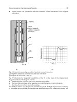
space robot. The numerical simulations are carried out using a two-arm space robot shown in
Fig. 1.
This chapter is organized as follows. Section 2 describes basic dynamic equations of free-
flying and free-floating space robots. Section 3 derives the operational space formulation of
both types of space robots. Section 4 briefly introduces spatial notation to represent complex
robot kinematics and dynamics, which is used for the derivation of the proposed algorithms.
Section 5 describes recursive algorithms of the generalized Jacobian matrix(Xu & Kanade,
1993), that is a Jacobian matrix including dynamical coupling between the base body and the
robot arm. Section 6 proposes computational efficient algorithms of the operational space
dynamics. Section 7 shows the simulation example of the proposed algorithms. Section 8
summarizes the conclusions.
2. Basic Equations
This section presents basic dynamic equations of the space robot. The main symbols used in
this section are defined in table 1.
2
Robotics2010:CurrentandFutureChallenges30
Fig. 1. Chaser-robot and target scenario
2.1 Linear and Angular Momentum Equations
The motion of the space robot is generally governed by the principle of the conservation of
momentum. When the spatial velocity of the base body, ˙x
b
= (v
T
b
, ω
T
b
)
T
∈ R
6×1
, and the
motion rate of the joints,
˙
φ
∈ R
n×1
, are considered as the generalized coordinates, total linear
and angular momentum,
M
0
∈ R
6×1
, are expressed as follows:
M
0
= H
b
˙x
b
+ H
bm
˙
φ . (1)
Note that
M
0
represents the total momentum around the center of mass of the base body.
In the absence of external forces, the total momentum is conserved. From eq. (1), the motion
of the base body is expressed by
˙
φ and
M
0
as:
˙x
b
= J
∗
b
˙
φ
+ H
−1
b
M
0
∈ R
6×1
, (2)
where
J
∗
b
= −H
−1
b
H
bm
∈ R
6×n
(3)
represents the generalized Jacobian matrix of the base body (Yokokohji et al., 1993). By in-
troducing the kinematic mapping of the i-th operational point, ˙x
e
i
= J
b
i
˙x
b
+ J
m
i
˙
φ, eq. (1)
provides the velocity of the operational point as follows:
˙x
e
i
= J
∗
m
i
˙
φ
+ J
b
i
H
−1
b
M
0
∈ R
6×1
, (4)
where
J
∗
m
i
= J
m
i
− J
b
i
H
−1
b
H
bm
∈ R
6×n
(5)
is called the generalized Jacobian matrix of the operational point (Umetani & Yoshida, 1989).
The above generalized Jacobian matrix, (5), is for the case that a single point is selected as an
operational point. This matrix is simply extended to the case of the multi-operational points
n : number of joints
p : number of operational points
˙x
b
∈ R
6×1
: linear and angular velocity of the base.
˙
φ
∈ R
n×1
: motion rate of the arms.
˙x
e
=
˙x
e
1
.
.
.
˙x
e
p
∈ R
6p×1
: linear and angular velocity of the operational points (i =
1 ···p).
H
b
∈ R
6×6
: inertia matrix of the base.
H
m
∈ R
n×n
: inertia matrix of the arms.
H
bm
∈ R
6×n
: coupling inertia matrix between the base and the arms.
c
b
∈ R
6×1
: non-linear velocity dependent term of the base.
c
m
∈ R
n×1
: non-linear velocity dependent term of the arms.
F
b
∈ R
6×1
: force and moment exerted on the base.
F
e
∈ R
6p×1
: force and moment exerted on the operational points.
τ
∈ R
n×1
: torque on joints.
J
b
i
∈ R
6×6
: Jacobian matrix of the base in terms of the i-th operational
point.
J
m
i
∈ R
6×n
: Jacobian matrix of the arms in terms of the i-th operational
point.
J
∗
b
∈ R
6×6
: Generalized Jacobian matrix of the base body.
J
∗
m
i
∈ R
6×n
: Generalized Jacobian matrix of the arms in terms of the
i-th operational point.
Table 1. Main Notation
by augmenting the Jacobian matrix of each operational point. In section 5, we derive recursive
calculations of the matrices, (3) and (5).
2.2 Equations of Motion
The general dynamic equation of the space robot is described by the following expression (Xu
& Kanade, 1993):
H
b
H
bm
H
T
bm
H
m
¨x
b
¨
φ
+
c
b
c
m
=
F
b
τ
+
J
T
b
J
T
m
F
e
. (6)
where ˙x
b
= (v
T
b
, ω
T
b
)
T
∈ R
6×1
, and the motion rate of the joints,
˙
φ ∈ R
n×1
are considered
as the generalized coordinates. When
F
b
is actively generated (e.g. jet thrusters or reaction
wheels etc.), the system is called a free-flying robot. If no active actuators are applied on the
OperationalSpaceDynamicsofaSpaceRobotandComputationalEfcientAlgorithm 31
Fig. 1. Chaser-robot and target scenario
2.1 Linear and Angular Momentum Equations
The motion of the space robot is generally governed by the principle of the conservation of
momentum. When the spatial velocity of the base body, ˙x
b
= (v
T
b
, ω
T
b
)
T
∈ R
6×1
, and the
motion rate of the joints,
˙
φ
∈ R
n×1
, are considered as the generalized coordinates, total linear
and angular momentum,
M
0
∈ R
6×1
, are expressed as follows:
M
0
= H
b
˙x
b
+ H
bm
˙
φ . (1)
Note that
M
0
represents the total momentum around the center of mass of the base body.
In the absence of external forces, the total momentum is conserved. From eq. (1), the motion
of the base body is expressed by
˙
φ and
M
0
as:
˙x
b
= J
∗
b
˙
φ
+ H
−1
b
M
0
∈ R
6×1
, (2)
where
J
∗
b
= −H
−1
b
H
bm
∈ R
6×n
(3)
represents the generalized Jacobian matrix of the base body (Yokokohji et al., 1993). By in-
troducing the kinematic mapping of the i-th operational point, ˙x
e
i
= J
b
i
˙x
b
+ J
m
i
˙
φ, eq. (1)
provides the velocity of the operational point as follows:
˙x
e
i
= J
∗
m
i
˙
φ
+ J
b
i
H
−1
b
M
0
∈ R
6×1
, (4)
where
J
∗
m
i
= J
m
i
− J
b
i
H
−1
b
H
bm
∈ R
6×n
(5)
is called the generalized Jacobian matrix of the operational point (Umetani & Yoshida, 1989).
The above generalized Jacobian matrix, (5), is for the case that a single point is selected as an
operational point. This matrix is simply extended to the case of the multi-operational points
n : number of joints
p : number of operational points
˙x
b
∈ R
6×1
: linear and angular velocity of the base.
˙
φ
∈ R
n×1
: motion rate of the arms.
˙x
e
=
˙x
e
1
.
.
.
˙x
e
p
∈ R
6p×1
: linear and angular velocity of the operational points (i =
1 ···p).
H
b
∈ R
6×6
: inertia matrix of the base.
H
m
∈ R
n×n
: inertia matrix of the arms.
H
bm
∈ R
6×n
: coupling inertia matrix between the base and the arms.
c
b
∈ R
6×1
: non-linear velocity dependent term of the base.
c
m
∈ R
n×1
: non-linear velocity dependent term of the arms.
F
b
∈ R
6×1
: force and moment exerted on the base.
F
e
∈ R
6p×1
: force and moment exerted on the operational points.
τ
∈ R
n×1
: torque on joints.
J
b
i
∈ R
6×6
: Jacobian matrix of the base in terms of the i-th operational
point.
J
m
i
∈ R
6×n
: Jacobian matrix of the arms in terms of the i-th operational
point.
J
∗
b
∈ R
6×6
: Generalized Jacobian matrix of the base body.
J
∗
m
i
∈ R
6×n
: Generalized Jacobian matrix of the arms in terms of the
i-th operational point.
Table 1. Main Notation
by augmenting the Jacobian matrix of each operational point. In section 5, we derive recursive
calculations of the matrices, (3) and (5).
2.2 Equations of Motion
The general dynamic equation of the space robot is described by the following expression (Xu
& Kanade, 1993):
H
b
H
bm
H
T
bm
H
m
¨x
b
¨
φ
+
c
b
c
m
=
F
b
τ
+
J
T
b
J
T
m
F
e
. (6)
where ˙x
b
= (v
T
b
, ω
T
b
)
T
∈ R
6×1
, and the motion rate of the joints,
˙
φ ∈ R
n×1
are considered
as the generalized coordinates. When
F
b
is actively generated (e.g. jet thrusters or reaction
wheels etc.), the system is called a free-flying robot. If no active actuators are applied on the
Robotics2010:CurrentandFutureChallenges32
base, the system is termed a free-floating robot. The integral of the upper part of eq. (6) de-
scribes the total linear and angular momentum around the center of mass of the base body
and corresponds to the equation (1).
2.3 Dynamics of a Free-Floating Space Robot
The dynamic equation of the free-floating space robot can be furthermore reduced a form
expressed with only joint acceleration,
¨
φ, by eliminating the base body acceleration, ¨x
b
, from
eq. (6):
H
∗
m
¨
φ
+ c
∗
m
= τ + J
∗T
b
F
b
+ J
∗T
m
F
e
(7)
where H
∗
m
= H
m
− H
T
bm
H
−1
b
H
bm
∈ R
n×n
and c
∗
m
= c
m
− H
T
bm
H
−1
b
c
b
∈ R
n×1
represent
generalized inertia matrix and generalized non-linear velocity dependent term, respectively.
3. Operational Space Formulation
The operational space dynamics is useful to control the system in the operational space, which
represents the dynamics projected from the joint space to the operational space. The two types
of space robot dynamics are described in the following subsections. One is for the free-flying
space robot and the other is for the free-floating space robot. This section derives the equations
of motion for the space robots consisting of n-links with p operational points.
3.1 Free-Flying Space Robot
The operational space dynamics of the free-flying space robot is described in the following
form:
Γ
e
¨x
e
+ µ
e
= F
in
e
+ F
e
, (8)
where
F
b
τ
= J
T
e
F
in
e
.
F
e
∈ R
6p×1
consists of the 6 × 1 external force of each of p operational points. J
e
∈
R
6p×(6+(n−1))
consists of Jacobian matrix of each operational point.
F
e
=
F
e
1
.
.
.
F
e
p
and J
e
=
J
b
1
, J
m
1
.
.
.
.
.
.
J
b
p
, J
m
p
.
The operational space inertia matrix of the free-flying space robot, Γ
e
, is an 6p ×6p symmetric
positive definite matrix. Its inverse matrix can be expressed as :
Γ
−1
e
= J
e
H
−1
J
T
e
, H =
H
b
H
bm
H
T
bm
H
m
. (9)
The operational space centrifugal and Coriolis forces, µ
e
, is expressed as :
µ
e
= J
T+
e
c
b
c
m
−Γ
e
d
dt
J
e
˙x
b
˙
φ
, (10)
where J
+
e
is the dynamically consistent generalized inverse of the Jacobian matrix J
e
for the
free-flying space robot to minimize the instantaneous kinetic energy of the space robot:
J
+
e
= H
−1
J
T
e
Γ
e
. (11)
Fig. 2. Notation Representation
3.2 Free-Floating Space Robot
In the free-floating space robot, no active forces exist on the base (e.g. F
b
= 0). Then, the
system can be described as the reduced form in the joint space by using eq. (7). Its operational
space dynamics can be derived from eqs. (5) and (7):
Γ
e
¨x
e
+ Γ
e
µ = Γ
e
Λ
−1
J
∗T+
m
τ + F
e
, (12)
where
Γ
−1
e
= Λ
−1
+ Λ
−1
b
∈ R
6p×6p
,
Λ
−1
= J
∗
m
H
∗−1
m
J
∗T
m
, Λ
−1
b
= J
b
H
−1
b
J
T
b
.
The matrix,
(Λ
−1
+ Λ
−1
b
), corresponds to the inertia matrix described in eq. (9). The vector, µ,
expresses the bias acceleration vector resulting from the Coriolis and centrifugal forces as:
µ
= Λ
−1
J
∗+
m
c
∗
m
−
˙
J
∗
m
˙
φ
−
d
dt
(J
b
H
−1
b
)M
0
∈ R
6p×1
.
where
J
∗+
m
= H
∗−1
m
J
∗T
m
Λ (13)
represents the dynamically consistent generalized inverse of the Jacobian matrix J
∗
m
for the
free-floating space robot. Compared with eq. (8), the relationship Γ
e
µ = µ
e
is obtained. Note
that each dynamic equation described in this section is expressed in the inertial frame. Section
6 describes the efficient algorithms for the operational space dynamics represented in this
section.
4. Spatial Notation
The Spatial Notation is well-known and intuitive notation in modeling kinematics and dynam-
ics of articulated robot systems, introduced by Featherstone (Featherstone (1987); Chang &
Khatib (1999)). This section concisely reviews the basic spatial notation. The main symbols
used in the spatial notation are defined in Table 2. The symbols are expressed in the frame
fixed at each link. (See. Fig. 2).
OperationalSpaceDynamicsofaSpaceRobotandComputationalEfcientAlgorithm 33
base, the system is termed a free-floating robot. The integral of the upper part of eq. (6) de-
scribes the total linear and angular momentum around the center of mass of the base body
and corresponds to the equation (1).
2.3 Dynamics of a Free-Floating Space Robot
The dynamic equation of the free-floating space robot can be furthermore reduced a form
expressed with only joint acceleration,
¨
φ, by eliminating the base body acceleration, ¨x
b
, from
eq. (6):
H
∗
m
¨
φ
+ c
∗
m
= τ + J
∗T
b
F
b
+ J
∗T
m
F
e
(7)
where H
∗
m
= H
m
− H
T
bm
H
−1
b
H
bm
∈ R
n×n
and c
∗
m
= c
m
− H
T
bm
H
−1
b
c
b
∈ R
n×1
represent
generalized inertia matrix and generalized non-linear velocity dependent term, respectively.
3. Operational Space Formulation
The operational space dynamics is useful to control the system in the operational space, which
represents the dynamics projected from the joint space to the operational space. The two types
of space robot dynamics are described in the following subsections. One is for the free-flying
space robot and the other is for the free-floating space robot. This section derives the equations
of motion for the space robots consisting of n-links with p operational points.
3.1 Free-Flying Space Robot
The operational space dynamics of the free-flying space robot is described in the following
form:
Γ
e
¨x
e
+ µ
e
= F
in
e
+ F
e
, (8)
where
F
b
τ
= J
T
e
F
in
e
.
F
e
∈ R
6p×1
consists of the 6 × 1 external force of each of p operational points. J
e
∈
R
6p×(6+(n−1))
consists of Jacobian matrix of each operational point.
F
e
=
F
e
1
.
.
.
F
e
p
and J
e
=
J
b
1
, J
m
1
.
.
.
.
.
.
J
b
p
, J
m
p
.
The operational space inertia matrix of the free-flying space robot, Γ
e
, is an 6p ×6p symmetric
positive definite matrix. Its inverse matrix can be expressed as :
Γ
−1
e
= J
e
H
−1
J
T
e
, H =
H
b
H
bm
H
T
bm
H
m
. (9)
The operational space centrifugal and Coriolis forces, µ
e
, is expressed as :
µ
e
= J
T+
e
c
b
c
m
−Γ
e
d
dt
J
e
˙x
b
˙
φ
, (10)
where J
+
e
is the dynamically consistent generalized inverse of the Jacobian matrix J
e
for the
free-flying space robot to minimize the instantaneous kinetic energy of the space robot:
J
+
e
= H
−1
J
T
e
Γ
e
. (11)
Fig. 2. Notation Representation
3.2 Free-Floating Space Robot
In the free-floating space robot, no active forces exist on the base (e.g. F
b
= 0). Then, the
system can be described as the reduced form in the joint space by using eq. (7). Its operational
space dynamics can be derived from eqs. (5) and (7):
Γ
e
¨x
e
+ Γ
e
µ = Γ
e
Λ
−1
J
∗T+
m
τ + F
e
, (12)
where
Γ
−1
e
= Λ
−1
+ Λ
−1
b
∈ R
6p×6p
,
Λ
−1
= J
∗
m
H
∗−1
m
J
∗T
m
, Λ
−1
b
= J
b
H
−1
b
J
T
b
.
The matrix,
(Λ
−1
+ Λ
−1
b
), corresponds to the inertia matrix described in eq. (9). The vector, µ,
expresses the bias acceleration vector resulting from the Coriolis and centrifugal forces as:
µ
= Λ
−1
J
∗+
m
c
∗
m
−
˙
J
∗
m
˙
φ
−
d
dt
(J
b
H
−1
b
)M
0
∈ R
6p×1
.
where
J
∗+
m
= H
∗−1
m
J
∗T
m
Λ (13)
represents the dynamically consistent generalized inverse of the Jacobian matrix J
∗
m
for the
free-floating space robot. Compared with eq. (8), the relationship Γ
e
µ = µ
e
is obtained. Note
that each dynamic equation described in this section is expressed in the inertial frame. Section
6 describes the efficient algorithms for the operational space dynamics represented in this
section.
4. Spatial Notation
The Spatial Notation is well-known and intuitive notation in modeling kinematics and dynam-
ics of articulated robot systems, introduced by Featherstone (Featherstone (1987); Chang &
Khatib (1999)). This section concisely reviews the basic spatial notation. The main symbols
used in the spatial notation are defined in Table 2. The symbols are expressed in the frame
fixed at each link. (See. Fig. 2).
Robotics2010:CurrentandFutureChallenges34
v
i
∈ R
6×1
: spatial velocity of link i.
a
i
∈ R
6×1
: spatial acceleration of link i.
f
i
∈ R
6×1
: composite force of link i.
f
∗
i
∈ R
6×1
: spatial force of link i.
L
i
∈ R
6×1
: composite momentum of link i.
L
∗
i
∈ R
6×1
: spatial momentum of link i.
I
C
i
∈ R
6×1
: composite inertia matrix of link i.
Table 2. Main Symbols in Spatial Notation
4.1 Spatial Notation
In the spatial notation, linear and angular components are dealt with in a unified framework
and results in a concise form ( e.g. 6
×1 vector or 6 ×6 matrix ). In this expression, a spatial
velocity, v
i
, and a spatial force, f
i
, of link i are defined as :
v
i
=
v
i
ω
i
and f
i
=
F
i
T
i
,
where v
i
, ω
i
, F
i
, and T
i
represent the 3 ×1 linear and angular velocity, the force and moment
in terms of link i in frame i, respectively.
The simple joint model, S
i
∈ R
6×1
, for prismatic and rotational joint is defined, so that 1 is
assigned along the prismatic or rotational axis : e.g.
S
i
=
[
0 0 1 0 0 0
]
T
for prismatic joint at z axis
and
S
i
=
[
0 0 0 0 0 1
]
T
for rotational joint at z axis.
More complex multi-degrees-of-freedom joint is introduced in (Featherstone, 1987; Lilly,
1992).
The spatial inertia matrix of link i in frame c
i
, I
c
i
, is a symmetric positive definite matrix as:
I
c
i
=
m
i
E
3
0
0 I
c
i
∈ R
6×6
,
where m
i
is the mass of link i, and I
c
i
∈ R
3×3
is the inertia matrix around the center of mass
of the link i in frame c
i
. E
3
stands for the 3 ×3 identity matrix.
The 6
× 6 spatial transformation matrix,
h
i
X, transforms a spatial quantity from frame i to
frame h as:
h
i
X =
h
i
R 0
h
r
i
h
i
R
h
i
R
∈ R
6×6
. (14)
where
h
i
R ∈ R
3×3
is a rotation matrix and
h
r
i
∈ R
3×1
is a position vector from the origin of
frame h to that of frame i expressed in frame h.
{·}denotes the skew-symmetric matrix. Unlike
Σ
i
Σ
b
Σ
e
Link 0
( Base body )
Link 1
Link n
F
e
Link 2
φ
1
φ
2
φ
n
( Operational Point )
Fig. 3. Forward Chain Approach
Σ
i
Σ
b
Σ
e
Link 0
( Base body )
Link 1
Link n
F
e
Link 2
φ
1
φ
2
φ
n
( Operational Point )
Fig. 4. Inverted Chain Approach
the conventional 3
×3 rotational matrix, the spatial transformation matrix is not orthogonal.
The transformation matrix from frame h to frame i,
i
h
X, is expressed as:
i
h
X =
h
i
R
T
0
h
r
i
h
i
R
T
h
i
R
T
∈ R
6×6
. (15)
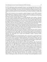
4.2 Spatial Quantity
The most of the spatial quantities including the spatial velocity, acceleration, and the spatial
force are iteratively calculated. To carry out the iterative calculation, two approaches can be
found, which are dependent on the direction of the iteration. In the first approach, the kine-
matic quantities such as the velocity and the acceleration are computed by outward recursion
from the link 0 toward the operational points as shown in Fig. 3 and the spatial force is ob-
tained by inward recursion from the operational points toward the link 0. This approach is
termed forward chain approach. In the second approach, the direction of the recursive calcu-
lation is opposed to the first one, so that the kinematic quantities are computed by inward
recursion and the spatial force is obtained by outward recursion as shown in Fig. 4. This
approach is termed inverted chain approach.
4.2.1 Forward Chain Approach
In the forward chain approach, the spatial velocity of link i is computed by the spatial velocity
of its parent link and its joint velocity as:
v
i
=
h
i
X
T
v
h
+ S
i
˙
φ
i
, (v
i
= v
0
at i = 0) . (16)
The spatial acceleration can be calculated similarly in the following form:
a
i
=
h
i
X
T
a
h
+ v
i
×S
i
˙
φ
i
+ S
i
¨
φ
i
, (a
i
= a
0
at i = 0) . (17)
where
× denotes the spatial cross-product operator associated with a spatial vector
a
T
, b
T
T
defined as:
a
b
× =
b a
0
b
∈ R
6×6
.
OperationalSpaceDynamicsofaSpaceRobotandComputationalEfcientAlgorithm 35
v
i
∈ R
6×1
: spatial velocity of link i.
a
i
∈ R
6×1
: spatial acceleration of link i.
f
i
∈ R
6×1
: composite force of link i.
f
∗
i
∈ R
6×1
: spatial force of link i.
L
i
∈ R
6×1
: composite momentum of link i.
L
∗
i
∈ R
6×1
: spatial momentum of link i.
I
C
i
∈ R
6×1
: composite inertia matrix of link i.
Table 2. Main Symbols in Spatial Notation
4.1 Spatial Notation
In the spatial notation, linear and angular components are dealt with in a unified framework
and results in a concise form ( e.g. 6
×1 vector or 6 ×6 matrix ). In this expression, a spatial
velocity, v
i
, and a spatial force, f
i
, of link i are defined as :
v
i
=
v
i
ω
i
and f
i
=
F
i
T
i
,
where v
i
, ω
i
, F
i
, and T
i
represent the 3 ×1 linear and angular velocity, the force and moment
in terms of link i in frame i, respectively.
The simple joint model, S
i
∈ R
6×1
, for prismatic and rotational joint is defined, so that 1 is
assigned along the prismatic or rotational axis : e.g.
S
i
=
[
0 0 1 0 0 0
]
T
for prismatic joint at z axis
and
S
i
=
[
0 0 0 0 0 1
]
T
for rotational joint at z axis.
More complex multi-degrees-of-freedom joint is introduced in (Featherstone, 1987; Lilly,
1992).
The spatial inertia matrix of link i in frame c
i
, I
c
i
, is a symmetric positive definite matrix as:
I
c
i
=
m
i
E
3
0
0 I
c
i
∈ R
6×6
,
where m
i
is the mass of link i, and I
c
i
∈ R
3×3
is the inertia matrix around the center of mass
of the link i in frame c
i
. E
3
stands for the 3 ×3 identity matrix.
The 6
× 6 spatial transformation matrix,
h
i
X, transforms a spatial quantity from frame i to
frame h as:
h
i
X =
h
i
R 0
h
r
i
h
i
R
h
i
R
∈ R
6×6
. (14)
where
h
i
R ∈ R
3×3
is a rotation matrix and
h
r
i
∈ R
3×1
is a position vector from the origin of
frame h to that of frame i expressed in frame h.
{·}denotes the skew-symmetric matrix. Unlike
Σ
i
Σ
b
Σ
e
Link 0
( Base body )
Link 1
Link n
F
e
Link 2
φ
1
φ
2
φ
n
( Operational Point )
Fig. 3. Forward Chain Approach
Σ
i
Σ
b
Σ
e
Link 0
( Base body )
Link 1
Link n
F
e
Link 2
φ
1
φ
2
φ
n
( Operational Point )
Fig. 4. Inverted Chain Approach
the conventional 3
×3 rotational matrix, the spatial transformation matrix is not orthogonal.
The transformation matrix from frame h to frame i,
i
h
X, is expressed as:
i
h
X =
h
i
R
T
0
h
r
i
h
i
R
T
h
i
R
T
∈ R
6×6
. (15)
4.2 Spatial Quantity
The most of the spatial quantities including the spatial velocity, acceleration, and the spatial
force are iteratively calculated. To carry out the iterative calculation, two approaches can be
found, which are dependent on the direction of the iteration. In the first approach, the kine-
matic quantities such as the velocity and the acceleration are computed by outward recursion
from the link 0 toward the operational points as shown in Fig. 3 and the spatial force is ob-
tained by inward recursion from the operational points toward the link 0. This approach is
termed forward chain approach. In the second approach, the direction of the recursive calcu-
lation is opposed to the first one, so that the kinematic quantities are computed by inward
recursion and the spatial force is obtained by outward recursion as shown in Fig. 4. This
approach is termed inverted chain approach.
4.2.1 Forward Chain Approach
In the forward chain approach, the spatial velocity of link i is computed by the spatial velocity
of its parent link and its joint velocity as:
v
i
=
h
i
X
T
v
h
+ S
i
˙
φ
i
, (v
i
= v
0
at i = 0) . (16)
The spatial acceleration can be calculated similarly in the following form:
a
i
=
h
i
X
T
a
h
+ v
i
×S
i
˙
φ
i
+ S
i
¨
φ
i
, (a
i
= a
0
at i = 0) . (17)
where
× denotes the spatial cross-product operator associated with a spatial vector
a
T
, b
T
T
defined as:
a
b
× =
b a
0
b
∈ R
6×6
.
Robotics2010:CurrentandFutureChallenges36
The iterative calculation of the composite force acted on the link h is defined as:
f
h
= f
∗
h
+
h
i
X f
i
, ( f
n
= f
∗
n
) , (18)
where
f
∗
i
= I
i
a
i
+ v
i
×I
i
v
i
. (19)
I
i
is the spatial inertia matrix of link i in frame i expressed as:
I
i
=
i
c
i
X I
c
i
i
c
i
X
T
,
where I
i
is a symmetric positive definite matrix. The integral of eq. (19) represents the spatial
momentum of link h and the composite momentum of link h can be derived as :
L
h
= I
h
v
h
+
h
i
XL
i
, (L
n
= I
n
v
n
) . (20)
In the above recursive calculation of the momentum, the composite rigid-body inertia of link
h can be obtained as follows, which is the summation of inertia matrices of link h and its
children links (Lilly, 1992):
I
C
h
= I
h
+
h
i
X I
C
i
h
i
X
T
, (I
C
n
= I
n
) . (21)
Note that the velocity and the acceleration of link 0 are arbitrary, not only zero but also non-
zero values are acceptable since our main focus is on the free-flying or free-floating space
robots. We assume that those values are measurable or can be estimated.
4.2.2 Inverted Chain Approach
In the inverted chain approach, the transformation matrix,
i
h
X, is used to obtain each spatial
quantity. As mentioned before, the direction to calculate each quantity is opposed to that of
the forward chain approach.
The spatial velocity is expressed as:
v
h
=
i
h
X
T
(
v
i
−S
i
˙
φ
i
)
, (v
h
= v
n
at h = n) . (22)
The spatial acceleration is described as:
a
h
=
i
h
X
T
a
i
−v
i
×S
i
˙
φ
i
−S
i
¨
φ
i
,
(a
h
= a
n
at h = n) . (23)
The composite force is derived as:
f
i
= f
∗
i
+
i
h
X f
h
, ( f
0
= f
∗
0
) . (24)
Under the same conditions, the results of the forward chain approach and the inverted chain
approach are consistent.
5. Recursive Computation of Generalized Jacobian Matrix
This section presents efficient recursive calculations of the generalized Jacobian matrices in-
troduced in (3) and (5). We introduce here the recursive algorithms in the framework of the
spatial notation. Yokokohji proposed the recursive calculation of the generalized Jacobian
matrix in (Yokokohji et al., 1993). However, by using the spatial notation, the recursive calcu-
lations can be improved to simpler and faster methods than one proposed in (Yokokohji et al.,
1993).
5.1 Generalized Jacobian Matrix of Base Body (Link 0)
In the recursive expression, the total linear and angular momentum around the origin of frame
0 is expressed from eqs. (16) and (20) as follows :
L
0
=
n
∑
k=0
0
k
X I
k
v
k
= I
0
v
0
+
n
∑
k=1
0
k
X I
k
0
k
X
T
v
0
+ S
k
˙
φ
k
. (25)
where
M
0
=
I
0
XL
0
. From eq. (25), the velocity of the base can be expressed as a function of
the velocity of the joint as :
v
0
= −
I
C
0
−1
n
∑
k=1
0
k
X I
C
k
S
k
˙
φ
k
+
I
C
0
−1
L
0
, (26)
where I
C
0
and I
C
k
denote composite rigid-body inertia matrix of the base and for link k com-
puted by (21), respectively. The coefficient of the first term on the righthand side corresponds
to the generalized Jacobian matrix of the base (link 0) in the frame 0 :
0
J
∗
b
= −
I
C
0
−1
∑
k
0
k
X
T
I
C
k
S
k
. (27)
Transformed into the inertial frame, eq. (27) equals to the expression (3) :
J
∗
b
=
I
0
X
0
J
∗
b
. (28)
5.2 Generalized Jacobian Matrix of Operational Point
Once
0
J
∗
b
is obtained, the generalized Jacobian matrix of the operational point is straightfor-
wardly derived. The spatial velocity of the operational point e
i
can be expressed as:
v
e
i
=
n
e
i
X
T
v
n
, (29)
where v
n
is the velocity of the link n, on which the operational point is determined, and is
obtained from eq. (16). By substituting (26) into (29), the generalized Jacobian matrix of the
operational point in the frame e
i
can be derived as:
e
i
J
∗
m
i
=
n
∑
k=1
k
e
i
X
T
S
k
−
0
e
i
X
T
I
C
0
−1
I
C
k
S
k
(30)
Consequently, the generalized Jacobian matrix in the inertial frame, (5), can be obtained as
follows:
J
∗
m
i
=
I
e
i
X
e
i
J
∗
m
i
. (31)
OperationalSpaceDynamicsofaSpaceRobotandComputationalEfcientAlgorithm 37
The iterative calculation of the composite force acted on the link h is defined as:
f
h
= f
∗
h
+
h
i
X f
i
, ( f
n
= f
∗
n
) , (18)
where
f
∗
i
= I
i
a
i
+ v
i
×I
i
v
i
. (19)
I
i
is the spatial inertia matrix of link i in frame i expressed as:
I
i
=
i
c
i
X I
c
i
i
c
i
X
T
,
where I
i
is a symmetric positive definite matrix. The integral of eq. (19) represents the spatial
momentum of link h and the composite momentum of link h can be derived as :
L
h
= I
h
v
h
+
h
i
XL
i
, (L
n
= I
n
v
n
) . (20)
In the above recursive calculation of the momentum, the composite rigid-body inertia of link
h can be obtained as follows, which is the summation of inertia matrices of link h and its
children links (Lilly, 1992):
I
C
h
= I
h
+
h
i
X I
C
i
h
i
X
T
, (I
C
n
= I
n
) . (21)
Note that the velocity and the acceleration of link 0 are arbitrary, not only zero but also non-
zero values are acceptable since our main focus is on the free-flying or free-floating space
robots. We assume that those values are measurable or can be estimated.
4.2.2 Inverted Chain Approach
In the inverted chain approach, the transformation matrix,
i
h
X, is used to obtain each spatial
quantity. As mentioned before, the direction to calculate each quantity is opposed to that of
the forward chain approach.
The spatial velocity is expressed as:
v
h
=
i
h
X
T
(
v
i
−S
i
˙
φ
i
)
, (v
h
= v
n
at h = n) . (22)
The spatial acceleration is described as:
a
h
=
i
h
X
T
a
i
−v
i
×S
i
˙
φ
i
−S
i
¨
φ
i
,
(a
h
= a
n
at h = n) . (23)
The composite force is derived as:
f
i
= f
∗
i
+
i
h
X f
h
, ( f
0
= f
∗
0
) . (24)
Under the same conditions, the results of the forward chain approach and the inverted chain
approach are consistent.
5. Recursive Computation of Generalized Jacobian Matrix
This section presents efficient recursive calculations of the generalized Jacobian matrices in-
troduced in (3) and (5). We introduce here the recursive algorithms in the framework of the
spatial notation. Yokokohji proposed the recursive calculation of the generalized Jacobian
matrix in (Yokokohji et al., 1993). However, by using the spatial notation, the recursive calcu-
lations can be improved to simpler and faster methods than one proposed in (Yokokohji et al.,
1993).
5.1 Generalized Jacobian Matrix of Base Body (Link 0)
In the recursive expression, the total linear and angular momentum around the origin of frame
0 is expressed from eqs. (16) and (20) as follows :
L
0
=
n
∑
k=0
0
k
X I
k
v
k
= I
0
v
0
+
n
∑
k=1
0
k
X I
k
0
k
X
T
v
0
+ S
k
˙
φ
k
. (25)
where
M
0
=
I
0
XL
0
. From eq. (25), the velocity of the base can be expressed as a function of
the velocity of the joint as :
v
0
= −
I
C
0
−1
n
∑
k=1
0
k
X I
C
k
S
k
˙
φ
k
+
I
C
0
−1
L
0
, (26)
where I
C
0
and I
C
k
denote composite rigid-body inertia matrix of the base and for link k com-
puted by (21), respectively. The coefficient of the first term on the righthand side corresponds
to the generalized Jacobian matrix of the base (link 0) in the frame 0 :
0
J
∗
b
= −
I
C
0
−1
∑
k
0
k
X
T
I
C
k
S
k
. (27)
Transformed into the inertial frame, eq. (27) equals to the expression (3) :
J
∗
b
=
I
0
X
0
J
∗
b
. (28)
5.2 Generalized Jacobian Matrix of Operational Point
Once
0
J
∗
b
is obtained, the generalized Jacobian matrix of the operational point is straightfor-
wardly derived. The spatial velocity of the operational point e
i
can be expressed as:
v
e
i
=
n
e
i
X
T
v
n
, (29)
where v
n
is the velocity of the link n, on which the operational point is determined, and is
obtained from eq. (16). By substituting (26) into (29), the generalized Jacobian matrix of the
operational point in the frame e
i
can be derived as:
e
i
J
∗
m
i
=
n
∑
k=1
k
e
i
X
T
S
k
−
0
e
i
X
T
I
C
0
−1
I
C
k
S
k
(30)
Consequently, the generalized Jacobian matrix in the inertial frame, (5), can be obtained as
follows:
J
∗
m
i
=
I
e
i
X
e
i
J
∗
m
i
. (31)
Robotics2010:CurrentandFutureChallenges38
6. Efficient Algorithms of Operational Space Dynamics
This section describes recursive algorithms of the operational space dynamics, eq. (8). We
recall here the operational space dynamics :
Γ
e
¨x
e
+ µ
e
= F
e
,
F
b
τ
= J
T
e
F
e
. (32)
A main focus is on developing computational efficient algorithms of Γ
e
and µ
e
of a n-link,
p-operational-point branching space robot system. The derivation of J
e
is omitted in this
chapter since its algorithm is well-known. The algorithms of Γ
e
and µ
e
are developed with
the concept of the articulated body dynamics (Featherstone, 1987; Lilly, 1992). Firstly, the
operational space formulation of a single operational point on the space robot is developed
by using the inverted chain approach. Then, the algorithms of the multi-operational point
system are further developed.
6.1 Single Operational Point in Space Robot
As mentioned in Section 1, a unique characteristic of the space robot is that the base satellite is
inertially free and the system is invertible in its modeling unlike the ground-based robot sys-
tem. Based on this characteristic, the operational space dynamics of the space robot is derived
in the framework of the articulated-body dynamics. In the conventional articulated-body dy-
namics, the articulated-body inertia and its associated bias force are calculated inward from
the operational point to the base body (link 0). When the system is inverted, the articulated-
body dynamics is calculated in the opposed direction, namely outward from the base body
to the operational point. This approach introduced as the inertia propagation method in (Lilly,
1992). We make use of the inverted chain approach for the iterative calculation of the inertia
matrix, Γ
e
, and the bias force vector, µ
e
in the operational space.
6.1.1 Operational space inertia matrix
Operational space inertia matrix corresponds to the articulated-body inertia calculated from
the base body to the operational point with the initial condition, I
A
0
= I
0
:
I
A
i
= I
i
+
i
I
A
h
i
h
L , (i = 0 ···n) , (33)
where
i
h
L = E
6
−
S
i
S
T
i
i
I
A
h
α
i
,
i
I
A
h
=
i
h
X I
A
h
i
h
X
T
, α
i
= S
T
i
i
I
A
h
S
i
.
E
6
represents the 6 ×6 identity matrix. The superscript i at left side of the symbols describes
the quantities of link h expressed in the frame i.
The symbols without the superscript at the left side expresses the quantities represented in
their own frame. Consequently, the inertia matrix, Γ
e
, in the inertial frame is obtained by
using the following spatial transformation.
Γ
e
=
I
e
X I
A
e
I
e
X
T
. (34)
6.1.2 Operational space bias force vector
Likely the operational space inertia matrix, the associated bias force, µ
e
, is calculated in the
outward recursive manner. The bias force in the inverted chain approach is calculated as the
following algorithm with the initial condition, p
A
0
= p
0
= v
0
×I
0
v
0
:
p
A
i
= p
i
+
i
p
A
h
−
i
h
Lc
i
−
i
I
A
h
S
i
S
T
i
i
p
A
h
α
i
, (35)
where
i
p
A
h
=
i
h
X p
A
h
, p
i
= v
i
×I
i
v
i
, c
i
= v
i
×S
i
˙
φ
i
.
Finally, the operational space bias force in the inertial frame, µ
e
, is obtained as follows:
µ
e
=
I
e
X p
A
e
+ Γ
e
v
e
×ω
e
0
3
, (36)
where the relationship between the spatial acceleration, a
i
, and the conventional acceleration
of a point fixed in a rigid body, ¨x
i
, is used here, i.e. ¨x
i
= a
i
−
(
v
i
×ω
i
)
T
, 0
T
3
T
, since the
spatial acceleration, a
i
, differs from the conventional acceleration of a point fixed in a rigid
body, ¨x
i
(Featherstone, 1987). The vector 0
3
represents the 3 ×1 zero vector.
6.2 Multi-Operational Points in Space Robot
The lack of the fixed base and the dynamic coupling between each operational point lead to
the computational complexity in the multi-operational points on the space robot. However,
no fixed base provides an arbitrary choice of link 0 in the modeling of the kinematic connec-
tivity. In addition, the proposed algorithms enable to formulate the dynamics of arbitrary
operational points, not only the end-effectors in the real system but also the base-satellite or
other controlled points in operational space. For instance, if both base-satellite and one end-
effector are operated simultaneously, these two points are determined as operational points.
In this subsection, the operational space inertia matrix and the bias force vector are derived
based on the forward chain approach. Note that the direction of the recursive calculation is
opposed to the approach in the previous subsection although the same symbols are used.
6.2.1 Operational space inertia matrix
The inverse of the operational space inertia matrix, Γ
−1
e
, consists of diagonal matrices, Γ
−1
e
i
,e
i
and off-diagonal matrices, Γ
−1
e
i
,e
j
as expressed in the following equation:
Γ
−1
e
=
Γ
−1
e
1
,e
1
··· Γ
−1
e
1
,e
p
.
.
. Γ
−1
e
i
,e
j
.
.
.
Γ
−1
e
p
,e
1
··· Γ
−1
e
p
,e
p
. (37)
The inertial quantity Γ
−1
e
i
,e
i
describes the inertia of link i if the force is applied to only i-th
operational point, and the inertial quantity Γ
−1
e
i
,e
j
describes the cross-coupling inertia matrix,
which expresses the dynamic influence of the i-th operational point due to the force of the j-th
operational point. Once the inverse of the operational space inertia matrix is calculated, the
operational space inertia matrix is obtained as the following recursive calculation. Figure 5
shows the process of the calculation of the inertia matrix. In the figure, arrows indicate the
direction of the calculation.
OperationalSpaceDynamicsofaSpaceRobotandComputationalEfcientAlgorithm 39
6. Efficient Algorithms of Operational Space Dynamics
This section describes recursive algorithms of the operational space dynamics, eq. (8). We
recall here the operational space dynamics :
Γ
e
¨x
e
+ µ
e
= F
e
,
F
b
τ
= J
T
e
F
e
. (32)
A main focus is on developing computational efficient algorithms of Γ
e
and µ
e
of a n-link,
p-operational-point branching space robot system. The derivation of J
e
is omitted in this
chapter since its algorithm is well-known. The algorithms of Γ
e
and µ
e
are developed with
the concept of the articulated body dynamics (Featherstone, 1987; Lilly, 1992). Firstly, the
operational space formulation of a single operational point on the space robot is developed
by using the inverted chain approach. Then, the algorithms of the multi-operational point
system are further developed.
6.1 Single Operational Point in Space Robot
As mentioned in Section 1, a unique characteristic of the space robot is that the base satellite is
inertially free and the system is invertible in its modeling unlike the ground-based robot sys-
tem. Based on this characteristic, the operational space dynamics of the space robot is derived
in the framework of the articulated-body dynamics. In the conventional articulated-body dy-
namics, the articulated-body inertia and its associated bias force are calculated inward from
the operational point to the base body (link 0). When the system is inverted, the articulated-
body dynamics is calculated in the opposed direction, namely outward from the base body
to the operational point. This approach introduced as the inertia propagation method in (Lilly,
1992). We make use of the inverted chain approach for the iterative calculation of the inertia
matrix, Γ
e
, and the bias force vector, µ
e
in the operational space.
6.1.1 Operational space inertia matrix
Operational space inertia matrix corresponds to the articulated-body inertia calculated from
the base body to the operational point with the initial condition, I
A
0
= I
0
:
I
A
i
= I
i
+
i
I
A
h
i
h
L , (i = 0 ···n) , (33)
where
i
h
L = E
6
−
S
i
S
T
i
i
I
A
h
α
i
,
i
I
A
h
=
i
h
X I
A
h
i
h
X
T
, α
i
= S
T
i
i
I
A
h
S
i
.
E
6
represents the 6 ×6 identity matrix. The superscript i at left side of the symbols describes
the quantities of link h expressed in the frame i.
The symbols without the superscript at the left side expresses the quantities represented in
their own frame. Consequently, the inertia matrix, Γ
e
, in the inertial frame is obtained by
using the following spatial transformation.
Γ
e
=
I
e
X I
A
e
I
e
X
T
. (34)
6.1.2 Operational space bias force vector
Likely the operational space inertia matrix, the associated bias force, µ
e
, is calculated in the
outward recursive manner. The bias force in the inverted chain approach is calculated as the
following algorithm with the initial condition, p
A
0
= p
0
= v
0
×I
0
v
0
:
p
A
i
= p
i
+
i
p
A
h
−
i
h
Lc
i
−
i
I
A
h
S
i
S
T
i
i
p
A
h
α
i
, (35)
where
i
p
A
h
=
i
h
X p
A
h
, p
i
= v
i
×I
i
v
i
, c
i
= v
i
×S
i
˙
φ
i
.
Finally, the operational space bias force in the inertial frame, µ
e
, is obtained as follows:
µ
e
=
I
e
X p
A
e
+ Γ
e
v
e
×ω
e
0
3
, (36)
where the relationship between the spatial acceleration, a
i
, and the conventional acceleration
of a point fixed in a rigid body, ¨x
i
, is used here, i.e. ¨x
i
= a
i
−
(
v
i
×ω
i
)
T
, 0
T
3
T
, since the
spatial acceleration, a
i
, differs from the conventional acceleration of a point fixed in a rigid
body, ¨x
i
(Featherstone, 1987). The vector 0
3
represents the 3 ×1 zero vector.
6.2 Multi-Operational Points in Space Robot
The lack of the fixed base and the dynamic coupling between each operational point lead to
the computational complexity in the multi-operational points on the space robot. However,
no fixed base provides an arbitrary choice of link 0 in the modeling of the kinematic connec-
tivity. In addition, the proposed algorithms enable to formulate the dynamics of arbitrary
operational points, not only the end-effectors in the real system but also the base-satellite or
other controlled points in operational space. For instance, if both base-satellite and one end-
effector are operated simultaneously, these two points are determined as operational points.
In this subsection, the operational space inertia matrix and the bias force vector are derived
based on the forward chain approach. Note that the direction of the recursive calculation is
opposed to the approach in the previous subsection although the same symbols are used.
6.2.1 Operational space inertia matrix
The inverse of the operational space inertia matrix, Γ
−1
e
, consists of diagonal matrices, Γ
−1
e
i
,e
i
and off-diagonal matrices, Γ
−1
e
i
,e
j
as expressed in the following equation:
Γ
−1
e
=
Γ
−1
e
1
,e
1
··· Γ
−1
e
1
,e
p
.
.
. Γ
−1
e
i
,e
j
.
.
.
Γ
−1
e
p
,e
1
··· Γ
−1
e
p
,e
p
. (37)
The inertial quantity Γ
−1
e
i
,e
i
describes the inertia of link i if the force is applied to only i-th
operational point, and the inertial quantity Γ
−1
e
i
,e
j
describes the cross-coupling inertia matrix,
which expresses the dynamic influence of the i-th operational point due to the force of the j-th
operational point. Once the inverse of the operational space inertia matrix is calculated, the
operational space inertia matrix is obtained as the following recursive calculation. Figure 5
shows the process of the calculation of the inertia matrix. In the figure, arrows indicate the
direction of the calculation.
Robotics2010:CurrentandFutureChallenges40
0
e
i
e
j
e
p
(a) step 1: Inward Recur-
sion for I
A
h
0
e
i
e
j
e
p
Λ
e
i
,
e
i
Λ
e
j
,
e
j
Λ
e
p
,
e
p
(b) step 2: Outward Recur-
sion for Λ
i,i
0
e
i
e
j
e
p
h
Λ
e
i
,
e
j
Λ
e
j
,
e
i
e
i
e
j
e
p
h
Λ
e
i
,
e
p
Λ
e
p
,
e
i
(c) step 3: Outward Recursion for
Λ
i,j
Fig. 5. Recursive process of the inertia matrix
1. Inward Recursion: Compute the articulated-body inertia of link i in the forward chain ap-
proach:
I
A
h
= I
h
+
h
i
LI
A
i
h
i
X
T
, (I
A
n
= I
n
) (38)
h
i
L =
h
i
X
E
6
−
I
A
i
S
i
S
T
i
β
i
, β
i
= S
T
i
I
A
i
S
i
.
2. Outward Recursion: Compute the block diagonal matrices:
Λ
i,i
=
S
i
S
T
i
β
i
+
h
i
i
L
T
Λ
h
i
,h
i
h
i
i
L ,
Λ
0,0
=
I
A
0
−1
(39)
3. Outward Recursion: Compute the cross-coupling inertia matrices:
Λ
i,j
=
h
i
i
L
T
Λ
T
j,h
i
i f j = h
Λ
i,h
j
h
j
j
L i f i = h
(40)
4. Spatial Transformation: Compute the inverse inertia matrices in the inertial frame:
Γ
−1
e
i
,e
j
=
I
e
i
X Λ
e
i
,e
j
I
e
j
X
T
(41)
5. Matrix Inversion: Compute the operational space inertia matrix, Γ
e
, for the space robot by
inverting Γ
−1
e
.
6.2.2 Operational space bias force vector
To derive the bias force vector in operational space, the bias acceleration vector of each op-
erational point is firstly derived in a recursive manner. The multiplication of the operational
space inertia matrix Γ
e
and the bias acceleration provides the bias force. The recursive algo-
rithm of the bias force vector is shown in the following.
1. Inward Recursion: Compute the bias force of link i in the forward chain approach from the
operational points to the link 0:
p
A
h
= p
h
+ X
h
i
p
A
i
+
h
i
LI
A
i
c
i
−
h
i
X I
A
i
S
i
S
T
i
p
A
i
β
i
, (p
A
n
= p
n
) (42)
where
h
p
A
i
=
h
i
X p
A
i
, p
i
= v
i
×I
i
v
i
, c
i
= v
i
×S
i
˙
φ
i
.
2. Outward Recursion: Compute the bias acceleration of each operational point:
a
i
=
h
i
X
T
a
h
+ c
i
+ S
i
b
i
,
a
0
=
I
A
0
−1
p
A
0
(43)
where
b
i
= −
S
T
i
I
A
i
X
h
i
a
h
+ c
i
+ p
i
β
i
.
3. Spatial Transformation: Compute the bias acceleration of each operational point with respect
to the inertial frame:
I
a
e
i
=
I
e
i
Xa
e
i
(44)
4. Matrix Multiplication: Compute the bias force of the operational points with respect to the
inertial frame:
µ
e
= Γ
e
.
.
.
I
a
e
i
.
.
.
−
.
.
.
v
e
i
×ω
e
i
0
3
.
.
.
,
(i = 1 ··· p) , (45)
where the relationship between the conventional acceleration and the spatial acceleration,
¨x
i
= a
i
−
(
v
i
×ω
i
)
T
, 0
T
3
T
, is used.
6.3 Free-Floating Space Robot
In the previous subsections, we derive the inertia matrix and the bias force of eq. (8). In the
free-floating space robot, one needs to refer to eq. (12). Since the operational inertia matrix
Λ
−1
+ Λ
−1
b
−1
= Γ
e
, the bias force Γ
e
µ = µ
e
in eq. (12) and J
∗
m
is calculated in Section 5,
one need to derive only the matrix Λ. The inertia matrix Λ can be easily obtained by Λ
=
Γ
−1
e
−Λ
−1
b
−1
, where the inertia matrix Λ
b
corresponds to the composite inertia matrix of
the base Λ
b
=
I
0
XI
C
0
.
OperationalSpaceDynamicsofaSpaceRobotandComputationalEfcientAlgorithm 41
0
e
i
e
j
e
p
(a) step 1: Inward Recur-
sion for I
A
h
0
e
i
e
j
e
p
Λ
e
i
,
e
i
Λ
e
j
,
e
j
Λ
e
p
,
e
p
(b) step 2: Outward Recur-
sion for Λ
i,i
0
e
i
e
j
e
p
h
Λ
e
i
,
e
j
Λ
e
j
,
e
i
e
i
e
j
e
p
h
Λ
e
i
,
e
p
Λ
e
p
,
e
i
(c) step 3: Outward Recursion for
Λ
i,j
Fig. 5. Recursive process of the inertia matrix
1. Inward Recursion: Compute the articulated-body inertia of link i in the forward chain ap-
proach:
I
A
h
= I
h
+
h
i
LI
A
i
h
i
X
T
, (I
A
n
= I
n
) (38)
h
i
L =
h
i
X
E
6
−
I
A
i
S
i
S
T
i
β
i
, β
i
= S
T
i
I
A
i
S
i
.
2. Outward Recursion: Compute the block diagonal matrices:
Λ
i,i
=
S
i
S
T
i
β
i
+
h
i
i
L
T
Λ
h
i
,h
i
h
i
i
L ,
Λ
0,0
=
I
A
0
−1
(39)
3. Outward Recursion: Compute the cross-coupling inertia matrices:
Λ
i,j
=
h
i
i
L
T
Λ
T
j,h
i
i f j = h
Λ
i,h
j
h
j
j
L i f i = h
(40)
4. Spatial Transformation: Compute the inverse inertia matrices in the inertial frame:
Γ
−1
e
i
,e
j
=
I
e
i
X Λ
e
i
,e
j
I
e
j
X
T
(41)
5. Matrix Inversion: Compute the operational space inertia matrix, Γ
e
, for the space robot by
inverting Γ
−1
e
.
6.2.2 Operational space bias force vector
To derive the bias force vector in operational space, the bias acceleration vector of each op-
erational point is firstly derived in a recursive manner. The multiplication of the operational
space inertia matrix Γ
e
and the bias acceleration provides the bias force. The recursive algo-
rithm of the bias force vector is shown in the following.
1. Inward Recursion: Compute the bias force of link i in the forward chain approach from the
operational points to the link 0:
p
A
h
= p
h
+ X
h
i
p
A
i
+
h
i
LI
A
i
c
i
−
h
i
X I
A
i
S
i
S
T
i
p
A
i
β
i
, (p
A
n
= p
n
) (42)
where
h
p
A
i
=
h
i
X p
A
i
, p
i
= v
i
×I
i
v
i
, c
i
= v
i
×S
i
˙
φ
i
.
2. Outward Recursion: Compute the bias acceleration of each operational point:
a
i
=
h
i
X
T
a
h
+ c
i
+ S
i
b
i
,
a
0
=
I
A
0
−1
p
A
0
(43)
where
b
i
= −
S
T
i
I
A
i
X
h
i
a
h
+ c
i
+ p
i
β
i
.
3. Spatial Transformation: Compute the bias acceleration of each operational point with respect
to the inertial frame:
I
a
e
i
=
I
e
i
Xa
e
i
(44)
4. Matrix Multiplication: Compute the bias force of the operational points with respect to the
inertial frame:
µ
e
= Γ
e
.
.
.
I
a
e
i
.
.
.
−
.
.
.
v
e
i
×ω
e
i
0
3
.
.
.
,
(i = 1 ··· p) , (45)
where the relationship between the conventional acceleration and the spatial acceleration,
¨x
i
= a
i
−
(
v
i
×ω
i
)
T
, 0
T
3
T
, is used.
6.3 Free-Floating Space Robot
In the previous subsections, we derive the inertia matrix and the bias force of eq. (8). In the
free-floating space robot, one needs to refer to eq. (12). Since the operational inertia matrix
Λ
−1
+ Λ
−1
b
−1
= Γ
e
, the bias force Γ
e
µ = µ
e
in eq. (12) and J
∗
m
is calculated in Section 5,
one need to derive only the matrix Λ. The inertia matrix Λ can be easily obtained by Λ
=
Γ
−1
e
−Λ
−1
b
−1
, where the inertia matrix Λ
b
corresponds to the composite inertia matrix of
the base Λ
b
=
I
0
XI
C
0
.
Robotics2010:CurrentandFutureChallenges42
Fig. 6. Target grasping sequence, wait, approach, and grasp
7. Operational Space Task
The operational space task is illustrated by using the proposed algorithms. The robotic model
considered here has total 24 degrees-of-freedom including two 7-degrees-of-freedom arms,
a 4-degrees-of-freedom torso, and a 6-degrees-of-freedom base body. In practice, the redun-
dancy of the system provides the null-space motion in the joint space. To obtain the null space
motion, the classical joint space inverse dynamics is simply applied.The null space motion
performs the self-motion in the joint space such as self-collision avoidance, posture behavior
while the operational space motion is carried out.
Figure 6 shows the motion sequence for target grasping by a chaser-robot, consisting of wait-
ing phase, approaching phase, and grasping phase. In those processes, the end-effector of
the right hand, the head of the robot and the base body are determined as three operational
points. In the simulation, it is demonstrated that the right arm approaches to the target while
the rest of active joints are operated to keep the orientation of the head and the orientation of
the base-satellite constant.
8. Conclusions
This chapter proposed efficient recursive algorithms of the operational space dynamics for
the free-flying and the free-floating space robots. In the space robot, the operational space
formulation is more complex than that of the ground-based robot due to the lack of the fixed
base. However, by virtue of no fixed base, the space robot can be switched around in its mod-
eling. By making use of this unique characteristic, firstly the operational space formulation
of a single-serial-arm space robot has been developed. Then, the efficient algorithm of the
operational space formulation of the branching-arms space robot has been proposed by using
the concept of the articulated-body system. The realistic simulation with 24 DOF space robot
system was illustrated to verify the efficiency of the proposed algorithms.
9. References
Chang, K S. & Khatib, O. (1999). Efficient algorithm for extended operational space inertia
matrix, Proc. of the IEEE/RSJ International Conference on Intelligent Robots and Systems,
Vol. 1, Kyongju, Korea, pp. 350 – 355.
Chang, K S. & Khatib, O. (2000). Operational space dynamics: Efficient algorithms for mod-
eling and control of branching mechanisms, Proc. of the 2000 IEEE International Con-
ference on Robotics and Automation, San Francisco, CA, pp. 850 – 856.
Featherstone, R. (1987). Robot Dynamics Algorithms, Kluwer Academic Publishers.
Khatib, O. (1987). A Unified Approach for Motion and Force control of Robot Manipula-
tors: The Operational Space Formulation, IEEE Journal of Robotics and Automation
RA-3(1): 43 – 53.
Lilly, K. W. (1992). Efficient Dynamic Simulation of Robotic Mechanisms, Kluwer Academic Pub-
lishers.
Russakow, J., Khatib, O. & Rock, S. M. (1995). Extended operational space formulation for
serial-to-parallel chain (branching) manipulators, Proc. of IEEE International Confer-
ence on Robotics and Automation, Nagoya, Japan, pp. 1056 – 1061.
Umetani, Y. & Yoshida, K. (1989). Resolved motion rate control of space manipulators with
generalized jacobian matrix, IEEE Transactions on Robotics and Automation 5(3): 303 –
314.
Xu, Y. & Kanade, T. (eds) (1993). Space Robotics: Dynamics and Control, Kluwer Academic
Publishers.
Yokokohji, Y., Toyoshima, T. & Yoshikawa, T. (1993). Efficient computational algorithms for
trajectory control of free-flying space robots with multiple arms, IEEE Transactions on
Robotics and Automation 9(5): 571 – 580.
OperationalSpaceDynamicsofaSpaceRobotandComputationalEfcientAlgorithm 43
Fig. 6. Target grasping sequence, wait, approach, and grasp
7. Operational Space Task
The operational space task is illustrated by using the proposed algorithms. The robotic model
considered here has total 24 degrees-of-freedom including two 7-degrees-of-freedom arms,
a 4-degrees-of-freedom torso, and a 6-degrees-of-freedom base body. In practice, the redun-
dancy of the system provides the null-space motion in the joint space. To obtain the null space
motion, the classical joint space inverse dynamics is simply applied.The null space motion
performs the self-motion in the joint space such as self-collision avoidance, posture behavior
while the operational space motion is carried out.
Figure 6 shows the motion sequence for target grasping by a chaser-robot, consisting of wait-
ing phase, approaching phase, and grasping phase. In those processes, the end-effector of
the right hand, the head of the robot and the base body are determined as three operational
points. In the simulation, it is demonstrated that the right arm approaches to the target while
the rest of active joints are operated to keep the orientation of the head and the orientation of
the base-satellite constant.
8. Conclusions
This chapter proposed efficient recursive algorithms of the operational space dynamics for
the free-flying and the free-floating space robots. In the space robot, the operational space
formulation is more complex than that of the ground-based robot due to the lack of the fixed
base. However, by virtue of no fixed base, the space robot can be switched around in its mod-
eling. By making use of this unique characteristic, firstly the operational space formulation
of a single-serial-arm space robot has been developed. Then, the efficient algorithm of the
operational space formulation of the branching-arms space robot has been proposed by using
the concept of the articulated-body system. The realistic simulation with 24 DOF space robot
system was illustrated to verify the efficiency of the proposed algorithms.
9. References
Chang, K S. & Khatib, O. (1999). Efficient algorithm for extended operational space inertia
matrix, Proc. of the IEEE/RSJ International Conference on Intelligent Robots and Systems,
Vol. 1, Kyongju, Korea, pp. 350 – 355.
Chang, K S. & Khatib, O. (2000). Operational space dynamics: Efficient algorithms for mod-
eling and control of branching mechanisms, Proc. of the 2000 IEEE International Con-
ference on Robotics and Automation, San Francisco, CA, pp. 850 – 856.
Featherstone, R. (1987). Robot Dynamics Algorithms, Kluwer Academic Publishers.
Khatib, O. (1987). A Unified Approach for Motion and Force control of Robot Manipula-
tors: The Operational Space Formulation, IEEE Journal of Robotics and Automation
RA-3(1): 43 – 53.
Lilly, K. W. (1992). Efficient Dynamic Simulation of Robotic Mechanisms, Kluwer Academic Pub-
lishers.
Russakow, J., Khatib, O. & Rock, S. M. (1995). Extended operational space formulation for
serial-to-parallel chain (branching) manipulators, Proc. of IEEE International Confer-
ence on Robotics and Automation, Nagoya, Japan, pp. 1056 – 1061.
Umetani, Y. & Yoshida, K. (1989). Resolved motion rate control of space manipulators with
generalized jacobian matrix, IEEE Transactions on Robotics and Automation 5(3): 303 –
314.
Xu, Y. & Kanade, T. (eds) (1993). Space Robotics: Dynamics and Control, Kluwer Academic
Publishers.
Yokokohji, Y., Toyoshima, T. & Yoshikawa, T. (1993). Efficient computational algorithms for
trajectory control of free-flying space robots with multiple arms, IEEE Transactions on
Robotics and Automation 9(5): 571 – 580.
Robotics2010:CurrentandFutureChallenges44
ModelingandControlofMechanicalSystemsinTermsofQuasi-Velocities 45
Modeling and Control of Mechanical Systems in Terms of Quasi-
Velocities
FarhadAghili
0
Modeling and Control of Mechanical Systems
in Terms of Quasi-Velocities
Farhad Aghili
Canadian Space Agency, Department of Space Technologies, Saint-Hubert, Quebec
Canada
1. Introduction
Multi-body systems’ (MBS) dynamics are often described by the second-order nonlinear equa-
tions parameterized by a configuration-dependent inertia matrix and the nonlinear vector
containing the Coriolis and centrifugal terms. Since these equations are the cornerstone for
simulation and control of robotic manipulators, many researchers have attempted to develop
efficient modelling techniques to derive the equations of motion of multi-body systems in
novel forms. A unifying idea for most modeling techniques is to describe the equations of
motion in terms of general coordinates and their time–derivatives. In classical mechanics of
constrained systems, a generalized velocity is taken to be an element of tangential space of
configuration manifold, and a generalized force is taken to be the cotangent space. However,
neither does space possess a natural metric as the generalized coordinates or the constrains
may have a combination of rotational and translational components. As a result, the cor-
responding dynamic formulation in not invariant and a solution depends on measure units
or a weighting matrix selected Aghili (2005); Angeles (2003); Lipkin and Duffy (1988); Luca
and Manes (1994); Manes (1992). There also exist other techniques to describe the equations
of motion in terms of quasi–velocities, i.e., a vector whose Euclidean norm is proportional to
the square root of the system’s kinetic energy, which can lead to simplification of these equa-
tions Aghili (2008; 2007); Bedrossian (1992); Gu (2000); Gu and Loh (1987); Herman (2005);
Herman and Kozlowski (2006); Jain and Rodriguez (1995); Junkins and Schaub (1997); Kodis-
check (1985); Kozlowski (1998); Loduha and Ravani (1995); Papastavridis (1998); Rodriguez
and Kertutz-Delgado (1992); Sinclair et al. (2006); Spong (1992). A recent survey on some of
these techniques can be found in Herman and Kozlowski (2006). In short, the square–root fac-
torization of mass matrix is used as a transformation to obtain the quasi–velocities, which are
a linear combination of the velocity and the generalized coordinates Herman and Kozlowski
(2006); Papastavridis (1998).
It was shown by Kodistchek Kodischeck (1985) that if the square–root factorization of the in-
ertia matrix is integrable, then the robot dynamics can be significantly simplified. In such a
case, transforming the generalized coordinates to quasi–coordinates by making use of the in-
tegrable factorization modifies the robot dynamics to a system of double integrator. Then, the
cumbersome derivation of the Coriolis and centrifugal terms is not required. It was later real-
ized by Gu et al. Gu and Loh (1987) that such a transformation is a canonical transformation
because it satisfies Hamilton’s equations. Rather than deriving the mass matrix of MBS first
and then obtaining its factorization, Rodriguez et al. Rodriguez and Kertutz-Delgado (1992)
3
Robotics2010:CurrentandFutureChallenges46
derived the closed–form expressions of the mass matrix factorization of an MBS and its in-
verse directly from the link geometric and inertial parameters. This eliminates the need for
the matrix inversion required to compute the forward dynamics.
The interesting question of when the factorization of the inertia matrix is integrable, i.e., the
factorization being the Jacobian of some quasi–coordinates, was addressed independently in
Spong (1992) and Bedrossian (1992). Using the notion that the inertia matrix defines a met-
ric tensor on the configuration manifold, Spong Spong (1992) showed that the necessary and
sufficient condition for the existence of an integrable factorization of the inertia matrix is that
the metric tensor is a Euclidean metric tensor.
1
It turned out that for most of the practical
robot systems, the condition is not satisfied meaning that integration of the quasi–velocities
does not produce any quasi–coordinates. Jain and Rodriguez Jain and Rodriguez (1995) de-
scribed quasi–velocities are obtained as a result of diagonalizing the inertia matrix. Instead of
diagonalizing globally in configuration space, they look at a diagonalizing transformation in
the velocity space. The transformation replaces generalized velocity with the quasi–velocities,
without replacing the configuration variables. The concept of quasi–velocities has also been
used for the set-point control of manipulators Herman (2005); Herman and Kozlowski (2001);
Jain and Rodriguez (1995); Kozlowski (1998); Kozolowski and Herman (2000). However, the
problem of the tracking control of manipulators using quasi–velocities feedback still remains
unsolved owing to unintegrability of the quasi–velocities.
The goal of this chapter is to extend the concept of quasi–velocities for an gauge-invariant
formulation of constrained MBS that can be used for simulation, analysis, and control pur-
poses Aghili (2009). The main focus of previous works on modeling of constrained or un-
constrained mechanical systems using the notion of quasi–velocities, e.g., Junkins and Schaub
(1997); Loduha and Ravani (1995), has been decoupling of the equations of motion, which
yields a dynamical system with an identity mass matrix. Analysis of constraint force has not
been considered in the previous works. In this paper, we took advantages of the fact that
quasi–velocities are not unique but they are related by unitary transformations and found a
particular transformation which allows to decouple the equations of motions and the equa-
tion of constraints in such a way that separate control inputs are associated to each set of
equations. This facilitates motion/force control of constrained systems such as robotic ma-
nipulators. Moreover, unlike other approaches Aghili (2005); Doty et al. (1993a); Luca and
Manes (1994); Schutter and Bruyuinckx (1996), this formulation does not require any weight-
ing matrix to achieve gauge-invariance when both translational and rotational components
are involved in the generalized coordinates or in the constraint equations. Some properties of
the quasi–velocities dynamic formulation are presented that could be useful for control pur-
poses. Finally, the dynamic model is used for developing tracking control of constrained MBS
based on a combination of feedbacks on the vector of reduced quasi–velocities and the vectors
of configuration-variables Aghili (2009).
1
A manifold with a Euclidean metric is said to be "flat" and the curvature associated with it is identically
zero Jain and Rodriguez (1995).
2. Quasi-Variables Transformation
2.1 Square-Root Factorization of the Mass Matrix
Dynamics of MBS with kinetic energy, T, and potential energy, P, obey the standard Euler–
Lagrange (EL) equations, which are given as
d
dt
∂T
∂ ˙q
−
∂T
∂q
= f, (1)
where q
∈ R
n
is the vector of configuration-variables
2
used to define the configuration of
the system, and f is the generalized forces acting on the system. The generalized forces f
=
f
p
+ f
a
contain all possible external forces including the conservative forces f
p
= −∂P/∂q
owing to gravitational energy plus all active and dissipative forces represented by f
a
. The
system kinetic energy is in the following quadratic form:
T
(q, ˙q) =
1
2
˙q
T
M (q) ˙q, (2)
where the generalized inertia matrix M
(q) is symmetric and positive definite for all q. It is well
known that any symmetric positive-definite matrix M can be decomposed as
M
= W W
T
, (3)
where W is the square root factorization of M , e.g. the Cholesky decomposition; see Ap-
pendix A.
Considering the transformation
¯
W
= W V ,
where V is an orthogonal matrix, i.e., V V
T
= V
T
V = I, one can trivially verify that
¯
W
¯
W
T
= M. Thus, we get the following remark
Remark 1. The square–root factorization (3) is not unique, rather they are related by unitary trans-
formations.
Now, substituting (3) into (2) and then applying the EL formulation yields
f
=
d
dt
W W
T
˙q
−
1
2
∂
∂q
W
T
(q) ˙q
2
T
= W
d
dt
W
T
˙q
+
˙
W
−
∂
W
T
(q) ˙q
T
∂q
W
T
˙q (4)
Note that (4) is obtained using the property that for any vector field a
(q), we have
∂
∂q
a(q)
2
= 2a
T
∂a
∂q
. (5)
Define
v
W
T
(q) ˙q (6a)
u
W
−1
(q)f , (6b)
2
also known as generalized coordinates
ModelingandControlofMechanicalSystemsinTermsofQuasi-Velocities 47
derived the closed–form expressions of the mass matrix factorization of an MBS and its in-
verse directly from the link geometric and inertial parameters. This eliminates the need for
the matrix inversion required to compute the forward dynamics.
The interesting question of when the factorization of the inertia matrix is integrable, i.e., the
factorization being the Jacobian of some quasi–coordinates, was addressed independently in
Spong (1992) and Bedrossian (1992). Using the notion that the inertia matrix defines a met-
ric tensor on the configuration manifold, Spong Spong (1992) showed that the necessary and
sufficient condition for the existence of an integrable factorization of the inertia matrix is that
the metric tensor is a Euclidean metric tensor.
1
It turned out that for most of the practical
robot systems, the condition is not satisfied meaning that integration of the quasi–velocities
does not produce any quasi–coordinates. Jain and Rodriguez Jain and Rodriguez (1995) de-
scribed quasi–velocities are obtained as a result of diagonalizing the inertia matrix. Instead of
diagonalizing globally in configuration space, they look at a diagonalizing transformation in
the velocity space. The transformation replaces generalized velocity with the quasi–velocities,
without replacing the configuration variables. The concept of quasi–velocities has also been
used for the set-point control of manipulators Herman (2005); Herman and Kozlowski (2001);
Jain and Rodriguez (1995); Kozlowski (1998); Kozolowski and Herman (2000). However, the
problem of the tracking control of manipulators using quasi–velocities feedback still remains
unsolved owing to unintegrability of the quasi–velocities.
The goal of this chapter is to extend the concept of quasi–velocities for an gauge-invariant
formulation of constrained MBS that can be used for simulation, analysis, and control pur-
poses Aghili (2009). The main focus of previous works on modeling of constrained or un-
constrained mechanical systems using the notion of quasi–velocities, e.g., Junkins and Schaub
(1997); Loduha and Ravani (1995), has been decoupling of the equations of motion, which
yields a dynamical system with an identity mass matrix. Analysis of constraint force has not
been considered in the previous works. In this paper, we took advantages of the fact that
quasi–velocities are not unique but they are related by unitary transformations and found a
particular transformation which allows to decouple the equations of motions and the equa-
tion of constraints in such a way that separate control inputs are associated to each set of
equations. This facilitates motion/force control of constrained systems such as robotic ma-
nipulators. Moreover, unlike other approaches Aghili (2005); Doty et al. (1993a); Luca and
Manes (1994); Schutter and Bruyuinckx (1996), this formulation does not require any weight-
ing matrix to achieve gauge-invariance when both translational and rotational components
are involved in the generalized coordinates or in the constraint equations. Some properties of
the quasi–velocities dynamic formulation are presented that could be useful for control pur-
poses. Finally, the dynamic model is used for developing tracking control of constrained MBS
based on a combination of feedbacks on the vector of reduced quasi–velocities and the vectors
of configuration-variables Aghili (2009).
1
A manifold with a Euclidean metric is said to be "flat" and the curvature associated with it is identically
zero Jain and Rodriguez (1995).
2. Quasi-Variables Transformation
2.1 Square-Root Factorization of the Mass Matrix
Dynamics of MBS with kinetic energy, T, and potential energy, P, obey the standard Euler–
Lagrange (EL) equations, which are given as
d
dt
∂T
∂ ˙q
−
∂T
∂q
= f, (1)
where q
∈ R
n
is the vector of configuration-variables
2
used to define the configuration of
the system, and f is the generalized forces acting on the system. The generalized forces f
=
f
p
+ f
a
contain all possible external forces including the conservative forces f
p
= −∂P/∂q
owing to gravitational energy plus all active and dissipative forces represented by f
a
. The
system kinetic energy is in the following quadratic form:
T
(q, ˙q) =
1
2
˙q
T
M (q) ˙q, (2)
where the generalized inertia matrix M
(q) is symmetric and positive definite for all q. It is well
known that any symmetric positive-definite matrix M can be decomposed as
M
= W W
T
, (3)
where W is the square root factorization of M , e.g. the Cholesky decomposition; see Ap-
pendix A.
Considering the transformation
¯
W
= W V ,
where V is an orthogonal matrix, i.e., V V
T
= V
T
V = I, one can trivially verify that
¯
W
¯
W
T
= M. Thus, we get the following remark
Remark 1. The square–root factorization (3) is not unique, rather they are related by unitary trans-
formations.
Now, substituting (3) into (2) and then applying the EL formulation yields
f
=
d
dt
W W
T
˙q
−
1
2
∂
∂q
W
T
(q) ˙q
2
T
= W
d
dt
W
T
˙q
+
˙
W
−
∂
W
T
(q) ˙q
T
∂q
W
T
˙q (4)
Note that (4) is obtained using the property that for any vector field a
(q), we have
∂
∂q
a(q)
2
= 2a
T
∂a
∂q
. (5)
Define
v
W
T
(q) ˙q (6a)
u
W
−1
(q)f , (6b)
2
also known as generalized coordinates
Robotics2010:CurrentandFutureChallenges48
which are called here as the vectors of quasi–velocities and quasi–forces, respectively. It should
be pointed out that in analytical dynamics, quasi-velocities are broadly defined as any linear
combination of velocities Baruh (1999); Corben and Stehle (1960); Meirovitch (1970). Since
det W
=
√
det M = 0, W
−1
is well–defined and hence the reciprocals of relations (6) always
exist. Pre-multiplying (4) by W
−1
and the substituting (6) into the resultant equation, we
arrive at the equations of mechanical systems expressed by the quasi–variables:
˙v
+ Γv = u, (7a)
where
Γ
W
−1
˙
W
−
∂v
T
∂q
(7b)
is the Coriolis term associated with the quasi–velocities. Note that the quasi–velocities is fac-
tored out in the derivation of the Coriolis term (7b) that is different from the previous deriva-
tion Jain and Rodriguez (1995). As will be seen in the following section, this representation is
useful when the formulation is extended for constrained MBS.
2.2 Changing Coordinates by Unitary Transformations
Remark 1 states that the quasi–velocities (and also quasi–forces) can not be uniquely deter-
mined. Rather, the following variables:
¯v
= V
T
v and ¯u = V
T
u, (8)
obtained by any unitary transformation V , are also valid choices for the new quasi–velocities
and quasi–forces. Now we are interested to derive the equations of motion expressed by the
new quasi–variables ¯v. To this end, using the reciprocal of (8), i.e., v
= V ¯v and f = V
¯
f, into
(7a) and then multiplying the resultant equation by V , we arrive at
˙
¯v
+ V
T
˙
V ¯v
+ V
T
ΓV ¯v = ¯u (9)
Analogous to the rotation transformation in the three-dimensional Euclidean space, consider
matrix V as a transformation in the n-dimensional space. Then, it is known that the time–
derivative of a differentiable orthogonal matrix V satisfies a differential equation of this form
Schaub et al. (1995)
˙
V
= −ΩV , (10)
where Ω is a skew symmetric matrix representing the angular rates in n
− D space Bar-Itzhack
(1989). The elements of Ω can be interpreted as a generalized eigenvector axis angular velocity
Junkins and Schaub (1997). It is worth noting that in the three-dimensional space, the angular
rate matrix can be obtained from the vector of angular velocity by Ω
= [ω×]. For the n–
dimensional case, the method for computing the elements of matrix Ω can be found in Junkins
and Schaub (1997); Oshman and Bar-Itzhack (1985); Schaub et al. (1995). Finally, by replacing
(10) in (9), we can show that the latter equation is equivalent to
˙
¯v
+
¯
Γ ¯v
= ¯u,
where
¯
Γ
= V
T
Γ
−Ω
V . (11)
2.3 Conservation of Kinetic Energy
The kinetic energy expressed by the quasi–velocities is trivially
T
=
1
2
v
2
. (12)
Note that in the following,
·denotes either the matrix 2-norm or the Euclidean vector norm.
In the absence of any external force, the principle of conservation of kinetic energy dictates that
the kinetic energy of mechanical system is bound to be constant, i.e., u
= 0 =⇒
˙
T
= 0. On
the other hand, the zero-input response of a mechanical system is ˙v
= −Γv. Substituting the
latter equation in the time-derivative of (12) gives
v
T
Γv = 0, (13)
which is consistent with the earlier result reported by Jain et al. Jain and Rodriguez (1995) that
the Coriolis term associated with quasi–velocities does no mechanical work. Note that (13) is
a necessary but not a sufficient condition for Γ to be a skew-symmetric matrix.
2.4 State-Space Model
It should be pointed out that despite of the one-to-one correspondence between velocity coor-
dinate ˙q and the quasi–velocity v, they are not synonymous. This is because the integration of
the former variable leads to the generalized coordinate, while that of the latter variable does
not always lead to a meaningful vector describing the configuration of the mechanical system.
Defining a matrix R
= W Γ, we can calculate its ijth element from (7b) through the following
equations
R
ij
=
∑
k
∂W
ij
∂q
k
−
∂W
kj
∂q
i
˙
q
k
. (14)
Here W
ij
and
˙
q
k
are the (i, j)th entry of matrix W and the kth element of vector ˙q, respec-
tively. Now let us assume that
˙
ξ
= v, where ξ is called quasi–coordinates. For ξ to be an
explicit function of q, i.e., ξ
= ξ(q), it must be the gradient of a scalar function meaning that
ξ is a conservative vector field. In that case, (6a) implies that W
T
(q) is actually a Jacobian as
W
ij
= ∂ξ
j
/∂q
i
. Since the Jacobian is an invertible matrix, ξ(q) must be an invertible function
meaning that there is a one-to-one correspondence between ξ and q. Under this circumstance,
ξ and v are indeed alternative possibilities for generalized coordinates and generalized veloc-
ities and that can fundamentally simplify the equations of motion Bedrossian (1992); Gu and
Loh (1987); Kodischeck (1985); Spong (1992). It can be also seen from (7b) that if ξ
(q) exists
and it is a smooth function, then the expression in the parenthesis of the right-hand side of
(14) vanishes, i.e.,
∂W
ij
∂q
k
−
∂W
kj
∂q
i
=
∂
2
ξ
j
∂q
i
∂q
k
−
∂
2
ξ
j
∂q
k
∂q
i
= 0,
because of the equality of mixed partials. Thus, Γ
≡ 0 and the equations of motion become a
simple integrator system.
Technically speaking, a necessary and sufficient condition for the existence of the quasi–
coordinates, ξ, is that the Riemannian manifold defined by the robot inertia matrix M
(q)
be locally flat
3
. However, that has been proved to be a very stringent condition Bedrossian
3
By definition, a Riemannian manifold that is locally isometric to Euclidean manifold is called a locally
flat manifold Spong (1992).