Robot Localization and Map Building Part 9 doc

RobotLocalizationandMapBuilding274

trajectory




' , ' ,
i
t t k k
 
 
, where the value

defines some horizon of time. This
trajectory ends exactly at the particle instance, i.e.


i i
k
k X

 .
The estimated dead-reckoning trajectory is usually defined in a different coordinate system
as it is the result of an independent process. The important aspect of the dead-reckoning
estimate is that its path has good quality in relative terms, i.e. locally. Its shape is, after
proper rotation and translation, similar to the real path of the vehicle expressed in a
different coordinate frame.
If the dead-reckoning estimate is expressed as the path
       



' ' , ' , '
i
t x t y t t
  
 
 then the
process to associate it to an individual particle and to express it in the global coordinate
frame is performed according to:


   




 
 
   


     
' , ' , ' , '
' '
i i
k k x y
k
i
k

x
t y t x y R t t
t t k

 
  
   

    
  
(12)

where:



















' , ' ' , ' ,
x y
t t x t y t x k y k
   
    ,




i
k
k k
 
 
   and
R

is a
rotation matrix for a yaw angle

.The angle
i
k

is the heading of the particle
i
k
X
and



k



is the heading of the dead-reckoning path at time k.
Clearly, at time
't k the difference
  



' , '
x y
t t  must be


0,0 , and
   
'
' 0
t k
t k
 
 

  ,
consequently
 

'
'
i i
k
t k
t X


 .
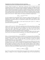
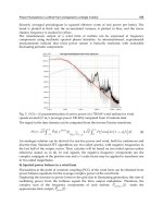
Fig. 3 (left) shows a dead-reckoning path and how it would be used to define the associated
paths of two hypothetical particles. The associated paths Fig. 3 (right) are just versions of the
original path adequately translated and rotated to match the particles’ positions and
headings.

-40 -20 0 20 40 60 80 100
-20
0
20
40
60
80
100
120
140
X
Y
60 80 100 120 140 160 180 200
50
100
150

200
X
Y

Fig. 3. The left picture shows a dead-reckoning path, expressed in a coordinate frame
defined by the position and heading of the last point (red square). The right picture shows
the same path associated to two arbitrary particles, expressed in a common coordinate frame

The new likelihood of a particle is now evaluated through the likelihood of its associated
path with respect to the road map:




 


*
| | ' ',
k
i i
k k k
k
p z X p z t dt







(13)

where


|
k
p z

is the base likelihood of the point

, i.e. likelihood of point

being on the
RNDF map (as defined in (11)).
In order to avoid the effect of time scale (i.e. speed) on the path likelihood, we focus the
evaluation of the likelihood on the intrinsic parameter of the path, integrating over the path
in space and not in time:




 


*
0
| | ,
s
l

i i
k k k
p
z X p z s ds




(14)

where


i
s

is the path expressed in function of its intrinsic parameter
s
and
s
l is the length
of integration over the path. The integration of the hypothetical path can be well
approximated by a discrete summation


 
 
*
1
| |

J
N
i i
k k k j
j
p z X p z s








(15)

where the samples of the intrinsic parameter
j
s
are homogeneously spaced (although that is
not strictly relevant).
Some additional refinements can be considered for the definition of (13), for instance by
considering the direction of the road. This means that the base likelihood would not be just a
function of the position, it would depend on the heading at the points of the path . A path’s
segment that crosses a road would add to the likelihood if where it invades the road it has a
consistent direction (e.g. not a perpendicular one).
Fig. 4 shows an example of a base likelihood (shown as a grayscale image) and particles that
represent the pose of the vehicle and their associated paths (in cyan). The particles’ positions
and headings are represented blue arrows. The red arrow and the red path correspond to
one of most likely hypotheses.

By applying observations that consider the hypothetical past path of the particle, the out-of-
map problem is mitigated (although not solved completely) for transition situations. The
transition between being on the known map and going completely out of it (i.e. current pose
and recent path are out of the map) can be performed safely by considering an approach
based on hysteresis.
The approach is summarized as follows: If the maximum individual path likelihood (the
likelihood of the particle with maximum likelihood) is higher than
H
K
then the process
keeps all particles with likelihood
L
K
 . These thresholds are defined
by
100% 0%
H L
K K   . If the maximum likelihood is
H
K

then the process keeps all the
particles and continues the processing in pure prediction mode. Usual values for these
thresholds are
70%, 60%
H L
K K 
.
RobustGlobalUrbanLocalizationBasedonRoadMaps 275

trajectory




' , ' ,
i
t t k k
 
 
, where the value

defines some horizon of time. This
trajectory ends exactly at the particle instance, i.e.


i i
k
k X

 .
The estimated dead-reckoning trajectory is usually defined in a different coordinate system
as it is the result of an independent process. The important aspect of the dead-reckoning
estimate is that its path has good quality in relative terms, i.e. locally. Its shape is, after
proper rotation and translation, similar to the real path of the vehicle expressed in a
different coordinate frame.
If the dead-reckoning estimate is expressed as the path











' ' , ' , '
i
t x t y t t
  
 
 then the
process to associate it to an individual particle and to express it in the global coordinate
frame is performed according to:


   




 
 
   


     
' , ' , ' , '
' '

i i
k k x y
k
i
k
x
t y t x y R t t
t t k

 
  
   

    
  
(12)

where:



















' , ' ' , ' ,
x y
t t x t y t x k y k
   
    ,




i
k
k k
 
 
   and
R

is a
rotation matrix for a yaw angle

.The angle
i
k


is the heading of the particle
i
k
X
and


k



is the heading of the dead-reckoning path at time k.
Clearly, at time
't k

the difference






' , '
x y
t t  must be


0,0 , and

  

'
' 0
t k
t k
 
 

  ,
consequently
 
'
'
i i
k
t k
t X


 .
Fig. 3 (left) shows a dead-reckoning path and how it would be used to define the associated
paths of two hypothetical particles. The associated paths Fig. 3 (right) are just versions of the
original path adequately translated and rotated to match the particles’ positions and
headings.

-40 -20 0 20 40 60 80 100
-20
0
20
40
60

80
100
120
140
X
Y
60 80 100 120 140 160 180 200
50
100
150
200
X
Y

Fig. 3. The left picture shows a dead-reckoning path, expressed in a coordinate frame
defined by the position and heading of the last point (red square). The right picture shows
the same path associated to two arbitrary particles, expressed in a common coordinate frame

The new likelihood of a particle is now evaluated through the likelihood of its associated
path with respect to the road map:


 
 
 
*
| | ' ',
k
i i
k k k

k
p z X p z t dt



 

(13)

where


|
k
p z

is the base likelihood of the point

, i.e. likelihood of point

being on the
RNDF map (as defined in (11)).
In order to avoid the effect of time scale (i.e. speed) on the path likelihood, we focus the
evaluation of the likelihood on the intrinsic parameter of the path, integrating over the path
in space and not in time:




 



*
0
| | ,
s
l
i i
k k k
p
z X p z s ds




(14)

where


i
s

is the path expressed in function of its intrinsic parameter
s
and
s
l is the length
of integration over the path. The integration of the hypothetical path can be well
approximated by a discrete summation

 
 
*
1
| |
J
N
i i
k k k j
j
p z X p z s


 

 

(15)

where the samples of the intrinsic parameter
j
s
are homogeneously spaced (although that is
not strictly relevant).
Some additional refinements can be considered for the definition of (13), for instance by
considering the direction of the road. This means that the base likelihood would not be just a
function of the position, it would depend on the heading at the points of the path . A path’s
segment that crosses a road would add to the likelihood if where it invades the road it has a

consistent direction (e.g. not a perpendicular one).
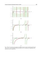
Fig. 4 shows an example of a base likelihood (shown as a grayscale image) and particles that
represent the pose of the vehicle and their associated paths (in cyan). The particles’ positions
and headings are represented blue arrows. The red arrow and the red path correspond to
one of most likely hypotheses.
By applying observations that consider the hypothetical past path of the particle, the out-of-
map problem is mitigated (although not solved completely) for transition situations. The
transition between being on the known map and going completely out of it (i.e. current pose
and recent path are out of the map) can be performed safely by considering an approach
based on hysteresis.
The approach is summarized as follows: If the maximum individual path likelihood (the
likelihood of the particle with maximum likelihood) is higher than
H
K
then the process
keeps all particles with likelihood
L
K
 . These thresholds are defined
by
100% 0%
H L
K K   . If the maximum likelihood is
H
K
 then the process keeps all the
particles and continues the processing in pure prediction mode. Usual values for these
thresholds are
70%, 60%
H L

K K 
.
RobotLocalizationandMapBuilding276

60 80 100 120 140 160 180
40
60
80
100
120
140
160
180
x (meters)
y (meters)

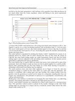
Fig. 4. A synthetic example. This region of interest (ROI) is a rectangle of 200 meters by 200
meters. A set of particles and their associated paths are superimposed to an image of base
likelihood.

In the synthetic example shown in Fig. 4 the region of interest (ROI) is a rectangle of 200
meters by 200 meters. This ROI is big enough to contain the current population of particles
and their associated paths.
Although all the particles are located on the road (high base likelihood); many of their
associated paths abandon the zones of high base likelihood. The most likely particles are
those that have a path mostly contained in the nominal zones. It can be seen the remarkable
effect of a wrong heading that can rotate the associated path and make it to abandon the
zones of high base likelihood (i.e. the road sections in gray).
Some particles have current values that escape the dark gray region (high base likelihood
zones) however their associated paths are mostly contained in the roads. That means the

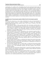
real vehicle could be actually abandoning the road. This situation is repeated in Fig. 5 as
well, where all the particles are located outside of the nominal road although many of them
have paths that match the map constraints.
When the filter infers that the vehicle has been outside the map for sufficient time (i.e. no
particles show relevant part of their paths consistent with the map), no updates are
performed on the particles, i.e. the filter works in pure prediction mode.
When the vehicle enters the known map and eventually there are some particles that
achieve the required path likelihood, i.e. higher than
H
K
, then the filter will start to apply
the updates on the particles.
However this synchronization is not immediate. There could be some delay until some
associated paths are consistent with the map the fact that a particle is well inside the road
does not mean that its likelihood is high. It needs a relevant fraction of its associated path
history to match the road map in order to be considered “inside the map”.

This policy clearly immunizes the filter from bias when incorrect particles are temporarily
on valid roads.
40 60 80 100 120 140 160 180
40
60
80
100
120
140
160
180
x (meters)
y (meters)

Fig. 5. This can be the situation where a vehicle temporarily abandons the road. It can be
seen that although all the particles would have low base likelihood many of them have high
likelihood when their associated paths are considered. Particles outside the road (low Base
Likelihood) but having a correct heading would have high Path Likelihood.

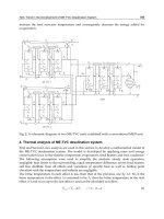
4. Experimental Results
Long term experiments have been performed in urban areas of Sydney. The road maps were
created by an ad-hoc Matlab tool that allowed users to define segments on top of a satellite
image obtained from Google Earth. These road maps were low quality representations of
the roads. This disregard for the quality of the definition of the road maps was done on
purpose with the goal of exposing the approach to realistic and difficult conditions. Fig. 7
and Fig. 8 show the road map used in the estimation process. Fig. 2 shows part of the used
road map as well.
The dead-reckoning process was based on the fusion of speed and heading rate
measurements. The heading rate was provided by low cost three dimensional gyroscopes. A
diversity of additional sensors were available in the platform (PAATV/UTE project)
although those were not used in the estimation process and results presented in this paper.
All the experiments and realistic simulations have validated the satisfactory performance of
the approach.
Figures 7, 8 and 9 present the position estimates as result of the estimation process. Those
are shown in red (Figure 7) or in yellow (Figures 8 and 9) and are superimposed on the road
map. In some parts of the test the vehicle went temporarily outside the known map.
Although there was not a predefined map on those sections it was possible to infer that the
estimator performed adequately. From the satellite image and the over-imposed estimated
path, a human can realize that the estimated path is actually on a road not defined in the a
priori map (Fig. 9).
RobustGlobalUrbanLocalizationBasedonRoadMaps 277

60 80 100 120 140 160 180

40
60
80
100
120
140
160
180
x (meters)
y (meters)

Fig. 4. A synthetic example. This region of interest (ROI) is a rectangle of 200 meters by 200
meters. A set of particles and their associated paths are superimposed to an image of base
likelihood.

In the synthetic example shown in Fig. 4 the region of interest (ROI) is a rectangle of 200
meters by 200 meters. This ROI is big enough to contain the current population of particles
and their associated paths.
Although all the particles are located on the road (high base likelihood); many of their
associated paths abandon the zones of high base likelihood. The most likely particles are
those that have a path mostly contained in the nominal zones. It can be seen the remarkable
effect of a wrong heading that can rotate the associated path and make it to abandon the
zones of high base likelihood (i.e. the road sections in gray).
Some particles have current values that escape the dark gray region (high base likelihood
zones) however their associated paths are mostly contained in the roads. That means the
real vehicle could be actually abandoning the road. This situation is repeated in Fig. 5 as
well, where all the particles are located outside of the nominal road although many of them
have paths that match the map constraints.
When the filter infers that the vehicle has been outside the map for sufficient time (i.e. no
particles show relevant part of their paths consistent with the map), no updates are

performed on the particles, i.e. the filter works in pure prediction mode.
When the vehicle enters the known map and eventually there are some particles that
achieve the required path likelihood, i.e. higher than
H
K
, then the filter will start to apply
the updates on the particles.
However this synchronization is not immediate. There could be some delay until some
associated paths are consistent with the map the fact that a particle is well inside the road
does not mean that its likelihood is high. It needs a relevant fraction of its associated path
history to match the road map in order to be considered “inside the map”.

This policy clearly immunizes the filter from bias when incorrect particles are temporarily
on valid roads.
40 60 80 100 120 140 160 180
40
60
80
100
120
140
160
180
x (meters)
y (meters)

Fig. 5. This can be the situation where a vehicle temporarily abandons the road. It can be
seen that although all the particles would have low base likelihood many of them have high
likelihood when their associated paths are considered. Particles outside the road (low Base
Likelihood) but having a correct heading would have high Path Likelihood.

4. Experimental Results
Long term experiments have been performed in urban areas of Sydney. The road maps were
created by an ad-hoc Matlab tool that allowed users to define segments on top of a satellite
image obtained from Google Earth. These road maps were low quality representations of
the roads. This disregard for the quality of the definition of the road maps was done on
purpose with the goal of exposing the approach to realistic and difficult conditions. Fig. 7
and Fig. 8 show the road map used in the estimation process. Fig. 2 shows part of the used
road map as well.
The dead-reckoning process was based on the fusion of speed and heading rate
measurements. The heading rate was provided by low cost three dimensional gyroscopes. A
diversity of additional sensors were available in the platform (PAATV/UTE project)
although those were not used in the estimation process and results presented in this paper.
All the experiments and realistic simulations have validated the satisfactory performance of
the approach.
Figures 7, 8 and 9 present the position estimates as result of the estimation process. Those
are shown in red (Figure 7) or in yellow (Figures 8 and 9) and are superimposed on the road
map. In some parts of the test the vehicle went temporarily outside the known map.
Although there was not a predefined map on those sections it was possible to infer that the
estimator performed adequately. From the satellite image and the over-imposed estimated
path, a human can realize that the estimated path is actually on a road not defined in the a
priori map (Fig. 9).
RobotLocalizationandMapBuilding278

It is difficult to define a true path in order to compare it with the estimated solution. This is
because the estimator is intended to provide permanent global localization with a quality
usually similar to a GPS. Figures 10, 11 and 12 present the estimated positions and
corresponding GPS estimates although those were frequently affected by multipath and
other problems.

5. Conclusions and Future Work
This paper presented a method to perform global localization in urban environments using
segment-based maps together with particle filters. In the proposed approach the likelihood
function is locally generated as a grid derived from segment-based maps. The scheme can
efficiently assign weights to the particles in real time, with minimum memory requirements
and without any additional pre-filtering procedures. Multi-hypothesis cases are handled
transparently by the filter. A path-based observation model is developed as an extension to
consistently deal with out-of-map navigation cases. This feature is highly desirable since the
map can be incomplete, or the vehicle can be actually located outside the boundaries of the
provided map.
The system behaves like a virtual GPS, providing accurate global localization without using
an actual GPS.
Experimental results have shown that the proposed architecture works robustly in urban
environments using segment-based road maps. These particular maps provide road
network connectivity in the context of the Darpa Urban Challenge. However, the proposed
architecture is general and can be used with any kind of segment-based or topological a
priori map.
The filter is able to provide consistent localization, for extended periods of time and long
traversed courses, using only rough dead-reckoning input (affected by considerably drift),
and the RNDF map.
The system performs robustly in a variety of circumstances, including extreme situations
such as tunnels, where a GPS-based positioning would not render any solution at all.
The continuation of this work involves different lines of research and development. One of
them is the implementation of this approach as a robust and reliable module ready to be
used as a localization resource by other systems. However this process should be flexible
enough to allow the integration with other sources of observations such as biased compass
measurements and even sporadic GPS measurements.
Other necessary and interesting lines are related to the initialization of the estimation
process, particularly for cases where the robot starts at a completely unknown position.
Defining a huge local area for the definition of the likelihood (and spreading a population of

particles in it) is not feasible in real-time. We are investigating efficient and practical
solutions for that issue.
Another area of relevance is the application of larger paths in the evaluation of the Path
Likelihood. In the current implementation we consider a deterministic path, i.e. we exploit
the fact that for short paths the dead-reckoning presents low uncertainty to the degree of
allowing us to consider the recent path as a deterministic entity. In order to extend the path
validity we need to model the path in a stochastic way, i.e. by a PDF. Although this concept
is mathematically easy to define and understand it implies considerable additional
computational cost.

Finally, the observability of the estimation process can be increased by considering
additional sources of observation such the detection of road intersections. These additional
observations would improve the observability of the process particularly when the vehicle
does not perform turning maneuvers for long periods.

Likelihood in selected region
longitude, Km
latitude, Km
1.15 1.2 1.25 1.3 1.35 1.4 1.45 1.5 1.55
2
2.05
2.1
2.15
2.2
2.25
2.3

Fig. 6. A local base likelihood automatically created. This ROI is defined to be the smallest
rectangle that contains the hypothetical histories of all the current particles. The different
colors mean different lanes although that property was not used in the definition of the base

likelihood for the experiment presented in this paper.

-1500 -1000 -500 0 500 1000 1500 2000
-1500
-1000
-500
0
500
1000
1500
2000
2500
Estimated Path and Known Map
longitude (m)
latitude (m)

Fig. 7. Field test through Sydney. The system never gets lost. Even feeding the real-time
system lower quality measurements (by playing back data corrupted with additional noise)
and removing sections of roads from the a-priori map) the results are satisfactory. The red
lines are the obtained solution for a long trip.
RobustGlobalUrbanLocalizationBasedonRoadMaps 279

It is difficult to define a true path in order to compare it with the estimated solution. This is
because the estimator is intended to provide permanent global localization with a quality
usually similar to a GPS. Figures 10, 11 and 12 present the estimated positions and
corresponding GPS estimates although those were frequently affected by multipath and
other problems.

5. Conclusions and Future Work
This paper presented a method to perform global localization in urban environments using

segment-based maps together with particle filters. In the proposed approach the likelihood
function is locally generated as a grid derived from segment-based maps. The scheme can
efficiently assign weights to the particles in real time, with minimum memory requirements
and without any additional pre-filtering procedures. Multi-hypothesis cases are handled
transparently by the filter. A path-based observation model is developed as an extension to
consistently deal with out-of-map navigation cases. This feature is highly desirable since the
map can be incomplete, or the vehicle can be actually located outside the boundaries of the
provided map.
The system behaves like a virtual GPS, providing accurate global localization without using
an actual GPS.
Experimental results have shown that the proposed architecture works robustly in urban
environments using segment-based road maps. These particular maps provide road
network connectivity in the context of the Darpa Urban Challenge. However, the proposed
architecture is general and can be used with any kind of segment-based or topological a
priori map.
The filter is able to provide consistent localization, for extended periods of time and long
traversed courses, using only rough dead-reckoning input (affected by considerably drift),
and the RNDF map.
The system performs robustly in a variety of circumstances, including extreme situations
such as tunnels, where a GPS-based positioning would not render any solution at all.
The continuation of this work involves different lines of research and development. One of
them is the implementation of this approach as a robust and reliable module ready to be
used as a localization resource by other systems. However this process should be flexible
enough to allow the integration with other sources of observations such as biased compass
measurements and even sporadic GPS measurements.
Other necessary and interesting lines are related to the initialization of the estimation
process, particularly for cases where the robot starts at a completely unknown position.
Defining a huge local area for the definition of the likelihood (and spreading a population of
particles in it) is not feasible in real-time. We are investigating efficient and practical
solutions for that issue.

Another area of relevance is the application of larger paths in the evaluation of the Path
Likelihood. In the current implementation we consider a deterministic path, i.e. we exploit
the fact that for short paths the dead-reckoning presents low uncertainty to the degree of
allowing us to consider the recent path as a deterministic entity. In order to extend the path
validity we need to model the path in a stochastic way, i.e. by a PDF. Although this concept
is mathematically easy to define and understand it implies considerable additional
computational cost.

Finally, the observability of the estimation process can be increased by considering
additional sources of observation such the detection of road intersections. These additional
observations would improve the observability of the process particularly when the vehicle
does not perform turning maneuvers for long periods.

Likelihood in selected region
longitude, Km
latitude, Km
1.15 1.2 1.25 1.3 1.35 1.4 1.45 1.5 1.55
2
2.05
2.1
2.15
2.2
2.25
2.3

Fig. 6. A local base likelihood automatically created. This ROI is defined to be the smallest
rectangle that contains the hypothetical histories of all the current particles. The different
colors mean different lanes although that property was not used in the definition of the base
likelihood for the experiment presented in this paper.

-1500 -1000 -500 0 500 1000 1500 2000
-1500
-1000
-500
0
500
1000
1500
2000
2500
Estimated Path and Known Map
longitude (m)
latitude (m)

Fig. 7. Field test through Sydney. The system never gets lost. Even feeding the real-time
system lower quality measurements (by playing back data corrupted with additional noise)
and removing sections of roads from the a-priori map) the results are satisfactory. The red
lines are the obtained solution for a long trip.
RobotLocalizationandMapBuilding280

-1500 -1000 -500 0 500 1000 1500 2000
-1000
-500
0
500
1000
1500
2000
2500
Longitude (m)

Latitude (m)

Fig. 8. Estimated path (in yellow) for one of the experiments. The known map (cyan) and a
satellite image of the region are included in the picture.
1000 1100 1200 1300 1400 1500 1600 1700 1800 1900 2000
500
600
700
800
900
1000
1100
1200
1300
Longitude (m)
Latitude (m)

Fig. 9. A section of Fig. 8 where the solution is consistent even where the map is incomplete
(approximately x=1850m, y=1100m).

1000 1100 1200 1300 1400 1500 1600 1700 1800 1900 2000
-800
-750
-700
-650
-600
-550
Longitude (m)
Latitude (m)

Fig. 10. A comparison between the estimated solution and the available GPS measurements.
The green dots are the estimated solution and the blue ones correspond to GPS
measurements. The segments in cyan connect samples of GPS and their corresponding
estimated positions (i.e. exactly for the same sample time). The blue lines are the map’s
segments.
1550 1600 1650 1700 1750
-800
-790
-780
-770
-760
-750
-740
Longitude (m)
Latitude (m)

Fig. 11. A detailed view of Figure 10. It is clear that the GPS’ measurements present jumps
and other inconsistencies.
RobustGlobalUrbanLocalizationBasedonRoadMaps 281

-1500 -1000 -500 0 500 1000 1500 2000
-1000
-500
0
500
1000
1500
2000
2500
Longitude (m)

Latitude (m)

Fig. 8. Estimated path (in yellow) for one of the experiments. The known map (cyan) and a
satellite image of the region are included in the picture.
1000 1100 1200 1300 1400 1500 1600 1700 1800 1900 2000
500
600
700
800
900
1000
1100
1200
1300
Longitude (m)
Latitude (m)

Fig. 9. A section of Fig. 8 where the solution is consistent even where the map is incomplete
(approximately x=1850m, y=1100m).

1000 1100 1200 1300 1400 1500 1600 1700 1800 1900 2000
-800
-750
-700
-650
-600
-550
Longitude (m)
Latitude (m)

Fig. 10. A comparison between the estimated solution and the available GPS measurements.
The green dots are the estimated solution and the blue ones correspond to GPS
measurements. The segments in cyan connect samples of GPS and their corresponding
estimated positions (i.e. exactly for the same sample time). The blue lines are the map’s
segments.
1550 1600 1650 1700 1750
-800
-790
-780
-770
-760
-750
-740
Longitude (m)
Latitude (m)

Fig. 11. A detailed view of Figure 10. It is clear that the GPS’ measurements present jumps
and other inconsistencies.
RobotLocalizationandMapBuilding282

1680 1690 1700 1710 1720 1730
-788
-786
-784
-782
-780
-778
-776
-774
-772

-770
Longitude (m)
Latitude (m)

Fig. 12. A close inspection shows interesting details. The estimates are provided at
frequencies higher than the GPS (5Hz). The GPS presents jumps and the road segment
appears as a continuous piece-wise line (in blue), both sources of information are unreliable
if used individually.

6. References
S. Arulampalam, S. Maskell, N. Gordon, and T. Clapp, “A Tutorial on Particle Filters for On-
line Non-linear/Non-Gaussian Bayesian Tracking,” IEEE Transactions on Signal
Processing, vol. 50, no. 2, pp. 174–188, 2002.
F. Dellaert, D. Fox, W. Burgard, and S. Thrun, “Monte Carlo Localization for Mobile
Robots,” in International Conference on Robotics and Automation. Detroit: IEEE, 1999.
D. Fox, S. Thrun, W. Burgard, and F. Dellaert, “Particle Filters for Mobile Robot
Localization,” in Sequential Monte Carlo Methods in Practice, A. Doucet, N. de Freitas,
and Gordon, Eds. New York: Springer, 2001.
J. E. Guivant and E. M. Nebot, “Optimization of the Simultaneous Localization and Map-
building Algorithm for Real time Implementation,” IEEE Transactions on Robotics
and Automation, vol. 17, no. 3, 2001, pp. 242–257.
J. Guivant, and R. Katz, “Global urban localization based on road maps,” in RSJ
International Conference on Intelligent Robots and Systems, IROS. San Diego, CA :
IEEE, Oct. 2007, pp 1079-1084. ISBN: 978-1-4244-0912-9.
J. J. Leonard and H. F. Durrant-Whyte, “Simultaneous Map Building and Localization for an
Autonomous Mobile Robot,” IEEE/RSJ International Workshop on Intelligent Robots
and Systems. IEEE, 1991.

L. Liao, D. Fox, J. Hightower, H. Kautz, and D. Schultz, “Voronoi Tracking: Location
Estimation Using Sparse and Noisy Sensor Data,” in IEEE/RSJ International

Workshop on Intelligent Robots and Systems. Las Vegas, USA: IEEE, 2003.
M. E. E. Najjar and P. Bonnifait, “A Road-Matching Method for Precise Vehicle Localization
Using Belief Theory and Kalman Filtering,” Autonomous Robots, vol. 19, no. 2, 2005,
pp. 173–191.
S. M. Oh, S. Tariq, B. N. Walker, and F. Dellaert, “Map based Priors for Localization,” in
IEEE/RSJ International Workshop on Intelligent Robots and Systems. Sendai, Japan:
IEEE, 2004.
G. Taylor and G. Blewitt, “Road Reduction Filtering using GPS,” in 3rd AGILE Conference on
Geographic Information Science, Helsinki, Finland, 2000.
ACFR, The University of Sydney and LCR, Universidad Nacional del Sur, “PAATV/UTE
Projects,” Sydney, Australia, 2006.
Defence Advanced Research Projects Agency (DARPA), “DARPA Urban Challenge,”
2006.
Google, “Google Earth,” 2007.
RobustGlobalUrbanLocalizationBasedonRoadMaps 283

1680 1690 1700 1710 1720 1730
-788
-786
-784
-782
-780
-778
-776
-774
-772
-770
Longitude (m)
Latitude (m)

Fig. 12. A close inspection shows interesting details. The estimates are provided at
frequencies higher than the GPS (5Hz). The GPS presents jumps and the road segment
appears as a continuous piece-wise line (in blue), both sources of information are unreliable
if used individually.

6. References
S. Arulampalam, S. Maskell, N. Gordon, and T. Clapp, “A Tutorial on Particle Filters for On-
line Non-linear/Non-Gaussian Bayesian Tracking,” IEEE Transactions on Signal
Processing, vol. 50, no. 2, pp. 174–188, 2002.
F. Dellaert, D. Fox, W. Burgard, and S. Thrun, “Monte Carlo Localization for Mobile
Robots,” in International Conference on Robotics and Automation. Detroit: IEEE, 1999.
D. Fox, S. Thrun, W. Burgard, and F. Dellaert, “Particle Filters for Mobile Robot
Localization,” in Sequential Monte Carlo Methods in Practice, A. Doucet, N. de Freitas,
and Gordon, Eds. New York: Springer, 2001.
J. E. Guivant and E. M. Nebot, “Optimization of the Simultaneous Localization and Map-
building Algorithm for Real time Implementation,” IEEE Transactions on Robotics
and Automation, vol. 17, no. 3, 2001, pp. 242–257.
J. Guivant, and R. Katz, “Global urban localization based on road maps,” in RSJ
International Conference on Intelligent Robots and Systems, IROS. San Diego, CA :
IEEE, Oct. 2007, pp 1079-1084. ISBN: 978-1-4244-0912-9.
J. J. Leonard and H. F. Durrant-Whyte, “Simultaneous Map Building and Localization for an
Autonomous Mobile Robot,” IEEE/RSJ International Workshop on Intelligent Robots
and Systems. IEEE, 1991.

L. Liao, D. Fox, J. Hightower, H. Kautz, and D. Schultz, “Voronoi Tracking: Location
Estimation Using Sparse and Noisy Sensor Data,” in IEEE/RSJ International
Workshop on Intelligent Robots and Systems. Las Vegas, USA: IEEE, 2003.
M. E. E. Najjar and P. Bonnifait, “A Road-Matching Method for Precise Vehicle Localization
Using Belief Theory and Kalman Filtering,” Autonomous Robots, vol. 19, no. 2, 2005,
pp. 173–191.

S. M. Oh, S. Tariq, B. N. Walker, and F. Dellaert, “Map based Priors for Localization,” in
IEEE/RSJ International Workshop on Intelligent Robots and Systems. Sendai, Japan:
IEEE, 2004.
G. Taylor and G. Blewitt, “Road Reduction Filtering using GPS,” in 3rd AGILE Conference on
Geographic Information Science, Helsinki, Finland, 2000.
ACFR, The University of Sydney and LCR, Universidad Nacional del Sur, “PAATV/UTE
Projects,” Sydney, Australia, 2006.
Defence Advanced Research Projects Agency (DARPA), “DARPA Urban Challenge,”
2006.
Google, “Google Earth,” 2007.
RobotLocalizationandMapBuilding284
ObjectLocalizationusingStereoVision 285
ObjectLocalizationusingStereoVision
SaiKrishnaVuppala
x

Object Localization using Stereo Vision

Sai Krishna Vuppala
Institute of Automation, University of Bremen
Germany

1. Introduction

Computer vision is the science and technology of machines that see. The theoretical
explanation about the optics of the eye and the information about the existence of images
formed at the rear of the eye ball are provided by Kepler and Scheiner respectively in the
16th century (Lin, 2002). The field of computer vision is started emerging in the second half
of 19th century, since then researchers have been trying to develop the methods and systems
aiming at imitating the biological vision process and therefore increasing the machine

intelligence for many possible applications in the real world. The theoretical knowledge
behind the perception of 3D real world using multiple vision systems has been published in
various literature, and (
Hartley & Zisserman 2000) (Klette at al., 1998) (Sterger , 2007) are few
well known from them. As there are numerous applications of computer vision in service,
industrial, surveillance, and surgical etc automation sectors, researchers have been
publishing numerous methods and systems that address their specific goals. It is intended
with most of these researchers that their developed methods and systems are enough
general with respect to the aspects such as functional, robust, time effective and safety
issues. Though practical limitations hinder the researchers and developers in achieving
these goals, many are getting ahead providing the solutions to the known and predicted
problems.
The field of computer vision is supporting the field of robotics with many vision based
applications. In service robotics action interpretation and object manipulation are few
examples with which the computer vision supports the humans. According to (Taylor &
Kleeman, 2006), three things are almost certain about universal service robots of the future:
many will have manipulators (and probably legs!), most will have cameras, and almost all
will be called upon to grasp, lift, carry, stack or otherwise manipulate objects in our
environment. Visual perception and coordination in support of robotic grasping is thus a
vital area of research for the progress of universal service robots. Service robotic tasks are
usually specified at a supervisory level with reference to general actions and classes of
objects. An example of such a task would be: Please get ‘the bottle’ from ‘the fridge’. Here,
getting the bottle is the intended action, ‘bottle’ belongs to the class of objects that are
manipulated, and ‘fridge’ belongs to the class of objects in/on which the objects to be
manipulated lie. The content of the manuscript addresses the object manipulation tasks
using stereo vision for applications of service robotics. Motivation of the content of the
manuscript stems from the needs of service robotic systems FRIEND II and FRIEND III
15
RobotLocalizationandMapBuilding286

(Functional Robot with dexterous arm and user-frIENdly interface for Disabled people) that
are being developed at IAT (Institute of Automation, University of Bremen, Germany). The
systems FRIEND II and FRIEND III are shown in figure 1 a) and b). The objects of interest to
be manipulated are shown in figure 2.


Fig. 1. Rehabilitation robotic systems a) FRIEND II b) FRIEND III


Fig. 2. The objects of interest for the manipulation purpose

In order robot manipulators to perform their actions autonomously, 3D environment
information is necessary. In order to reconstruct 3D object information using cameras
various approaches have been investigated since few decades. According to (Lange at al.,
2006), the 3D object information recovery techniques are broadly classified into passive and
active sensing methods. Passive sensing methods require relatively low power compared to
the active methods. Passive sensing methods are similar to the biological vision process. The
characteristic contrast-related features in images (i.e. cues such as shading, texture) of the

observed scene are used in extracting the 3D information. In active sensing methods
compared with passive methods high accuracy measurements can be obtained. Active
sensing relies on projecting energy into the environment and interpreting the modified
sensory view. CMOS time-of-flight cameras can capture complete 3D image in a single
measurement cycle (Lange, 2000), however such a technology is limited with timing
resolutions and, the possibility of the 3D information perception depends on the object
surface properties.
Considering passive sensing methods, though any number of cameras can be used in 3D
vision process, the methods based on stereo vision plays optimal role considering the
functional, hardware, and computational issues. Visual servoing system (Corke, 1996)
(

Hutchinson, 1996) come into this this category. The two major classes of such systems are
position- and image based visual servoing systems. In position based visual servoing
systems, they are further classified into closed- and open loop systems. Depending on the
requirements of the strategy, they can be realized using single, or two cameras. Closed loop
systems have high accuracy since the overall system error is minimized using the feedback
information, where as in an open-loop system the error depends on the performance of the
system in a single step. In contrast to the closed approaches look-then-move is an open loop
approach for the autonomous task executions; the vision system identifies the target location
in 3D and the robot is driven to the location of interest. In look-then-move approach, the
accuracy of the overall robotic system depends on the camera calibration accuracy and the
manipulator accuracy in reaching the specified locations in the real world (
Garric & Devy
1995
). In a system like FRIEND II look-then-move approach is prefered since object
manipulation, collision avoidance, and path planning are planned using a standlone stereo
camera unit.
Stereo triangulation is the core process in stereo based 3D vision applications, in order to
calculate 3D point stereo correspondences information is used. Precisely identified stereo
correspondences give precise 3D reconstruction results. Any uncertainty in the result of
stereo correspondences can potentially yield a virtually unbounded uncertainty in the result
of 3D reconstruction (Lin, 2002). Precise 3D reconstruction additionally requires well
calibrated stereo cameras as the calibrated parameters of the stereo view geometry are used
in the stereo triangulation process (
Hartley & Zissermann 2000). In addition to that 3D
reconstruction accuracy further depends on the length of base line (Gilbert at al., 2006), if the
base line is shorter the matching process is facilitated, and if the base line is larger the 3D
reconstruction accuracy is higher. Approaches for finding the stereo correspondences are
broadly classified into two types (
Klette at al., 1998); they are intensity and feature-based
matching techniques. The state of the art stereo correspondence search algorithms mostly

based on various scene and geometry based constraints. These algorithms can not be used
for the texture less objects as the reconstructed obejct information is error prone.
The pose (position and orientation) of an object can be estimated using the information from
a single or multiple camera views. Assuming that the internal camera parameters are
known, the problem of finding the object pose is nothing but finding the orientation and
position of object with respect to the camera. The problem of finding the pose of the object
using the image and object point correspondences in the literature is described as a
perspective n-point problem. The standard perspective n-point problem can be solved using
systems of linear equations if correspondences between at least six image and scene points
are known. Several researchers provided solutions for this problem considering at least 3
ObjectLocalizationusingStereoVision 287

(Functional Robot with dexterous arm and user-frIENdly interface for Disabled people) that
are being developed at IAT (Institute of Automation, University of Bremen, Germany). The
systems FRIEND II and FRIEND III are shown in figure 1 a) and b). The objects of interest to
be manipulated are shown in figure 2.


Fig. 1. Rehabilitation robotic systems a) FRIEND II b) FRIEND III


Fig. 2. The objects of interest for the manipulation purpose

In order robot manipulators to perform their actions autonomously, 3D environment
information is necessary. In order to reconstruct 3D object information using cameras
various approaches have been investigated since few decades. According to (Lange at al.,
2006), the 3D object information recovery techniques are broadly classified into passive and
active sensing methods. Passive sensing methods require relatively low power compared to
the active methods. Passive sensing methods are similar to the biological vision process. The
characteristic contrast-related features in images (i.e. cues such as shading, texture) of the

observed scene are used in extracting the 3D information. In active sensing methods
compared with passive methods high accuracy measurements can be obtained. Active
sensing relies on projecting energy into the environment and interpreting the modified
sensory view. CMOS time-of-flight cameras can capture complete 3D image in a single
measurement cycle (Lange, 2000), however such a technology is limited with timing
resolutions and, the possibility of the 3D information perception depends on the object
surface properties.
Considering passive sensing methods, though any number of cameras can be used in 3D
vision process, the methods based on stereo vision plays optimal role considering the
functional, hardware, and computational issues. Visual servoing system (Corke, 1996)
(
Hutchinson, 1996) come into this this category. The two major classes of such systems are
position- and image based visual servoing systems. In position based visual servoing
systems, they are further classified into closed- and open loop systems. Depending on the
requirements of the strategy, they can be realized using single, or two cameras. Closed loop
systems have high accuracy since the overall system error is minimized using the feedback
information, where as in an open-loop system the error depends on the performance of the
system in a single step. In contrast to the closed approaches look-then-move is an open loop
approach for the autonomous task executions; the vision system identifies the target location
in 3D and the robot is driven to the location of interest. In look-then-move approach, the
accuracy of the overall robotic system depends on the camera calibration accuracy and the
manipulator accuracy in reaching the specified locations in the real world (
Garric & Devy
1995
). In a system like FRIEND II look-then-move approach is prefered since object
manipulation, collision avoidance, and path planning are planned using a standlone stereo
camera unit.
Stereo triangulation is the core process in stereo based 3D vision applications, in order to
calculate 3D point stereo correspondences information is used. Precisely identified stereo

correspondences give precise 3D reconstruction results. Any uncertainty in the result of
stereo correspondences can potentially yield a virtually unbounded uncertainty in the result
of 3D reconstruction (Lin, 2002). Precise 3D reconstruction additionally requires well
calibrated stereo cameras as the calibrated parameters of the stereo view geometry are used
in the stereo triangulation process (
Hartley & Zissermann 2000). In addition to that 3D
reconstruction accuracy further depends on the length of base line (Gilbert at al., 2006), if the
base line is shorter the matching process is facilitated, and if the base line is larger the 3D
reconstruction accuracy is higher. Approaches for finding the stereo correspondences are
broadly classified into two types (
Klette at al., 1998); they are intensity and feature-based
matching techniques. The state of the art stereo correspondence search algorithms mostly
based on various scene and geometry based constraints. These algorithms can not be used
for the texture less objects as the reconstructed obejct information is error prone.
The pose (position and orientation) of an object can be estimated using the information from
a single or multiple camera views. Assuming that the internal camera parameters are
known, the problem of finding the object pose is nothing but finding the orientation and
position of object with respect to the camera. The problem of finding the pose of the object
using the image and object point correspondences in the literature is described as a
perspective n-point problem. The standard perspective n-point problem can be solved using
systems of linear equations if correspondences between at least six image and scene points
are known. Several researchers provided solutions for this problem considering at least 3
RobotLocalizationandMapBuilding288

object points. According to Shakunaga in his publication on pose estimation using single
camera (
Shakunaga, 1991) described that an n-vector body with n >=3 gives at most 8 rotation
candidates from object image correspondences. In case if n < 3, the recovery of the rotation
of n-vector body is not possible.
The content of the manuscript discusses selection of stereo feature correspondences and

determining the stereo correspondences for opted features on texture less objects in sections
2 and 3 respectively; section 4 presents tracking object pose using 2 object points. ; section 5
presents 3D object reconstruction results; Conclusion and References are followed in
sections 6 and 7 respectively.

2. Selection of Stereo Feature Correspondences

Scene independent 3D object reconstruction requires information from at least two camera
views. Considering stereo vision rather than multiple vision systems for this purpose eases
the computational complexity of the system. Stereo vision based 3D reconstruction methods
require stereo correspondence information. Traditional problems in finding the stereo
correspondence are occlusion, regularity/ repetitiveness. Traditionally these problems are
solved using intensity and feature based stereo matching techniques. However, absolute
homogeneous surfaces without any sharp features (i.e. edges, corners etc) do not provide
proper stereo correspondence information. The domestic objects to be manipulated in the
FRIEND environment are some examples of such kind. As the considered object (either each
part or the whole body) has uniform color information the intensity based correspondence
search methods often provide improper stereo correspondence information. Therefoere,
alternatively the edges of the green bottle are observed for the stereo correspondence
analysis. Out of all possible edges of green bottle that is shown in figure 3, only the
orientation edges of the bottle can be considered for the 3D bottle reconstruction; this is
because the stereo correspondence information between other kinds of edges is typically
lost.

2.1 Resolutions between 3D and 2D
The 3D reconstruction accuracy depends on, the accuracy of calibration parameters, the sub
pixel accuracy of stereo correspondences and the length of the baseline. In addition to these
factors, the 3D reconstruction accuracy further depends on the pixel size, the focal length of
the camera, and the distance between the camera and the object. In the following the feasible
spatial resolution of object surface in the projected scene is analyzed. Figure 4 illustrates the

projection of the object surface on to a single image row. The feasible geometrical resolution
of the object surface projected on to one row of the image plane is calculated using formula
(1). Similarly the feasible resolution of the object projection on to the column of the object
plane can be calculated. The width and the height of the pictured scene are also can be
approximately calculated multiplying the number of pixels along the rows and columns
multiplied with respective feasible resolutions.


Fig. 3. Various possible edges of green bottle from FRIEND Environment

f
pd
resolutionfeasible 

(1)


Fig. 4. Feasible spatial resolution on object surface in the projected scene (Klette at al., 1998)

E.g: The size of the SONY CCD Sensor ICX204AK that is used in the bumblebee stereo
vision system has the pixel size of 4.54

m×4.54

m, the focal length of the camera is 4mm,
and the assumed situation of the object is about 1m far from the camera. The feasible
resolution of the camera along the row is 1.125mm/column and the feasible resolution along
the column is 1.125mm/row. Similarly with a higher focal length camera such as 6mm the
feasible resolution becomes 0.75mm/column. Implicitely, with decrease in feasible
resolution increases the 3D reconstruction accuracy. From equation (1), the feasible

resolution is proportional to the distance between the camera and the object, as the distance
ObjectLocalizationusingStereoVision 289

object points. According to Shakunaga in his publication on pose estimation using single
camera (
Shakunaga, 1991) described that an n-vector body with n >=3 gives at most 8 rotation
candidates from object image correspondences. In case if n < 3, the recovery of the rotation
of n-vector body is not possible.
The content of the manuscript discusses selection of stereo feature correspondences and
determining the stereo correspondences for opted features on texture less objects in sections
2 and 3 respectively; section 4 presents tracking object pose using 2 object points. ; section 5
presents 3D object reconstruction results; Conclusion and References are followed in
sections 6 and 7 respectively.

2. Selection of Stereo Feature Correspondences

Scene independent 3D object reconstruction requires information from at least two camera
views. Considering stereo vision rather than multiple vision systems for this purpose eases
the computational complexity of the system. Stereo vision based 3D reconstruction methods
require stereo correspondence information. Traditional problems in finding the stereo
correspondence are occlusion, regularity/ repetitiveness. Traditionally these problems are
solved using intensity and feature based stereo matching techniques. However, absolute
homogeneous surfaces without any sharp features (i.e. edges, corners etc) do not provide
proper stereo correspondence information. The domestic objects to be manipulated in the
FRIEND environment are some examples of such kind. As the considered object (either each
part or the whole body) has uniform color information the intensity based correspondence
search methods often provide improper stereo correspondence information. Therefoere,
alternatively the edges of the green bottle are observed for the stereo correspondence
analysis. Out of all possible edges of green bottle that is shown in figure 3, only the
orientation edges of the bottle can be considered for the 3D bottle reconstruction; this is

because the stereo correspondence information between other kinds of edges is typically
lost.

2.1 Resolutions between 3D and 2D
The 3D reconstruction accuracy depends on, the accuracy of calibration parameters, the sub
pixel accuracy of stereo correspondences and the length of the baseline. In addition to these
factors, the 3D reconstruction accuracy further depends on the pixel size, the focal length of
the camera, and the distance between the camera and the object. In the following the feasible
spatial resolution of object surface in the projected scene is analyzed. Figure 4 illustrates the
projection of the object surface on to a single image row. The feasible geometrical resolution
of the object surface projected on to one row of the image plane is calculated using formula
(1). Similarly the feasible resolution of the object projection on to the column of the object
plane can be calculated. The width and the height of the pictured scene are also can be
approximately calculated multiplying the number of pixels along the rows and columns
multiplied with respective feasible resolutions.


Fig. 3. Various possible edges of green bottle from FRIEND Environment

f
pd
resolutionfeasible 

(1)


Fig. 4. Feasible spatial resolution on object surface in the projected scene (Klette at al., 1998)

E.g: The size of the SONY CCD Sensor ICX204AK that is used in the bumblebee stereo
vision system has the pixel size of 4.54


m×4.54

m, the focal length of the camera is 4mm,
and the assumed situation of the object is about 1m far from the camera. The feasible
resolution of the camera along the row is 1.125mm/column and the feasible resolution along
the column is 1.125mm/row. Similarly with a higher focal length camera such as 6mm the
feasible resolution becomes 0.75mm/column. Implicitely, with decrease in feasible
resolution increases the 3D reconstruction accuracy. From equation (1), the feasible
resolution is proportional to the distance between the camera and the object, as the distance
RobotLocalizationandMapBuilding290

between the object and the camera decreases the feasible resolution for the object decreases
and therefore increases the accuracy of 3D reconstruction processes.

2.2 Stereo Feature Correspondences for Homogeneous Object Surfaces
For a pair of matching line segments in stereo images, any point on the first line segment can
correspond to every other point on the second line segment, and this ambiguity can only be
resolved if the end-points of the two line segments are known exactly. Consider that the line
segment AB shown in figure 5 lies on a cylindrical object surface is identified in stereo
images. The stereo correspondences for the end points A and B are considered to be
available. As no other external object hides the object line, all the projected object points on
line AB have corresponding stereo image pixels.


Fig. 5. a) Line segment on the object surface which could be identified in stereo images; b)
Significant view of the line segment for the stereo correspondence analysis

It is not always possible to have (or detect) such line segments on the objects whose end
points stereo correspondences could be determined. Therefore as an alternative, the points

on the object contour (the edges of the object boundary that represent object shape in
images) are considered for the stereo correspondence analysis. Surface curvature of an
object is inversely proportional to the square of its radius. If the object surface curvature is
not equal to zero the visible object contours in stereo images though may appear similar but
do not correspond to the same object points. Figures 6a and 6b show the cross sections of
object surfaces with different radius of curvatures observed from two different positions,
object indexed with 1 has low surface curvature and object indexed with 2 has high radius of
curvature. In figures 6a and 6b, the points A and B are any two points obtained from the
contour image of the left camera for object indexed 1, and A’ and B’ are the similar points
obtained for object indexed 1 from the contour image of the right camera; similarly, points P
and Q are any two points obtained from the contour image of the left camera for object

indexed 2, and P’ and Q’ are similar points obtained for object indexed 2 from the contour
image of the right camera. Though (A,A’), (B,B’), (P,P’) and (Q,Q’) do not give real
correspondences, an approximation of the reconstructed information is not far from the real
3D values. Also, intuitively one can say that the selected points from the high surface
curvature give more appropriate stereo correspondences. Therefore if objects do not provide
intensity or feature based stereo correspondence information, geometric specific feature
points on object surfaces with larger radius of curvatures can be considered in order to have
less 3D reconstruction errors. As the considered domestic objects within the FRIEND
environment are texture less, approach discussed as above has been used to reconstruct the
objects. Figure 7 shows the selection of contour regions in order to have less stereo
correspondence errors for the objects that are intended to be manipulated in the FRIEND
environment (bottle and meal tray). The contour area marked in the Fig 7a has the high
radius of curvature on the surface of the green bottle. In case of the meal tray, as we have
considered to reconstruct the meal tray using the red handle (shown in Fig 7b), the marked
contour area of the meal tray has the high radius of curvature. Therefore in order to
reconstruct these objects feature points are extracted from the marked contour object
regions.

Fig. 6. object surfaces with different radius of curvatures from two different views

ObjectLocalizationusingStereoVision 291

between the object and the camera decreases the feasible resolution for the object decreases
and therefore increases the accuracy of 3D reconstruction processes.

2.2 Stereo Feature Correspondences for Homogeneous Object Surfaces
For a pair of matching line segments in stereo images, any point on the first line segment can
correspond to every other point on the second line segment, and this ambiguity can only be
resolved if the end-points of the two line segments are known exactly. Consider that the line
segment AB shown in figure 5 lies on a cylindrical object surface is identified in stereo
images. The stereo correspondences for the end points A and B are considered to be
available. As no other external object hides the object line, all the projected object points on
line AB have corresponding stereo image pixels.


Fig. 5. a) Line segment on the object surface which could be identified in stereo images; b)
Significant view of the line segment for the stereo correspondence analysis

It is not always possible to have (or detect) such line segments on the objects whose end
points stereo correspondences could be determined. Therefore as an alternative, the points
on the object contour (the edges of the object boundary that represent object shape in
images) are considered for the stereo correspondence analysis. Surface curvature of an
object is inversely proportional to the square of its radius. If the object surface curvature is
not equal to zero the visible object contours in stereo images though may appear similar but
do not correspond to the same object points. Figures 6a and 6b show the cross sections of
object surfaces with different radius of curvatures observed from two different positions,
object indexed with 1 has low surface curvature and object indexed with 2 has high radius of
curvature. In figures 6a and 6b, the points A and B are any two points obtained from the

contour image of the left camera for object indexed 1, and A’ and B’ are the similar points
obtained for object indexed 1 from the contour image of the right camera; similarly, points P
and Q are any two points obtained from the contour image of the left camera for object

indexed 2, and P’ and Q’ are similar points obtained for object indexed 2 from the contour
image of the right camera. Though (A,A’), (B,B’), (P,P’) and (Q,Q’) do not give real
correspondences, an approximation of the reconstructed information is not far from the real
3D values. Also, intuitively one can say that the selected points from the high surface
curvature give more appropriate stereo correspondences. Therefore if objects do not provide
intensity or feature based stereo correspondence information, geometric specific feature
points on object surfaces with larger radius of curvatures can be considered in order to have
less 3D reconstruction errors. As the considered domestic objects within the FRIEND
environment are texture less, approach discussed as above has been used to reconstruct the
objects. Figure 7 shows the selection of contour regions in order to have less stereo
correspondence errors for the objects that are intended to be manipulated in the FRIEND
environment (bottle and meal tray). The contour area marked in the Fig 7a has the high
radius of curvature on the surface of the green bottle. In case of the meal tray, as we have
considered to reconstruct the meal tray using the red handle (shown in Fig 7b), the marked
contour area of the meal tray has the high radius of curvature. Therefore in order to
reconstruct these objects feature points are extracted from the marked contour object
regions.

Fig. 6. object surfaces with different radius of curvatures from two different views

RobotLocalizationandMapBuilding292


Fig. 7. Images of a bottle and meal tray in different image processing phases

3. Determining the stereo correspondences

As there are foreseen uncertainties exist in the selection of stereo feature correspondences,
various constraints have been investigated which give object feature points those could be
used for the 3D reconstruction of the object.

3.1 Homography based Stereo Correspondence Calculation
The homography calculated between the stereo images for an intended real world plane can
be used for finding the stereo correspondence information. Such a calculated homography
between the stereo images must only be used for finding the stereo correspondences for the
3D points that lie on the real world plane considered for the calculation of the homography,
otherwise a plane induced parallax phenomena occurs. In order to calculate the
homography of the 3D plane at least four stereo correspondences from the stereo image pair
are needed (
Hartley & Zisserman 2000).
Figure 8 illustrates the plane induced parallax phenomena. The homography induced by the
3D plane π in the stereo images is sufficient for the stereo correspondence calculation of 3D
points U
π1
and U
π2
those lie on plane π. Whereas, the stereo correspondence for the 3D point
U
3
which does not lie on plane π cannot be calculated using H. This is because the mapping
':
22
uuH 
is a valid mapping for the 3D point Uπ2 as it lies on plane π, consequently the
mapping H always gives u2‘ for u2. Therefore the supposed stereo correspondences for the
3D point U

3
, i.e. the mapping
':
32
uuH 
cannot be done.



Fig. 8. Sketch: Illustration of plane induced parallax phenomena

The practical results for the plane induced parallax can be clearly seen from figure 9. The
homography matrix H between the stereo image pair has been calculated for the chess board
π from a real world scene. Fig 9a shows the selected test points on the left image and fig 9b
shows the calculated correspondences based on the computed homography. The stereo
correspondences for the points u
1
’, u
2
’, and u
3
’ on chess board are computed correctly, the
stereo correspondences for the points u
4
’ and u
5
’ which are not in the chess board plane are
wrongly computed. Therefore it is difficult to use such an approach for the 3D object
reconstruction.

Fig. 9. Calculated stereo correspondences based on homography

3.2 Stereo Correspondences via Disparity Map
In order to find the stereo correspondence information, the algorithm proposed by
Birchfield and Tomasi (
Birchfield & Tomasi, 1998) has been used. The stereo correspondence
ObjectLocalizationusingStereoVision 293


Fig. 7. Images of a bottle and meal tray in different image processing phases

3. Determining the stereo correspondences

As there are foreseen uncertainties exist in the selection of stereo feature correspondences,
various constraints have been investigated which give object feature points those could be
used for the 3D reconstruction of the object.

3.1 Homography based Stereo Correspondence Calculation
The homography calculated between the stereo images for an intended real world plane can
be used for finding the stereo correspondence information. Such a calculated homography
between the stereo images must only be used for finding the stereo correspondences for the
3D points that lie on the real world plane considered for the calculation of the homography,
otherwise a plane induced parallax phenomena occurs. In order to calculate the
homography of the 3D plane at least four stereo correspondences from the stereo image pair
are needed (
Hartley & Zisserman 2000).
Figure 8 illustrates the plane induced parallax phenomena. The homography induced by the
3D plane π in the stereo images is sufficient for the stereo correspondence calculation of 3D
points U

π1
and U
π2
those lie on plane π. Whereas, the stereo correspondence for the 3D point
U
3
which does not lie on plane π cannot be calculated using H. This is because the mapping
':
22
uuH 
is a valid mapping for the 3D point Uπ2 as it lies on plane π, consequently the
mapping H always gives u2‘ for u2. Therefore the supposed stereo correspondences for the
3D point U
3
, i.e. the mapping
':
32
uuH 
cannot be done.



Fig. 8. Sketch: Illustration of plane induced parallax phenomena

The practical results for the plane induced parallax can be clearly seen from figure 9. The
homography matrix H between the stereo image pair has been calculated for the chess board
π from a real world scene. Fig 9a shows the selected test points on the left image and fig 9b
shows the calculated correspondences based on the computed homography. The stereo
correspondences for the points u
1

’, u
2
’, and u
3
’ on chess board are computed correctly, the
stereo correspondences for the points u
4
’ and u
5
’ which are not in the chess board plane are
wrongly computed. Therefore it is difficult to use such an approach for the 3D object
reconstruction.


Fig. 9. Calculated stereo correspondences based on homography

3.2 Stereo Correspondences via Disparity Map
In order to find the stereo correspondence information, the algorithm proposed by
Birchfield and Tomasi (
Birchfield & Tomasi, 1998) has been used. The stereo correspondence
RobotLocalizationandMapBuilding294

information is obtained using the disparity information obtained from the rectified stereo
images. The algorithm improves the previous work in the area of stereo matching. Usually it
is difficult to match the pixels of both images when there are big areas without any pattern,
this algorithm can handle large untextured regions so the produced disparity maps become
reliable. It uses dynamic programming with pruning the bad nodes, which reduces lot of
computing time. The image sampling problem is overcome by using a measure of pixel
dissimilarity that is insensitive to image sampling. The selection of the parameters of the
algorithm is fundamental to obtain a good disparity map. However, the calculated pixel

dissimilarity is piecewise constant for textureless objects.
Figures 10, 11, and 12 show the stereo images for 3 different bottle positions and the
respective disparity maps. Implementation of the algorithm proposed by the authors of
(
Birchfield & Tomasi, 1998) is available as open source with OpenCV library. The parameters
required for the algorithm are determined offline. In order to test the usability of this
algorithm in current context where objects of interest are patternless and are needed to be
reconstructed in 3D, a point on the middle of the bottle neck is manually selected on the left
image, and the respective right correspondence information is calculated using the disparity
value. The stereo correspondences are marked with red circles in the figures; the centres of
the circles are the actual positions of the stereo correspondences. In figures 10 and 12, the
calculated right correspondence information is approximately in correct position for a
human eye, where as in figure 11, the calculated right correspondence information is clearly
shifted by several pixels.


Fig. 10. Disparity map for bottle position 1; stereo images a) Left b) Right; c) Disparity map


Fig. 11. Disparity map for bottle position 2; stereo images a) Left b) Right; c) Disparity map



Fig. 12. Disparity map for bottle position 3; stereo images a) Left b) Right; c) Disparity map

The computation time required for the calculation of the disparity map (1024 * 768 pixels) is
approximately 3s on a Pentium computer with 3 GHz processor. As the calculated pixel
dissimilarity is piecewise constant for a textureless object, object such as green bottle shown
in these figures possess only single, or few gray values, which means the obtained stereo
correspondence information is clearly error prone. The quality of disparity map depends

also on the selection of the optimal parameters. The calculated stereo correspondence values
are presented in section 3.3.2 along with the values obtained using the appoaches discussed
in section 3.3.1 and 3.3.2.

3.3 Constrained approaches for 3D point reconstruction
If we know the stereo correspondence information for a 3D object point to be calculated we
will have 4 linear independent equations and 3 unknown 3D coordinates of the object point,
and therefore we will have an over determined solution to solve the 3D unknown
coordinates. In case we do not know anyone of the stereo pair (i.e. either right or left) we
will have an under determined solution, i.e 5 unknowns to be solved with 4 equations; or
ignoring the equations related with right stereo correspondence result in 3 unknowns to be
solved with two equations. Therefore, if we know one of the coordinates from the 3D point
(i.e. either X, Y, or Z) the rest coordinates can be calculated either using a single camera, or
using a stereo camera system.

3.3.1 Calculation of 3D unknowns using single camera
Let U=(X, Y, Z, 1) is the homogeneous notation for a real world 3D object point to be
calculated. Let Z coordinate is known as a priory (i.e. measured or calculated) from U. Let
u=(x, y, 1) is the respective image point for U. Let P be the projection matrix (or camera
matrix) that relate the image point and real world point for the considered camera. Then, the
following cross product holds between the image point and the real world point (Tsai, 1987).

0


PUu

(2)
we therefore will have two linear independent equations

0)()(
13
 UpUpx
TT

(3)
0)()(
23
 UpUpy
TT

(4)
ObjectLocalizationusingStereoVision 295

information is obtained using the disparity information obtained from the rectified stereo
images. The algorithm improves the previous work in the area of stereo matching. Usually it
is difficult to match the pixels of both images when there are big areas without any pattern,
this algorithm can handle large untextured regions so the produced disparity maps become
reliable. It uses dynamic programming with pruning the bad nodes, which reduces lot of
computing time. The image sampling problem is overcome by using a measure of pixel
dissimilarity that is insensitive to image sampling. The selection of the parameters of the
algorithm is fundamental to obtain a good disparity map. However, the calculated pixel
dissimilarity is piecewise constant for textureless objects.
Figures 10, 11, and 12 show the stereo images for 3 different bottle positions and the
respective disparity maps. Implementation of the algorithm proposed by the authors of
(
Birchfield & Tomasi, 1998) is available as open source with OpenCV library. The parameters
required for the algorithm are determined offline. In order to test the usability of this
algorithm in current context where objects of interest are patternless and are needed to be
reconstructed in 3D, a point on the middle of the bottle neck is manually selected on the left

image, and the respective right correspondence information is calculated using the disparity
value. The stereo correspondences are marked with red circles in the figures; the centres of
the circles are the actual positions of the stereo correspondences. In figures 10 and 12, the
calculated right correspondence information is approximately in correct position for a
human eye, where as in figure 11, the calculated right correspondence information is clearly
shifted by several pixels.


Fig. 10. Disparity map for bottle position 1; stereo images a) Left b) Right; c) Disparity map


Fig. 11. Disparity map for bottle position 2; stereo images a) Left b) Right; c) Disparity map



Fig. 12. Disparity map for bottle position 3; stereo images a) Left b) Right; c) Disparity map

The computation time required for the calculation of the disparity map (1024 * 768 pixels) is
approximately 3s on a Pentium computer with 3 GHz processor. As the calculated pixel
dissimilarity is piecewise constant for a textureless object, object such as green bottle shown
in these figures possess only single, or few gray values, which means the obtained stereo
correspondence information is clearly error prone. The quality of disparity map depends
also on the selection of the optimal parameters. The calculated stereo correspondence values
are presented in section 3.3.2 along with the values obtained using the appoaches discussed
in section 3.3.1 and 3.3.2.

3.3 Constrained approaches for 3D point reconstruction
If we know the stereo correspondence information for a 3D object point to be calculated we
will have 4 linear independent equations and 3 unknown 3D coordinates of the object point,
and therefore we will have an over determined solution to solve the 3D unknown

coordinates. In case we do not know anyone of the stereo pair (i.e. either right or left) we
will have an under determined solution, i.e 5 unknowns to be solved with 4 equations; or
ignoring the equations related with right stereo correspondence result in 3 unknowns to be
solved with two equations. Therefore, if we know one of the coordinates from the 3D point
(i.e. either X, Y, or Z) the rest coordinates can be calculated either using a single camera, or
using a stereo camera system.

3.3.1 Calculation of 3D unknowns using single camera
Let U=(X, Y, Z, 1) is the homogeneous notation for a real world 3D object point to be
calculated. Let Z coordinate is known as a priory (i.e. measured or calculated) from U. Let
u=(x, y, 1) is the respective image point for U. Let P be the projection matrix (or camera
matrix) that relate the image point and real world point for the considered camera. Then, the
following cross product holds between the image point and the real world point (Tsai, 1987).

0


PUu

(2)
we therefore will have two linear independent equations

0)()(
13
 UpUpx
TT

(3)
0)()(
23

 UpUpy
TT

(4)
RobotLocalizationandMapBuilding296

where, p
i
, i = 1, 2, and 3 is a column vector that represents the ith row of the projection
matrix. Using (3) we can have,

YKKX
76


(5)
where K
7
= K
5
/ K
4
, K
6
= K
3
/ K
4
, K
5

= p
12
- K
32
, K
4
= K
31
- p
11
, and K
3
= K
2
– K
33
, K
31
= p
31
x, K
32

= p
32x
, and K
33
= xK
1
, K

2
= p
13
Z + p
14
,. K
1
= p
33
Z+ p
34
. p
ij
is an element of projection matrix P
with an index of i
th
row and j
th
column, here i= 1 or 3 and j= 1 till 4. Using (4), we can have

YKKX
1415


(6)
where K
15
= K
13
/ K

11
, K
13
= K
2
– K
10
, K
12
= p
22
– K
9
, K
11
= K
8
– p
21
, K
10
= yK
1
, K
9
= yp
32
, and K
8
=

yp
31
. Solving (5) and (6) we have the final expression for Y coordinate in (7).

)/()(
714156
KKKKY 

(7)
As we have Y, the final expression for X can be obtained either from (5) or (6).

3.3.2 Calculation of 3D unknowns using stereo cameras
As the stereo correspondences lie along epipolar lines, the following points are analysed
 For an interested 3D object point in the left image, the values of 3D coordinates X, Y and
Z lie along the left projection ray and are unique values for changes in the selection of
correspondence point along the right epipolar line
 For an interested 3D object point in the left image, the values of 3D coordinates X, Y and
Z lie along the left projection ray are either monotonously increasing, or monotonously
decreasing, for one directional changes in the selection of correspondence along the
right epipolar line
From these two observations, intuitively one can determine the rest two unknowns if any of
the three unknown object point coordinates is known as a priory. In order to consider such
an approach a closed loop method is suggested in the following. Gradient descent method
or steepest descent method is one of the well known unconstrained optimization algorithms
used to find the local minimum of a function f(x). Since the gradient descent method is
simple and each of the iteration can be computed fast we have considered this approach for
our application. The method starts at an initial state ( x
0
) in the considered minimization
function and moves from a state to its next state (x

i
to x
i+1
) based on the step length (α), the
descent direction determined by the gradient (g
i
). Selecting a constant step size consumes
high computational time in reaching the minimum and also may results in imprecise results,
therefore a variable step size rule presented in (Rohn, 1992) is used in our approach. The
considered closed loop system is shown in Figure 13. The Z coordinate of the 3D point
U(X,Y,Z) is considered to be known and serves as reference input r. The left image point u
L

for U

is considered to be available. The gradient descent controller computes the right
correspondence value u
R
along the right epipolar line. The gradient descent method acts on
the error value between the reference input and the calculated Z coordinate until the error
reaches the tolerance value.



Fig. 13. Closed loop system for precise object localization using gradient descent method

Table 1. Comparison of calculated stereo correspondence and 3D information using
different approaches

Table 1 presents the values of selected left image points, calculated right correspondences

and calculated 3D information for 3 different bottle positions from figures 10, 11 and 12. The
calculated 3D information using the constrained methods descussed in section 3.3.1 and
3.3.2 are almost same (i.e. deviation of values is less than 5mm). Where as, the 3D values
calucated using the method from section 3.2 for poistion2 are far from the values calcuated
using the methods presented in sections 3.3.1 or 3.3.2, position1 has a deviation about 2cm in
X and less than 5mm deviation in Y and Z directions, and position 3 values also are deviated
less than 1cm. It is observed approach presented in section 3.2 is time consuming and
strongly influenced with lighting conditions, texture on object surface, and back ground
information etc; the constrained approaches presented in sections 3.3.1 and 3.3.2 have strong
limitaion of knowing priory information.

4. Object Pose Estimation using Two Object Points

The algorithm proposed in this chapter supports the “look-then-move” approach in object
manipulation tasks. In a “look-then-move” approach, it is required to have 6-Degrees of
Freedom (DoF) of object pose in robot base coordinate system assuming the transformation
between the robot base and the gripper coordinate system is known to the tolerable
precision. The 6-DoF of object pose consists of 3-DoF for the position and the rest 3-DoF for
the orientation of the object. The orientation and position of the camera in the object space
are traditionally called the camera extrinsic parameters (
Yuan, 1989) (Zhang, 2007). The
problem of finding camera parameters is described as a perspective n-point problem, since
the pose of the object is estimated based on the known set of object points that are identified
in the image. Typically the problem is solved using the least squares techniques (Hartley &
Selected left image
point on bottle (in
pixels)
Right correpondence and 3D
point calculation using
method from section 3.2

3D point calculation using
method from section 3.3.1
Right correpondence and 3D
point calculation using method
from section 3.3.2
Right
pixel X (m)

Y (m)

Z (m)
Right
Correspo
ndence X (m)

Y (m)

Z (m)
known

Right
Correspo
ndence X (m) Y (m)
Z (m)
known
position #1:
(412,140)
(280,
140)
0.543

0.543

0.530
Not
Applicabl
e
0.525

0.541

0.538
( 277.65,
140 )
0.521 0.541 0.540
position #2:
(495,84)
(389,
84)
0.842

0.471

0.442 0.639

0.468

0.538
( 370.424,
84 )

0.635 0.468 0.540
Position #3:
(239,52)
(120,
52)
0.715

0.727

0.534 0.707

0.726

0.538
( 119.232,
52 )
0.703 0.727 0.540
ObjectLocalizationusingStereoVision 297

where, p
i
, i = 1, 2, and 3 is a column vector that represents the ith row of the projection
matrix. Using (3) we can have,

YKKX
76




(5)
where K
7
= K
5
/ K
4
, K
6
= K
3
/ K
4
, K
5
= p
12
- K
32
, K
4
= K
31
- p
11
, and K
3
= K
2
– K

33
, K
31
= p
31
x, K
32

= p
32x
, and K
33
= xK
1
, K
2
= p
13
Z + p
14
,. K
1
= p
33
Z+ p
34
. p
ij
is an element of projection matrix P
with an index of i

th
row and j
th
column, here i= 1 or 3 and j= 1 till 4. Using (4), we can have

YKKX
1415




(6)
where K
15
= K
13
/ K
11
, K
13
= K
2
– K
10
, K
12
= p
22
– K
9

, K
11
= K
8
– p
21
, K
10
= yK
1
, K
9
= yp
32
, and K
8
=
yp
31
. Solving (5) and (6) we have the final expression for Y coordinate in (7).

)/()(
714156
KKKKY




(7)
As we have Y, the final expression for X can be obtained either from (5) or (6).

3.3.2 Calculation of 3D unknowns using stereo cameras
As the stereo correspondences lie along epipolar lines, the following points are analysed
 For an interested 3D object point in the left image, the values of 3D coordinates X, Y and
Z lie along the left projection ray and are unique values for changes in the selection of
correspondence point along the right epipolar line
 For an interested 3D object point in the left image, the values of 3D coordinates X, Y and
Z lie along the left projection ray are either monotonously increasing, or monotonously
decreasing, for one directional changes in the selection of correspondence along the
right epipolar line
From these two observations, intuitively one can determine the rest two unknowns if any of
the three unknown object point coordinates is known as a priory. In order to consider such
an approach a closed loop method is suggested in the following. Gradient descent method
or steepest descent method is one of the well known unconstrained optimization algorithms
used to find the local minimum of a function f(x). Since the gradient descent method is
simple and each of the iteration can be computed fast we have considered this approach for
our application. The method starts at an initial state ( x
0
) in the considered minimization
function and moves from a state to its next state (x
i
to x
i+1
) based on the step length (α), the
descent direction determined by the gradient (g
i
). Selecting a constant step size consumes
high computational time in reaching the minimum and also may results in imprecise results,
therefore a variable step size rule presented in (Rohn, 1992) is used in our approach. The
considered closed loop system is shown in Figure 13. The Z coordinate of the 3D point

U(X,Y,Z) is considered to be known and serves as reference input r. The left image point u
L

for U

is considered to be available. The gradient descent controller computes the right
correspondence value u
R
along the right epipolar line. The gradient descent method acts on
the error value between the reference input and the calculated Z coordinate until the error
reaches the tolerance value.



Fig. 13. Closed loop system for precise object localization using gradient descent method

Table 1. Comparison of calculated stereo correspondence and 3D information using
different approaches

Table 1 presents the values of selected left image points, calculated right correspondences
and calculated 3D information for 3 different bottle positions from figures 10, 11 and 12. The
calculated 3D information using the constrained methods descussed in section 3.3.1 and
3.3.2 are almost same (i.e. deviation of values is less than 5mm). Where as, the 3D values
calucated using the method from section 3.2 for poistion2 are far from the values calcuated
using the methods presented in sections 3.3.1 or 3.3.2, position1 has a deviation about 2cm in
X and less than 5mm deviation in Y and Z directions, and position 3 values also are deviated
less than 1cm. It is observed approach presented in section 3.2 is time consuming and
strongly influenced with lighting conditions, texture on object surface, and back ground
information etc; the constrained approaches presented in sections 3.3.1 and 3.3.2 have strong
limitaion of knowing priory information.

4. Object Pose Estimation using Two Object Points

The algorithm proposed in this chapter supports the “look-then-move” approach in object
manipulation tasks. In a “look-then-move” approach, it is required to have 6-Degrees of
Freedom (DoF) of object pose in robot base coordinate system assuming the transformation
between the robot base and the gripper coordinate system is known to the tolerable
precision. The 6-DoF of object pose consists of 3-DoF for the position and the rest 3-DoF for
the orientation of the object. The orientation and position of the camera in the object space
are traditionally called the camera extrinsic parameters (
Yuan, 1989) (Zhang, 2007). The
problem of finding camera parameters is described as a perspective n-point problem, since
the pose of the object is estimated based on the known set of object points that are identified
in the image. Typically the problem is solved using the least squares techniques (Hartley &
Selected left image
point on bottle (in
pixels)
Right correpondence and 3D
point calculation using
method from section 3.2
3D point calculation using
method from section 3.3.1
Right correpondence and 3D
point calculation using method
from section 3.3.2
Right
pixel X (m) Y (m) Z (m)
Right
Correspo
ndence X (m) Y (m)

Z (m)
known

Right
Correspo
ndence X (m) Y (m)
Z (m)
known
position #1:
(412,140)
(280,
140)
0.543 0.543 0.530
Not
Applicabl
e
0.525 0.541 0.538
( 277.65,
140 )
0.521 0.541 0.540
position #2:
(495,84)
(389,
84)
0.842 0.471 0.442 0.639 0.468 0.538
( 370.424,
84 )
0.635 0.468 0.540
Position #3:
(239,52)

(120,
52)
0.715

0.727

0.534 0.707

0.726

0.538
( 119.232,
52 )
0.703 0.727 0.540