Physics of Magnetism Magnetic Materials 2011 Part 4 ppt
Bạn đang xem bản rút gọn của tài liệu. Xem và tải ngay bản đầy đủ của tài liệu tại đây (610.35 KB, 17 trang )
48
CHAPTER 5. CRYSTAL FIELDS
Until now, we have used the 4f wave functions corresponding to the represen-
tation to calculate the perturbing influence of the crystal field by means of the Hamiltonian
given in Eq. (5.2.7). This means that we have tacitly assumed that the crystal–field interaction
is small compared to the spin–orbit interaction introduced via the Russell–Saunders coupling
and Hund’s rules, and that
J
and
m
are good quantum numbers. Before applying this crystal-
field Hamiltonian to 3d wave functions, we will first briefly review the relative magnitude
of the energies involved in the formation of the electronic states. In the survey given below,
we have listed the order of magnitude of the crystal-field splitting relative to the energies
involved with the Coulomb interaction between electrons (as measured by the energy dif-
ference between terms), and the LS coupling in various groups of materials, comprising
materials based on rare earths (
R
) and actinides (
A
). The numbers listed are given per
centimeter.
These energy values may be compared with the magnetic energy of a magnetic moment
in a magnetic field
B:
Using typical values for and
B
(1T), one finds with
a magnetic energy equal in absolute value to or
This then leads to the following sequences in energies:
For Fe-group materials: crystal field > LS coupling > applied magnetic field,
For rare-earth-based materials: LS coupling > crystal field > applied magnetic field.
The physical reason for this difference in behavior is the following: The 3d-electron-charge
clouds reside more at the outside of the ions than the 4f-electron-charge clouds. Therefore,
the former electrons experience a much stronger influence of the crystal field than the latter.
The opposite is true for the spin-orbit interaction. This interaction is generally stronger,
49
SECTION 5.2.
QUANTUM-MECHANICAL TREATMENT
the larger the atomic weight. Hence, it is larger for the rare earths than for the 3d transition
elements.
In view of the energy consideration given above, one has to adopt the following
procedure for dealing with these interactions. The spin–orbit interaction is the strongest
interaction for rare-earth-based materials. Therefore, the spin–orbit coupling has to be
dealt with first. Subsequently, the crystal–field interaction can be treated as perturbation to
the spin–orbit interaction. This is how we have proceeded thus far, indeed. First, we have
angular momentum
dealt with the spin–orbit interaction in the form of the Russell–Saunders coupling. The total
and its component are constants of the motion after application of
the Russell–Saunders coupling, and
J
and are good quantum numbers. Consequently,
we have calculated the perturbing influence of the crystal field with the
representation
as basis (see Table 5.2.1).
50
CHAPTER 5. CRYSTAL FIELDS
In the case of 3d electrons, we have to proceed differently. First, we have to deal with the
turbation. Before application of the
crystal–field interaction. Subsequently, we can introduce the spin–orbit interaction as a per-
spin–orbit interaction, and and the corresponding
z
components and
are constants of the motion and hence L, S,
and are good
quantum numbers. Because the crystal–field interaction is of electrostatic origin, it affects
only the orbital motion. Therefore, the crystal–field calculations can be made by leaving
the electron spin out of consideration and using the
wave functions
as basis set.
When calculating the matrix elements of the Hamiltonian given in Eq. (5.2.7), one has
to bear in mind that only even values of n need to be retained. It can also be shown that
terms with n > 2l vanish (l = 2 for 3d electrons).
As an example, let us consider the crystal-field potential due to a sixfold cubic (or
octahedral) coordination. Owing to the presence of fourfold-symmetry axes, only terms
with n = 4 and m = 0, ± 4 are retained, which leads to
where the coefficients of the terms have been calculated with the help of Eq. (5.2.4),
keeping as a constant depending on the ligand charges and distances. The calculations
are summarized in Table 5.2.2 for a 3d ion with a D term as ground state.
If one calculates the expectation value of for the various crystal-field-split eigen-
states, one finds that for all of them. In other words, the crystal–field interaction
has led to a quenching of the orbital magnetic moment. This is also the reason why the
experimental effective moments in Table 2.2.2 are very close to the corresponding effective
moments calculated on the basis of the spin moments of the various 3d ions.
5.3.
EXPERIMENTAL DETERMINATION OF
CRYSTAL-FIELD PARAMETERS
In order to assess the influence of crystal fields on the magnetic properties, let us
consider again the situation of a simple uniaxial crystal field corresponding to a level
splitting as in Fig. 5.2.2. If we wish to study the magnetization as a function of the field
strength, we cannot use Eq. (3.1.9) because this result has been reached by a statistical
average of
based on an equidistant level scheme (see Fig. 3.1.1). Such a level scheme
is not obtained when we apply a magnetic field to the situation shown in Fig. 5.2.2. The
magnetic field will lift the degeneracy of each of the three doublet levels. Since a given
magnetic field lowers and raises the energy of each of the sets of doublet levels in a different
way, one may find a level scheme for
as shown in Fig. 5.3.1c. In order to calculate
the magnetization, one then has to go back to Eq. (3.1.4).
Further increase of the applied field than in Fig. 5.3.1c would eventually bring the
level further down to become the ground state, so that close to zero Kelvin one would
obtain a moment of Again measuring at temperatures close to zero Kelvin,
we would have obtained for applied fields much smaller than corresponding to
Fig. 5.3.1c. This means that the field dependence of the magnetization at temperatures close
to zero Kelvin looks like the curve shown in Fig. 5.3.2. The field required to reach
and hence the shape of the curve, depends on the energy separation between the crystal-field
51
SECTION 5.3.
EXPERIMENTAL DETERMINATION OF CRYSTAL-FIELD PARAMETERS
split and levels. In other words, from a comparison of the measured M
(
H)
curve with curves calculated by means of Eq. (3.1.4) for various values of
one may
obtain an experimental value for the parameter
Alternatively, one can keep H constant
and vary the temperature. Subsequently, one can compare measured M
(
T
)
or curves
with calculated curves (with again as adjustable parameter) and obtain in this way an
52
CHAPTER 5.
CRYSTAL FIELDS
experimental value of This procedure can also be followed in cases where more than
one crystal-field parameter is required. In fact, it is just this process of curve fitting that
reveals how many parameters are needed in each case and what their values are.
For completeness, we mention here that other experimental methods to determine sign
and value of crystal-field parameters comprise inelastic neutron scattering and measurement
of the temperature dependence of the specific heat. In the neutron-scattering experiment,
the energy separation between the crystal-field-split levels of the ground-state multiplet is
measured via the energy transfer during the scattering event between a neutron and the atom
carrying the magnetic moment. In the specific-heat measurements, one obtains information
on the change of the entropy with temperature. The entropy is given by S = k ln W, where
W is the number of available states of the system. Clearly, W can change substantially
when more crystal-field levels become available by thermal population with increasing
temperature. The way in which
S
changes with temperature, therefore, gives information
on the multiplicity and energy separation of the crystal-field levels.
5.4.
THE POINT-CHARGE APPROXIMATION AND ITS LIMITATIONS
Once the magnitudes (and signs) of the parameters have been determined exper-
imentally, one wishes, of course, to know the origin that causes the values of
to have
a particular sign and magnitude in a given material. For simplicity, we will consider again
the case of a simple uniaxial crystal field for which we have determined experimentally that
and that it has a level scheme as shown in Fig. 5.2.2. Using Eq. (5.2.8), we have
Since
is a constant for each rare-earth element with a given J value and since also the
expectation values of the 4f radii are well-known quantities for all rare-earth elements,
one may also say that the fitting procedure discussed above leads to an experimental value
for the parameter
In Section 5.2, we mentioned already that the coefficients associated with the
series expansion in spherical harmonics of the crystal-field Hamiltonian (Eq. 5.2.3), can be
written in the point-charge model in the form of Eq. (5.2.4). In the particular case of
after transformation into Cartesian coordinates, one has
where the summation is taken over all ligand charges located at a distance
from the central atom considered. Since, in a given crystal structure, the distances between
a given atom and its surrounding atoms are exactly known, it is possible to make a priori
The main problem associated with this approximation is the assumption that the ligand
calculations of which then can be compared with the experimental value.
ions can be considered as point charges. In most cases, the ligand ions have quite an
extensive volume and the corresponding electrostatic field is not spherically symmetric.
Also, the magnitude of
and in some cases even the sign of is not accurately known.
53
SECTION 5.4.
THE POINT-CHARGE APPROXIMATION AND ITS LIMITATIONS
The only benefit one may derive from the point-charge approximation is that it can be used
to predict trends when crystal-field effects are compared within a series of compounds with
similar structure.
A special complication exists in intermetallic compounds of rare-earth elements. This
complication is due to the 5d and 6p valence electrons of the rare-earth elements. When
placed in the crystal lattice of an intermetallic compound, the charge cloud associated with
these valence electrons will no longer be spherically symmetric but may become strongly
aspherical. This may be illustrated by means of Fig. 5.4.1, showing the orientations of
d-electron-charge clouds with shapes appropriate for a uniaxial environment.
Depending on the nature of the ligand atoms, the energy levels corresponding to the
different shapes in Fig. 5.4.1 will no longer be equally populated and produce an over-
all aspherical 5d-charge cloud surrounding the 4f-charge cloud. Similar arguments were
already presented for p electrons in Fig. 5.1.1. Since the 5d and 6p valence electrons are
located on the same atom as the 4f electrons, this on-site valence-electron asphericity pro-
duces an electrostatic field that may be much larger than that due to the charges of the
considerably more remote ligand atoms. It is clear that results obtained by means of the
point-charge approximation are not expected to be correct in these cases. Band-structure cal-
culations made for several types of intermetallic compounds have confirmed the important
role of the on-site valence-electron asphericities in determining the crystal field experienced
by the 4f electrons (Coehoorn, 1992).
54
CHAPTER 5.
CRYSTAL FIELDS
5.5. CRYSTAL-FIELD-INDUCED ANISOTROPY
As will be discussed in more detail in Chapter 11, in most of the magnetically ordered
materials, the magnetization is not completely free to rotate but is linked to distinct crys-
tallography directions. These directions are called the easy magnetization directions or,
equivalently, the preferred magnetization directions. Different compounds may have a dif-
ferent easy magnetization direction. In most cases, but not always, the easy magnetization
direction coincides with one of the main crystallographic directions.
In this section, it will be shown that the presence of a crystal field can be one of the
possible origins of the anisotropy of the energy as a function of the magnetization directions.
In order to see this, we will consider again a uniaxial crystal structure and assume that the
crystal–field interaction is sufficiently described by the term. Since we are discussing
the situation in a magnetically ordered material, we also have to take into account a strong
molecular field
as introduced in Section 4.1.
The energy of the system is then described by a Hamiltonian containing the interaction
of a given magnetic atom with the crystal field and with the molecular field
The exchange interaction between the spin moments, as introduced in Eq. (4.1.2), is
isotropic. This means that it leads to the same energy for all directions, provided that
the participating moments are collinear (parallel in a ferromagnet and antiparallel in an
antiferromagnet). So the exchange interaction itself does not impose any restriction on the
direction of
The two magnetic structures shown in Fig. 5.5.1 have the same energy
when only the exchange term in the Hamiltonian is considered.
The examples shown in Fig. 5.5.1 are ferromagnetic structures
and the same
reasoning can be held for antiferromagnetic structures in which the moments are
either parallel and antiparallel to or parallel and antiparallel to a direction perpendicular
to
c
. Also in these cases, the two antiferromagnetic structures have the same energy.
After inclusion of the term in the Hamiltonian, the energy becomes anisotropic
with respect to the moment directions. This will be illustrated by means of the two fer-
romagnetic structures shown in Fig. 5.5.1. We assume that is sufficiently large and
55
SECTION 5.5. CRYSTAL-FIELD-INDUCED ANISOTROPY
that the exchange splitting of the level is much larger than the overall crystal-field
splitting, being the ground state. The situation in Fig. 5.5.1 a corresponds to
or to since in crystal-field theory we have chosen the along the uniaxial
direction. The situation in Fig. 5.5.1b corresponds to so that we may write
Rewriting the Hamiltonian in Eq. (5.5.1) for both situations leads to
where
largeThe Hamiltonian in Eq. (5.5.2) is already in diagonal form. Since we have chosen
enough, the ground state is of course
One may easily obtain the ground-state energy by calculating
In order to find the ground-state energy for one has to diagonalize the Hamiltonian
in Eq. (5.5.3). This is a laborious procedure since the operator will admix all states
differing by see Table 5.2.1). It can be shown that the
ground-state wave function is of the type
We will not further investigate this wave function except by stating that, owing to the
predominance of
it corresponds to an expectation value which is
almost equal to
In fact, almost the full moment is obtained along the x-direction (at
zero Kelvin). This means that the magnetic energy contribution is almost equal for the two
cases (last terms of Eqs. 5.5.2 and 5.5.3).
On the other hand, one may notice that so that the crystal-field contri-
bution in Eq. (5.5.3) is strongly reduced when the moments point into the x-direction. The
energies associated with the Hamiltonians in Eqs. (5.5.2) and (5.5.3) can now be written as
x
It will be clear that is lower than for For the situation with the
moments pointing along the -direction is energetically favorable. These results can be
summarized by saying that for a given crystal field
the 4f-charge cloud
adapts its orientation and shape in a way to minimize the electrostatic interaction with the
crystal field. If the isotropic exchange fields experienced by the 4f moments are strong
enough, one obtains the full moment
(or at least a value very close
to it), but the direction of this moment depends on the sign of
56
CHAPTER 5.
CRYSTAL FIELDS
5.6.
A SIMPLIFIED VIEW OF 4f-ELECTRON ANISOTROPY
For the case of a simple uniaxial crystal field, we have derived in Section 5.2 that the
leading term of the crystal-field interaction is given by the expectation value of
In this section, we will show that the crystal–field interaction expressed in Eq. (5.6.1)
can
be looked upon in a different way, at the same time providing a simple physical picture for
this type of crystal–field interaction. If the exchange interaction is much stronger than the
crystal–field interaction, we showed in the previous section that ground state at zero Kelvin
is One then has
is the second-order term of symmetry in the spherical harmonic expansion of the
electrostatic crystal-field potential. This quantity can be looked upon as the gradient of the
electric field.
Equation (5.6.1) then represents the interaction of the axial quadrupole moment associ-
ated with the 4f-charge cloud with the local electric-field gradient. It is good to bear in mind
that a nonzero interaction with an electric quadrupole moment requires an electric-field
gradient rather than an electric field.
The shape of the 4f-charge cloud resembles a discus if It resembles a rugby
ball when Examples of both types of charge clouds are shown
in
Fig. 5.6.1.
It has already been mentioned that the molecular field in a magnetically ordered com-
pound is isotropic and
has the same strength in any direction if the exchange
coupling between the moments is the only interaction present. Alternatively, one may say
that the magnetically ordered moments are free to rotate coherently into any direction.
This directional freedom of the collinear system of moments is exploited by the interaction
between the 4f-quadrupole moment and the electric-field gradient to minimize the energy
expressed in Eq. (5.6.2). If the crystal field is comparatively weak, one may neglect any
deformation of the 4f-charge cloud and the aspherical 4f-electron charge clouds shown in
57
SECTION 5.6. A SIMPLIFIED VIEW OF 4f-ELECTRON ANISOTROPY
Fig. 5.5.2 will simply orient themselves in the field gradient to yield the minimum-energy
situation.
It will be clear that for a crystal structure with a given magnitude and sign of the
minimum-energy direction for the two types of shapes shown in Fig. 5.6.1 and
will be different. This implies that the preferred moment direction for rare-earth
elements with and will also be different. It may be derived from Eq. (5.6.2)
that the energy associated with preferred moment orientation in a given crystal field
is proportional to Values of this latter quantity for several lanthanides
have been included in Table 5.6.1. A more detailed treatment of the crystal-field-induced
anisotropy will be given in Chapter 12.
References
Barbara, B., Gignoux, D., and Vettier, C. (1988) Lectures on modern magnetism, Beijing: Science Press.
Coehoorn, R. (1992) in A. H. Cottrell and D. G. Pettifor (Eds) Electron theory in alloy design, London: The
Institute of Materials, p. 234.
Hutchings, M. T. (1964) Solid state phys., 16, 227.
Kittel, C. (1968) Introduction to solid state physics, New York: John Wiley & Sons.
White, R. M. (1970) Quantum theory of magnetism, New York: McGraw-Hill.
6
Diamagnetism
Diamagnetism can be regarded as originating from shielding currents induced by an applied
field in the filled electron shells of ions. These currents are equivalent to an induced moment
present on each of the atoms. The diamagnetism is a consequence of Lenz’s law stating that
if the magnetic flux enclosed by a current loop is changed by the application of a magnetic
field, a current is induced in such a direction that the corresponding magnetic field opposes
the applied field.
For obtaining expressions by means of which the diamagnetism of a sample can be
described quantitatively, we will follow Martin (1967) and consider the perturbation of the
when moving in a magnetic field. For a conductor element
orbital motion of electrons in the sample due to the force which each electron experiences
carrying a current
I
in the
presence of a magnetic field, this so-called Lorentz force is given by
and hence in free space
If we consider the motion of a single charge e we obtain with velocity
The effect of this force on an electron moving in a classical orbit around a single nucleus
is easy to work out. It provides a picture that is not greatly changed in a quantum-
mechanical treatment and is sufficient for our purpose. Let us assume that the field H
is applied in a direction perpendicular to the plane of a circular orbit. The force F will
act either away from the center of the orbit or toward it, depending on whether the elec-
tron is moving clockwise or anticlockwise with respect to the field. In either case, the
change in the radius of the orbit can be neglected in comparison with the associated
increase or decrease in the orbital angular velocity
We will define the sign
of
as positive for clockwise orbital motion with respect to the field and negative for
anticlockwise motion. Noting that the applied fields considered here are so small that they
produce only small changes in
(and and denoting such small incremental changes
59
60
CHAPTER 6. DIAMAGNETISM
by we obtain, equating the magnetic force of Eq. (6.3) to mass times the change in
acceleration,
or
The change in orbital angular velocity corresponds with a change in magnetic moment. If p
represents the orbital angular momentum of the electron before application of the magnetic
field, we may consider the equivalent magnetic shell and write
The change in the magnetic orbital moment due to the field is
This equation shows that there is a negative change of the magnetic moment that is
independent of the sign of
and proportional to H.
If we consider a system consisting of N atoms, each containing i electrons with radii
we may write for the susceptibility
In the derivation of this equation, we have assumed that the orbital plane of the electrons
is perpendicular to the field direction. Instead of
in Eq. (6.7), we should have used an
effective radius
q
of the orbit such that representing the average
of the square of the perpendicular distance of the electron from the field axis. The mean-
Using
square distance of the electrons from the nucleus is and since
for a spherical symmetrical charge distribution one has one finds that
instead of in Eq. (6.7), leads to
which is the classical Langevin formula for diamagnetism.
In the quantum-mechanical treatment, one has to consider that the electrons are
described by wave functions
where at every point is the probability of finding the
electron. Alternatively, one may consider the electron as a charge cloud of intensity
at
each point in space. It can be shown that the quantum-mechanical result is correctly given by
Eq. (6.8), provided one uses for the expectation value for the squared electron position
parameter
where the integration extends over the whole space.
61
CHAPTER 6.
DIAMAGNETISM
We will close this chapter by mentioning that in metals there is a
separate diamagnetic
contribution due to the itinerant or band electrons to be discussed in Chapter 7.
If
represents the paramagnetic susceptibility due to these band electrons, it can
be shown that it is accompanied by a diamagnetic contribution
Reference
Martin, D. H. (1967) Magnetism in solids
,
London: Iliffe Books Ltd.
This page intentionally left blank
7
Itinerant-Electron Magnetism
7.1.
INTRODUCTION
A situation completely different from that of localized moments arises when the magnetic
atoms form part of an alloy or an intermetallic compound. In these cases, the unpaired
electrons responsible for the magnetic moment are no longer localized and accommodated
in energy levels belonging exclusively to a given magnetic atom. Instead, the unpaired
electrons are delocalized, the original atomic energy levels having broadened into narrow
energy bands. The extent of this broadening depends on the interatomic separation between
W
the atoms. According to a calculation made by Heine (1967), the following relation applies
between the width of the energy bands and the interatomic separation
The most prominent examples of itinerant-electron systems are metallic systems based on
3d transition elements, with the 3d electrons responsible for the magnetic properties. For
a discussion of the magnetism of the 3d electron bands, we will make the simplifying
assumption that these 3d bands are rectangular. This means that the density of electron
states N
(
E
)
remains constant over the whole energy range spanned by the bandwidth W.
A maximum of ten 3d electrons per atom (i.e., five electrons of either spin direction)
can be accommodated in the 3d band. In the case of Cu metal, because each Cu atom
provides ten 3d electrons, the 3d band will be completely filled. However, in the case of
other 3d metals, less 3d electrons are available per atom so that the 3d band will be partially
empty. Such a situation is shown in Fig. 7.1.1a. In Fig. 7.1.1a, we have indicated that there
is no discrimination between electrons of spin-up and spin-down direction with respect to
band filling. Both types of electrons will therefore be present in equal amounts, meaning
that there is no magnetic moment associated with the 3d band in this case. However, this
situation is not always a stable one, as will be discussed below.
It is possible to define an effective exchange energy per pair of 3d electrons. This
can be regarded as the energy gained when switching from antiparallel to parallel spins. In
order to realize such gain in energy, electrons have to be transferred, say, from the spin-down
subband into the spin-up subband. As can be seen in Fig. 7.1.1b, this implies an increase in
kinetic energy, which counteracts this electron transfer. However, it will be shown below
that such transfer is likely to occur if
is large and the density of states at the Fermi
63
64
CHAPTER 7. ITINERANT-ELECTRON MAGNETISM
level is high. After the transfer, there will be more spin-up electrons than spin-down
electrons, and the magnetic moment, which has arisen, will be equal to
We will first derive a simple band model, which accounts for the existence of ferro-
magnetism. The interaction Hamiltonian, following the above definition of
can be
written as
where and represent the number of electrons per atom for each spin state, and where
the total number of 3d electrons per atom equals Because is a positive
quantity, Eq. (7.1.2) will lead to the lowest energy if the product
is as small as possible.
For equally populated subbands, this product has its maximum value and hence the highest
energy. Consequently, electron transfer is always favorable for the lowering of the exchange
energy, and this electron transfer will come to an end only if one of the two spin subbands
is empty or has become completely filled up.
We define N
(
E
)
as the density of states per spin subband, and
p
as the fraction of
electrons that has moved from the spin-down band to the spin-up band. This means
Let us assume that the interaction Hamiltonian (Eq. 7.1.2) leads to an increase in the number
of spin-up electrons at the cost of the number of spin-down electrons. The corresponding
gain in magnetic energy is then
This energy gain is accompanied by an energy loss in the form of the amount of energy
needed to fill the states of higher kinetic energy in the band. For a small displacement
(see Fig. 7.1.1b), this kinetic-energy loss can be written as
The total energy variation is then
65
SECTION 7.2.
SUSCEPTIBILITY ENHANCEMENT
Since
one may write
If the state of lowest energy corresponds to
p
= 0
and the system
is non-magnetic. However, if
the 3d band is exchange split (p >
0), which corresponds to ferromagnetism. The latter condition is the Stoner criterion for
ferromagnetism, which is frequently stated in the more familiar form (Stoner, 1946)
By means of this model, it can be understood that 3d magnetism leads to non-integral
moment values if expressed in Bohr magnetons per 3d atom,
The conditions favoring 3d moments in metallic systems are obviously: a large value
for
but also a large value for The density of states of the s- and p-electron
bands is considerably smaller than that of the d band, which explains why band magnetism is
restricted to elements that have a partially empty d band. However, not all of the d-transition
elements give rise to d-band moments. For instance, in the 4d metal Pd, the Stoner criterion
is not met, although it comes very close to it.
7.2.
SUSCEPTIBILITY ENHANCEMENT
The same formalism as used above can also be employed for calculating the magnetic
susceptibility at zero temperature in a field H when the magnetic state is not stable with
respect to the state without magnetic moment. The field will favor electron states with spin
direction parallel to the field direction. If the latter is in the spin-up direction, the field will
lead to a repopulation of the band states by transfer of electrons from the spin-down to the
spin-up band. If
p
is the fraction of electrons transferred, we can use again Eq. (7.1.3) to
calculate the energies involved in the electron transfer. Because a magnetic field is present,
we have to add a Zeeman term to the magnetic energy. This leads to
The equilibrium condition is
After differentiation of the expression for the energy, we find
where is the magnetic susceptibility per atom, and where represents the “bare”
unenhanced magnetic susceptibility which is given by