Nonlinear Finite Elements for Continua and Structures Part 6 docx
Bạn đang xem bản rút gọn của tài liệu. Xem và tải ngay bản đầy đủ của tài liệu tại đây (140.05 KB, 40 trang )
T. Belytschko, Lagrangian Meshes, December 16, 1998
x
y
1
=
x
1
x
2
x
3
y
1
y
2
y
3
1 1 1
ξ
1
ξ
2
ξ
3
(E4.1.2)
where we have appended the condition that the sum of the triangular element coordinates is one.
The inverse of Eq. (E4.1.2) is given by
ξ
1
ξ
2
ξ
3
=
1
2A
y
23
x
32
x
2
y
3
− x
3
y
2
y
31
x
13
x
3
y
1
− x
1
y
3
y
12
x
21
x
1
y
2
− x
2
y
1
x
y
1
(E4.1.4a)
where we have used the notation
x
IJ
= x
I
− x
J
y
IJ
= y
I
− y
J
(E4.1.3)
and
2A = x
32
y
12
− x
12
y
32
(E4.1.4b)
where A is the current area of the element. As can be seen from the above, in the triangular three-
node element, the parent to current map (E4.1.2) can be inverted explicitly. This unusual
circumstance is due to the fact that the map for this element is linear. However, the parent to
current map is nonlinear for most other elements, so for most elements it cannot be inverted.
The derivatives of the shape functions can be determined directly from (E4.1.4a) by inspection:
N
I, j
[ ]
= ξ
I, j
[ ]
=
ξ
1,x
ξ
1,y
ξ
2,x
ξ
2,y
ξ
3,x
ξ
3,y
=
1
2A
y
23
x
32
y
31
x
13
y
12
x
21
(E4.1.5)
We can obtain the map between the parent element and the initial configuration by writing Eq.
(E4.1.2) at time
t = 0
, which gives
X
Y
1
=
X
1
X
2
X
3
Y
1
Y
2
Y
3
1 1 1
ξ
1
ξ
2
ξ
3
(E4.1.6)
The inverse of this relation is identical to (E4.1.4) except that it is in terms of the initial coordinates
ξ
1
ξ
2
ξ
3
=
1
2A
0
Y
23
X
32
X
2
Y
3
− X
3
Y
2
Y
31
X
13
X
3
Y
1
− X
1
Y
3
Y
12
X
21
X
1
Y
2
− X
2
Y
1
x
y
1
(E4.1.7a)
2A
0
= X
32
Y
12
− X
12
Y
32
(E4.1.7b)
4-32
T. Belytschko, Lagrangian Meshes, December 16, 1998
where A
0
is the initial area of the element.
Voigt Notation. We first develop the element equations in Voigt notation, which should be
familiar to those who have studied linear finite elements. Those who like more condensed matrix
notation can skip directly to that form. In Voigt notation, the displacement field is often written in
terms of triangular coordinates as
u
x
u
y
=
ξ
1
0 ξ
2
0 ξ
3
0
0 ξ
1
0 ξ
2
0 ξ
3
d=Nd (E4.1.8)
where d is the column matrix of nodal displacements, which is given by
d
T
= u
x1
, u
y1
,u
x2
,u
y2
,u
x3
,u
y3
[ ]
(E4.1.9)
We will generally not use this form, since it includes many zeroes and write the displacement in a
form similar to (E4.4.1). The velocities are obtained by taking the material time derivatives of the
displacements, giving
v
x
v
y
=
ξ
1
0 ξ
2
0 ξ
3
0
0 ξ
1
0 ξ
2
0 ξ
3
˙
d
(E4.1.10)
˙
d
T
= v
x1
,v
y1
, v
x2
,v
y2
, v
x3
,v
y3
[ ]
(E4.1.11)
The nodal velocities and nodal forces of the element are shown in Fig. 4.3.
1
3
2
x
y
1
3
2
f
1x
f
2 x
f
3 x
f
3y
f
2 y
f
1y
f
1
f
2
f
3 v
3
v
2
v
1
v
1x
v
1y
v
2y
v
2x
v
3x
v
3y
Fig. 4.3. Triangular element showing the nodal force and velocity components.
4-33
T. Belytschko, Lagrangian Meshes, December 16, 1998
The rate-of-deformation and stress column matrices in Voigt form are
D
{ }
=
D
xx
D
yy
2D
xy
σ
{ }
=
σ
xx
σ
yy
σ
xy
(E4.1.12)
where the factor of 2 on the shear velocity strain is needed in Voigt notation; see the Appendix B.
Only the in-plane stresses are needed in either plane stress or plain strain, since σ
zz
= 0
in plane
stress whereas D
zz
= 0
in plane strain, so D
zz
σ
zz
makes no contribution to the power in either
case. The transverse shear stresses, σ
xz
and σ
yz
, and the corresponding components of the rate-
of-deformation, D
xz
and D
yz
, vanish in both plane stress and plane strain problems.
By the definition of the rate-of-deformation, Equations (3.3.10) and the velocity
approximation, we have
D
xx
=
∂v
x
∂x
=
∂N
I
∂x
v
Ix
D
yy
=
∂v
y
∂y
=
∂N
I
∂y
v
Iy
2D
xy
=
∂v
x
∂y
+
∂v
y
∂x
=
∂N
I
∂y
v
Ix
+
∂N
I
∂x
v
Iy
(E4.1.13)
In Voigt notation, the B matrix is developed so it relates the rate-of-deformation to the nodal
velocities by
D
{ }
= B
˙
d
, so using (E4.1.13) and the formulas for the derivatives of the triangular
coordinates (E4.1.5), we have
B
I
=
N
I,x
0
0 N
I,y
N
I,y
N
I, x
B
[ ]
= B
1
B
2
B
3
[ ]
=
1
2A
y
23
0 y
31
0 y
12
0
0 x
32
0 x
13
0 x
21
x
32
y
23
x
13
y
31
x
21
y
12
(E4.1.14)
The internal nodal forces are then given by (4.5.14):
f
x1
f
y1
f
x2
f
y2
f
x3
f
y3
= B
T
σ
{ }
Ω
∫
dΩ=
a
2A
Ω
∫
y
23
0 x
32
0 x
32
y
23
y
31
0 x
13
0 x
13
y
31
y
12
0 x
21
0 x
21
y
12
σ
xx
σ
yy
σ
xy
dA (E4.1.15)
where a is the thickness and we have used
dΩ = adA
; if we assume that the stresses and thickness
a are constant in the element, we obtain
4-34
T. Belytschko, Lagrangian Meshes, December 16, 1998
f
x1
f
y1
f
x2
f
y2
f
x3
f
y3
int
=
a
2
y
23
0 x
32
0 x
32
y
23
y
31
0 x
13
0 x
13
y
31
y
12
0 x
21
0 x
21
y
12
σ
xx
σ
yy
σ
xy
(E4.1.16)
In the 3-node triangle, the stresses are sometimes not constant within the element; for example,
when thermal stresses are included for a linear temperature field, the stresses are linear. In this
case, or when the thickness a varies in the element, one-point quadrature is usually adequate. One-
point quadrature is equivalent to (E4.1.16) with the stresses and thickness evaluated at the centroid
of the element.
Matrix Form based on Indicial Notation. In the following, the expressions for the
element are developed using a direct translation of the indicial expression to matrix form. The
equations are more compact but not in the form commonly seen in linear finite element analysis.
Rate-of-Deformation. The velocity gradient is given by a matrix form of (4.4.7)
L = L
ij
[ ]
= v
iI
[ ]
N
I,j
[ ]
=
v
x1
v
x2
v
x3
v
y1
v
y2
v
y3
1
2A
y
23
x
32
y
31
x
13
y
12
x
21
=
=
1
2 A
y
23
v
x1
+ y
31
v
x2
+ y
12
v
x3
x
32
v
x1
+ x
13
v
x2
+ x
21
v
x3
y
23
v
y1
+ y
31
v
y2
+ y
12
v
y3
x
32
v
y1
+ x
13
v
y2
+ x
21
v
y3
(E4.1.19)
The rate-of-deformation is obtained from the above by (3.3.10):
D =
1
2
L +L
T
( )
(E4.1.20)
As can be seen from (E4.1.19) and (E4.1.20), the rate-of-deformation is constant in the element;
the terms x
IJ
and y
IJ
are differences in nodal coordinates, not functions of spatial coordinates.
Internal Nodal Forces. The internal forces are given by (4.5.10) using (E4.1.5) for
the
derivatives of the shape functions
:
f
int
T
= f
Ii
[ ]
int
=
f
1x
f
1y
f
2x
f
2y
f
3x
f
3y
int
= N
I, j
[ ]
Ω
∫
σ
ji
[ ]
dΩ =
1
2A
A
∫
y
23
x
32
y
31
x
13
y
12
x
21
σ
xx
σ
xy
σ
xy
σ
yy
a dA
(E4.1.21)
where a is the thickness. If the stresses and thickness are constant within the element, the
integrand is constant and the integral can be evaluated by multiplying the integrand by the volume
aA, giving
4-35
T. Belytschko, Lagrangian Meshes, December 16, 1998
f
int
T
=
a
2
y
23
x
32
y
31
x
13
y
12
x
21
σ
xx
σ
xy
σ
xy
σ
yy
=
a
2
y
23
σ
xx
+ x
32
σ
xy
y
23
σ
xy
+ x
32
σ
yy
y
31
σ
xx
+ x
13
σ
xy
y
31
σ
xy
+ x
13
σ
yy
y
12
σ
xx
+ x
21
σ
xy
y
12
σ
xy
+ x
21
σ
yy
(E4.1.22)
This expression gives the same result as Eq. (E4.1.16). It is easy to show that the sums of each of
the components of the nodal forces vanish, i.e. the element is in equilibrium. Comparing
(E4.1.21) with (E4.1.16), we see that the matrix form of the indicial expression involves fewer
multiplications. In evaluating the Voigt form (E4.1.16) involves many multiplications with zero,
which slows computations, particularly in the three-dimensional counterparts of these equations.
However, the matrix indicial form is difficult to extend to the computation of stiffness matrices, so
as will be seen in Chapter 6, the Voigt form is indispensible when stiffness matrices are needed.
Mass Matrix. The mass matrix is evaluated in the undeformed configuration by (4.4.52). The
mass matrix is given by
˜
M
IJ
= ρ
0
Ω
0
∫
N
I
N
J
dΩ
0
= a
0
ρ
0
∆
∫
ξ
I
ξ
J
J
ξ
0
d∆
(E4.1.23)
where we have used
dΩ
0
= a
0
J
ξ
0
d∆
; the quadrature in the far right expression is over the parent
element domain. Putting this in matrix form gives
˜
M = a
0
ρ
0
∆
∫
ξ
1
ξ
2
ξ
3
ξ
1
ξ
2
ξ
3
[ ]
J
ξ
0
d∆
(E4.1.24)
where the element Jacobian determinant for the initial configuration of the triangular element is
given by J
ξ
0
= 2A
0
, where A
0
is the initial area. Using the quadrature rule for triangular
coordinates, the consistent mass matrix is:
˜
M =
ρ
0
A
0
a
0
12
2 1 1
1 2 1
1 1 2
(E4.1.25)
The mass matrix can be expanded to full size by using Eq. (4.4.46),
M
iIjJ
= δ
ij
˜
M
IJ
and then using
the rule of Eq. (1.4.26), which gives
M =
ρ
0
A
0
a
0
12
2 0 1 0 1 0
0 2 0 1 0 1
1 0 2 0 1 0
0 1 0 2 0 1
1 0 1 0 2 0
0 1 0 1 0 2
(E4.1.26)
4-36
T. Belytschko, Lagrangian Meshes, December 16, 1998
The diagonal or lumped mass matrix can be obtained by the row-sum technique, giving
˜
M =
ρ
0
A
0
a
0
3
1 0 0
0 1 0
0 0 1
(E4.1.27)
This matrix could also be obtained by simply assigning one third of the mass of the element to each
of the nodes.
External Nodal Forces. To evaluate the external forces, an interpolation of these forces is needed.
Let the body forces be approximated by linear interpolants expressed in terms of the triangular
coordinates as
b
x
b
y
=
b
x1
b
x2
b
x3
b
y1
b
y2
b
y3
ξ
1
ξ
2
ξ
3
(E4.1.28)
Interpretation of Equation (4.4.13) in matrix form then gives
f
ext
T
=
f
x1
f
x2
f
x3
f
y1
f
y2
f
y3
ext
=
b
x1
b
x2
b
x3
b
y1
b
y2
b
y3
ξ
1
ξ
2
ξ
3
Ω
∫
ξ
1
ξ
2
ξ
3
[ ]
ρadA (E4.1.29)
Using the integration rule for triangular coordinates with the thickness and density considered
constant then gives
f
ext
T
=
ρAa
12
b
x1
b
x2
b
x3
b
y1
b
y2
b
y3
2 1 1
1 2 1
1 1 2
(E4.1.30)
To illustrate the formula for the computation of the external forces due to a prescribed traction,
consider component i of the traction to be prescribed between nodes 1 and 2. If we approximate
the traction by a linear interpolation, then
t
i
= t
i1
ξ
1
+t
i2
ξ
2
(E4.1.31)
The external nodal forces are given by Eq. (4.4.13). We develop a row of the matrix:
f
i1
f
i2
f
i3
[ ]
ext
= t
i
N
I
Γ
12
∫
dΓ = t
i1
ξ
1
+t
i2
ξ
2
( )
ξ
1
ξ
2
ξ
3
[ ]
0
1
∫
al
12
dξ
1
(E4.1.32)
where we have used
ds = l
12
dξ
1
;
l
12
is the current length of the side connecting nodes 1 and 2.
Along this side,
ξ
2
=1 − ξ
1
, ξ
3
= 0 and evaluation of the integral in (E4.1.32) gives
4-37
T. Belytschko, Lagrangian Meshes, December 16, 1998
f
i1
f
i2
f
i3
[ ]
ext
=
al
12
6
2t
i1
+t
i2
t
i1
+2t
i2
0
[ ]
(E4.1.33)
The nodal forces are nonzero only on the nodes of the side to which the traction is applied. This
equation holds for an arbitrary local coordinate system. For an applied pressure, the above would
be evaluated with a local coordinate system with one coordinate along the element edge.
Example 4.2. Quadrilateral Element and other Isoparametric 2D Elements.
Develop the expressions for the deformation gradient, the rate-of-deformation, the nodal forces and
the mass matrix for two-dimensional isoparametric elements. Detailed expressions are given for
the 4-node quadrilateral. Expressions for the nodal internal forces are given in matrix form.
1
2
3
2
1
3
x
Y
X
1
2
3
y 4
4
4
parent
element
x
Ω
0
e
Ω
0
e
(-1, 1)
(1, 1)
(-1, -1)
(1, -1)
X
ξ
,
η
x
ξ
,
t
η
ξ
η
,
X
,
t
Fig. 4.4. Quadrilateral element in current and initial configurations and the parent domain.
Shape Functions and Nodal Variables. The element shape functions are expressed in terms of the
element coordinates
ξ, η
( )
. At any time t, the spatial coordinates can be expressed in terms of the
shape functions and nodal coordinates by
x ξ,t
( )
y ξ,t
( )
= N
I
ξ
( )
x
I
t
( )
y
I
t
( )
, ξ =
ξ
η
(E4.2.1)
For the quadrilateral, the isoparametric shape functions are
4-38
T. Belytschko, Lagrangian Meshes, December 16, 1998
N
I
ξ
( )
=
1
4
1+ ξ
I
ξ
( )
1+ η
I
η
( )
(E4.2.2)
where
ξ
I
,η
I
( )
, I= 1 to 4, are the nodal coordinates of the parent element shown in Fig. 4.4.
They are given by
ξ
iI
[ ]
=
ξ
I
η
I
=
−1 1 1 −1
−1 −1 1 1
(E4.2.3)
Since (E4.2.1) also holds for t=0, we can write
X ξ
( )
Y ξ
( )
=
X
I
Y
I
N
I
ξ
( )
(E4.2.4)
where
X
I
,Y
I
are the coordinates in the undeformed configuration. The nodal velocities are given
by
v
x
ξ,t
( )
v
y
ξ ,t
( )
=
v
xI
t
( )
v
yI
t
( )
N
I
ξ
( )
(E4.2.5)
which is the material time derivative of the expression for the displacement.
Rate-of-Deformation and Internal Nodal Forces. The map (E4.2.1) is not invertible for the
shape functions given by (E4.2.2). Therefore it is impossible to write explicit expressions for the
element coordinates in terms of x and y, and the derivatives of the shape functions are evaluated by
using implicit differentiation. Referring to (4.4.47) we have
N
I,x
T
= N
I,x
N
I,y
[ ]
= N
I,ξ
T
x
,ξ
−1
= N
I,ξ
N
I,η
[ ]
ξ
,x
ξ
,y
η
,x
η
, y
(E4.2.6)
The Jacobian of the current configuration with respect to the element coordinates is given by
x
,ξ
=
x,
ξ
x,
η
y,
ξ
y,
η
= x
iI
[ ]
∂N
I
∂ξ
j
[ ]
=
x
I
y
I
N
I,ξ
N
I,η
[ ]
=
x
I
N
I,ξ
x
I
N
I,η
y
I
N
I,ξ
y
I
N
I,η
(E4.2.7a)
For the 4-node quadrilateral the above is
x
,ξ
=
x
I
t
( )
ξ
I
1+ η
I
η
( )
x
I
t
( )
η
I
1 +ξ
I
ξ
( )
y
I
t
( )
ξ
I
1+η
I
η
( )
y
I
t
( )
η
I
1+ ξ
I
ξ
( )
I=1
4
∑
(E4.2.7b)
In the above, the summation has been indicated explicitly because the index I appears three times.
As can be seen from the RHS, the Jacobian matrix is a function of time. The inverse of F
ξ
is
given by
4-39
T. Belytschko, Lagrangian Meshes, December 16, 1998
x
,ξ
−1
=
1
J
ξ
y
,η
− x
,η
−y
,ξ
x
,ξ
, J
ξ
= x
,ξ
y
,η
− x
,η
y
,ξ
(E4.2.7c)
The gradients of the shape functions for the 4-node quadrilateral with respect to the
element coordinates are given by
N
,ξ
T
= ∂N
I
∂ξ
i
[ ]
=
∂N
1
∂ξ ∂N
1
∂η
∂N
2
∂ξ ∂N
2
∂η
∂N
3
∂ξ ∂N
3
∂η
∂N
4
∂ξ ∂N
4
∂η
=
1
4
ξ
1
1+η
1
η
( )
η
1
1+ ξ
1
ξ
( )
ξ
2
1+η
2
η
( )
η
2
1+ξ
2
ξ
( )
ξ
3
1+η
3
η
( )
η
3
1+ ξ
3
ξ
( )
ξ
4
1+η
4
η
( )
η
4
1+ξ
4
ξ
( )
The gradients of the shape functions with respect to the spatial coordinates can then be computed
by
B
I
= N
I,x
T
= N
I,ξ
T
x
,ξ
−1
=
ξ
1
1+ η
1
η
( )
η
1
1+ ξ
1
ξ
( )
ξ
2
1+η
2
η
( )
η
2
1+ ξ
2
ξ
( )
ξ
3
1+η
3
η
( )
η
3
1+ ξ
3
ξ
( )
ξ
4
1+ η
4
η
( )
η
4
1+ ξ
4
ξ
( )
1
J
ξ
y
,η
−y
,ξ
−x
,η
x
,ξ
(E4.2.8a)
and the velocity gradient is given by Eq. (4.5.3)
L = v
I
B
I
T
= v
I
N
I,x
T
(E4.2.8b)
For a 4-node quadrilateral which is not rectangular, the velocity gradient, and hence the rate-of-
deformation, is a rational function because
J
ξ
= det x
,ξ
( )
appears in the denominator of
x
,ξ
and
hence in L. The determinant J
ξ
is a linear function in
ξ, η
( )
.
The nodal internal forces are obtained by (4.5.6), which gives
f
I
int
( )
T
= f
xI
f
yI
[ ]
int
= B
I
T
σdΩ
Ω
∫
=
Ω
∫
N
I, x
N
I, y
[ ]
σ
xx
σ
xy
σ
xy
σ
yy
dΩ
(E4.2.9)
The integration is performed over the parent domain. For this purpose, we use
dΩ = J
ξ
adξdη
(E4.2.10)
where a is the thickness. The internal forces are then given by (4.4.11), which when written out
for two dimensions gives:
f
I
int
( )
T
= f
xI
f
yI
[ ]
int
=
∆
∫
N
I,x
N
I,y
[ ]
σ
xx
σ
xy
σ
xy
σ
yy
aJ
ξ
d∆
(E4.2.11)
4-40
T. Belytschko, Lagrangian Meshes, December 16, 1998
where N
I,i
is given in Eq. (E4.2.8a). Equation (E4.2.14) applies to any isoparametric element in
two dimensions. The integrand is a rational function of the element coordinates, since J
ξ
appears
in the denominator (see Eq. (4.2.8a)), so analytic quadrature of the above is not feasible.
Therefore numerical quadrature is generally used. For the 4-node quadrilateral, 2x2 Gauss
quadrature is full quadrature. However, for full quadrature, as discussed in Chapter 8, the element
locks for incompressible and nearly incompressible materials in plane strain problems. Therefore,
selective-reduced quadrature as described in Section 4.5.4, in which the volumetric stress is
underintegrated, must be used for the four-node quadrilateral for plane strain problems when the
material response is nearly incompressible, as in elastic-plastic materials.
The displacement for a 4-node quadrilateral is linear along each edge. Therefore, the
external nodal forces are identical to those for the 3-node triangle, see Eqs. (E4.1.29-E4.1.33).
Mass Matrix. The consistent mass matrix is obtained by using (4.4.52), which gives
˜
M =
N
1
N
2
N
3
N
4
Ω
0
∫
N
1
N
2
N
3
N
4
[ ]
ρ
0
dΩ
0
(E4.2.12)
We use
dΩ
0
= J
ξ
0
ξ ,η
( )
a
0
dξdη
(E4.2.13)
where
J
ξ
0
ξ,η
( )
is the determinant of the Jacobian of the transformation of the parent element to the
initial configuration a
0
is the thickness of the undeformed element. The expression for
˜
M
when
evaluated in the parent domain is given by
˜
M =
N
1
2
N
1
N
2
N
1
N
3
N
1
N
4
N
2
2
N
2
N
3
N
2
N
4
symmetric N
3
2
N
3
N
4
N
4
2
−1
+1
∫
−1
+1
∫
ρ
0
a
0
J
ξ
0
ξ,η
( )
dξdη
(E4.2.14)
The matrix is evaluated by numerical quadrature. This mass matrix can be expanded to an 8x8
matrix using the same procedure described for the triangle in the previous example.
A lumped, diagonal mass matrix can be obtained by using Lobatto quadrature with the
quadrature points coincident with the nodes. If we denote the integrand of Eq. (E4.2.14) by
m ξ
I
,η
I
( )
, then Lobatto quadrature gives
M = m
I=1
4
∑
ξ
I
,η
I
( )
(E4.2.15)
4-41
T. Belytschko, Lagrangian Meshes, December 16, 1998
Alternatively, the lumped mass matrix can be obtained by apportioning the total mass of the
element equally among the four nodes. The total mass is
ρ
0
A
0
a
0
when a
0
is constant, so dividing
it among the four nodes gives
M =
1
4
ρ
0
A
0
a
0
I
4
(E4.2.16)
where I
4
is the unit matrix of order 4.
Example 4.3. Three Dimensional Isoparametric Element. Develop the expressions for
the rate-of-deformation, the nodal forces and the mass matrix for three dimensional isoparametric
elements. An example of this class of elements, the eight-node hexahedron, is shown in Fig. 4.5.
1
2
3
4
5
6
7
8
x
y
z
2
3
4
1
5
6 8
ζ
ξ
η
7
φ
(x(
ξ
,
0), t)
Fig. 4.5. Parent element and current configuration for an 8-node hexahedral element.
Motion and Strain Measures. The motion of the element is given by
x
y
z
= N
I
ξ
( )
x
I
t
( )
y
I
t
( )
z
I
t
( )
ξ = ξ , η, ζ
( )
(E4.3.1)
where the shape functions for particular elements are given in Appendix C. Equation (E4.3.1) also
holds at time t=0, so
4-42
T. Belytschko, Lagrangian Meshes, December 16, 1998
X
Y
Z
=N
I
ξ
( )
X
I
Y
I
Z
I
(E4.3.2)
The velocity field is given by
v
x
v
y
v
z
= N
I
ξ
( )
v
xI
v
yI
v
zI
(E4.3.3)
The velocity gradient is obtained from Eq. (4.5.3), giving
B
I
T
= N
I,x
N
I ,y
N
I,z
[ ]
(E4.3.4)
L = v
I
B
I
T
=
v
xI
v
yI
v
zI
N
I,x
N
I,y
N
I ,z
[ ]
(E4.3.5)
=
v
xI
N
I,x
v
xI
N
I,y
v
xI
N
I,z
v
yI
N
I,x
v
yI
N
I,y
v
yI
N
I,z
v
zI
N
I,x
v
zI
N
I,y
v
zI
N
I,z
(E4.3.6)
The derivatives with respect to spatial coordinates are obtained in terms of derivatives with respect
to the element coordinates by Eq. (4.4.37).
N
I,x
T
= N
I,ξ
T
x
,ξ
−1
(E4.3.7)
x,
ξ
≡ F
ξ
x,
ξ
= x
I
N
I,ξ
T
=
x
I
y
I
z
I
N
I,ξ
N
I,η
N
I,ζ
[ ]
(E4.3.8)
The deformation gradient can be computed by Eqs. (3.2.10), (E4.3.1) and (E4.3.7):
F =
∂x
∂X
= x
I
N
I,X
= x
I
N
I,ξ
T
X
,ξ
−1
≡ x
I
N
I,ξ
T
F
ξ
0
( )
−1
(E4.3.9)
where
X,
ξ
≡ F
ξ
0
= X
I
N
I,ξ
T
(E4.3.10)
The Green strain is then computed by Eq. (3.3.5); a more accurate procedure is described in
Example 4.12.
4-43
T. Belytschko, Lagrangian Meshes, December 16, 1998
Internal Nodal Forces. The internal nodal forces are obtained by Eq. (4.5.6):
f
I
int
( )
T
= f
xI
, f
yI
, f
zI
[ ]
int
= B
I
T
σdΩ
Ω
∫
= N
I,x
N
I, y
N
I,z
[ ]
∆
∫
σ
xx
σ
xy
σ
xz
σ
xy
σ
yy
σ
yz
σ
xz
σ
yz
σ
zz
J
ξ
d∆
(E4.3.11)
The integral is evaluated by numerical quadrature, using the quadrature formula (4.5.26).
External Nodal Forces. We consider first the nodal forces due to the body force. By Eq.
(4.4.13), we have
f
iI
ext
= N
I
ρb
i
dΩ
Ω
∫
= N
I
ξ
( )
∆
∫
ρ ξ
( )
b
i
ξ
( )
J
ξ
d∆
(E4.3.12a)
f
xI
f
yI
f
zI
ext
= N
I
−1
1
∫
−1
1
∫
−1
1
∫
ξ
( )
ρ ξ
( )
b
x
ξ
( )
b
y
ξ
( )
b
z
ξ
( )
J
ξ
dξdηdζ
(E4.3.12b)
where we have transformed the integral to the parent domain. The integral over the parent domain
is evaluated by numerical quadrature.
To obtain the external nodal forces due to an applied pressure t
=− pn
, we consider a
surface of the element. For example, consider the external surface corresponding with the parent
element surface ζ =−1; see Fig. 4.6. The nodal forces for any other surface are constructed
similarly.
On any surface, any dependent variable can be expressed as a function of two parent
coordinates, in this case they are ξ and η. The vectors x,
ξ
and x,
η
are tangent to the surface. The
vector x,
ξ
× x,
η
is in the direction of the normal n and as shown in any advanced calculus text, its
magnitude is the surface Jacobian, so we can write
pndΓ = p x,
ξ
× x,
η
( )
dξdη
(E4.3.13)
For a pressure load, only the normal component of the traction is nonzero. The nodal external
forces are then given by
f
iI
ext
= t
i
Γ
∫
N
I
dΓ = − pn
i
Γ
∫
N
I
dΓ= − p
−1
1
∫
−1
1
∫
e
ijk
x
j,ξ
x
k,η
N
I
dξdη
(E4.3.14)
where we have used (E4.3.13) in indicial form in the last step. In matrix form the above is
f
I
ext
=− p
Γ
∫
N
I
x
,ξ
× x
,η
dΓ
(E4.3.16)
4-44
T. Belytschko, Lagrangian Meshes, December 16, 1998
We have used the convention that the pressure is positive in compression. We can expand the
above by using Eq. (4.4.1) to express the tangent vectors in terms of the shape functions and
writing the cross product in determinant form, giving
f
I
ext
= f
xI
e
x
+ f
yI
e
y
+ f
zI
e
z
=− pN
I
det
−1
1
∫
e
x
e
y
e
z
x
J
N
J ,ξ
y
J
N
J,ξ
z
J
N
J,ξ
x
K
N
K,η
y
K
N
K,η
z
K
N
K,η
−1
1
∫
dξdη
(E4.3.17)
This integral can readily be evaluated by numerical quadrature over the loaded surfaces of the
parent element.
Example 4.4. Axisymmetric Quadrilateral. The expressions for the rate-of-deformation
and the nodal forces for the axisymmetric quadrilateral element are developed. The element is
shown in Fig. 4.7. The domain of the element is the volume swept out by rotating the
quadrilateral
2π
radians about the axis of symmetry, the z-axis. The expressions in indicial
notation, Eqs. (4.5.3) and (4.5.6), are not directly applicable since they do not apply to curvilinear
coordinates.
2
1
3
4
Ω
z
y
x
θ
r
Fig. 4.7. Current configuration of quadrilateral axisymmetric element; the element consists of the volume generated
by rotating the quadrilateral
2π
radians about the z-axis.
In this case, the isoparametric map relates the cylindrical coordinates
r, z
[ ]
to the parent
element coordinates
ξ, η
[ ]
:
r ξ,η,t
( )
z ξ,η,t
( )
r =
r
I
t
( )
z
I
t
( )
N
I
ξ,η
( )
(E4.4.1)
4-45
T. Belytschko, Lagrangian Meshes, December 16, 1998
where the shape functions N
I
are given in (E4.2.20. The expression for the rate-of-deformation is
based on standard expressions of the gradient in cylindrical coordinates (the expression are
identical to the expressions for the linear strain):
D
r
D
z
D
θ
2D
rz
=
∂
∂r
0
0
∂
∂z
1
r
0
∂
∂z
∂
∂r
v
r
v
z
=
∂v
r
∂r
∂v
z
∂z
v
r
r
∂v
r
∂z
+
∂v
z
∂r
(E4.4.2)
The conjugate stress is
σ
{ }
T
= σ
r
,σ
z
, σ
θ
,σ
rz
[ ]
(E4.4.3)
The velocity field is given by
v
r
v
z
= N
I
ξ, η
( )
v
rI
v
zI
=
N
1
0 N
2
0 N
3
0 N
4
0
0 N
1
0 N
2
0 N
3
0 N
4
˙
d
(E4.4.4)
˙
d
T
= v
r1
,v
z1
, v
r 2
, v
z2
, v
r3
, v
z3
, v
r4
, v
z 4
[ ]
(E4.4.5)
The submatrices of the B matrix are given from Eq. (E4.4.2) by
B
[ ]
I
=
∂N
I
∂r
0
0
∂N
I
∂z
N
I
r
0
∂N
I
∂z
∂N
I
∂r
(E4.4.6)
The derivatives in (E4.4.6) now have to be expressed in terms of derivates with respect to the
parent element coordinates. Rather than obtaining these with a matrix product, we just write out
the expressions using (E4.2.7c) with x,y replaced by r,z, which gives
∂N
I
∂r
=
1
J
ξ
∂z
∂η
∂N
I
∂ξ
−
∂r
∂η
∂N
I
∂η
(E4.4.7a)
∂N
I
∂z
=
1
J
ξ
∂r
∂ξ
∂N
I
∂η
−
∂z
∂ξ
∂N
I
∂ξ
(E4.4.7b)
where
4-46
T. Belytschko, Lagrangian Meshes, December 16, 1998
∂z
∂η
= z
I
∂N
I
∂η
∂z
∂ξ
=z
I
∂N
I
∂ξ
(E4.4.8a)
∂r
∂η
=r
I
∂N
I
∂η
∂r
∂ξ
= r
I
∂N
I
∂ξ
(E4.4.8b)
The nodal forces are obtained from (4.5.14), which yields
f
I
int
= B
I
T
σ
{ }
Ω
∫
dΩ= 2π B
I
T
∆
∫
σ
{ }
J
ξ
rd∆
(E4.4.9)
where B
I
is given by (E4.4.6) and we have used dΩ =2πrJ
ξ
d∆ where r is given by Eq.
(E4.4.1). The factor
2π
is often omitted from all nodal forces, i.e. the element is taken to be the
volume generated by sweeping the quadrilateral by one radian about the z-axis in Fig. 4.7.
Example 4.5. Master-Slave Tieline. A master slave tieline is shown in Figure 4.5.
Tielines are frequently used to connect parts of the mesh which use different element sizes, for they
are more convenient than connecting the elements of different sizes by triangles or tetrahedra.
Continuity of the motion across the tieline is enforced by constraining the motion of the slave
nodes to the linear field of the adjacent edge connecting the master nodes. In the following, the
resulting nodal forces and mass matrix are developed by the transformation rules of Section 4.5.5.
1
2
3
4
master nodes
slave nodes
Fig. 4.8. Exploded view of a tieline; when joined together, the velocites of nodes 3 and 5 equal the nodal velocities
of nodes 1 and 2 and the velocity of node 4 is given in terms of nodes 1 and 2 by a linear constraint.
The slave node velocities are given by the kinematic constraint that the velocities along the
two sides of the tieline must remain compatible, i.e.
C
0
. This constraint can be expressed as a
linear relation in the nodal velocities, so the relation corresponding to Eq. (4.5.35) can be written
as
4-47
T. Belytschko, Lagrangian Meshes, December 16, 1998
ˆ
v
M
ˆ
v
S
=
I
A
v
M
{ }
so T =
I
A
(E4.5.1)
where the matrix A is obtained from the linear constraint and the superposed hats indicate the
velocities of the disjoint model before the two sides are tied together. We denote the nodal forces
of the disjoint model at the slave nodes and master nodes by
ˆ
f
S
and
ˆ
f
M
, respectively. Thus,
ˆ
f
S
is
the matrix of nodal forces assembled from the elements on the slave side of the tieline and
ˆ
f
M
is the
matrix of nodal forces assembled from the elements on the master side of the tieline. The nodal
forces for the joined model are then given by Eq. (4.5.36):
f
M
{ }
= T
T
ˆ
f
M
ˆ
f
S
= I A
T
[ ]
ˆ
f
M
ˆ
f
S
(E4.5.2)
where
T
is given by (E4.5.1). As can be seen from the above, the master nodal forces are the
sum of the master nodal forces for the disjoint model and the transformed slave node forces.
These formulas apply to both the external and internal nodal forces.
The consistent mass matrix is given by Eq. (4.5.39):
M = T
T
MT= I A
T
[ ]
M
M
0
0 M
s
I
A
= M
M
+A
T
M
s
A (E4.5.3)
We illustrate these transformations in more detail for the 5 nodes which are numbered in Fig. 4.8.
The elements are 4-node quadrilaterals, so the velocity along any edge is linear. Slave nodes 3 and
5 are coincident with master nodes 1 and 2, and slave node 4 is at a distance
ξl
from node 1,
where
l = x
2
−x
1
. Therefore,
v
3
= v
1
, v
5
= v
2
, v
4
=ξv
2
+ 1− ξ
( )
v
1
(E4.5.4)
and Eq. (E4.5.1) can be written as
v
1
v
2
v
3
v
4
v
5
=
I 0
0 I
I 0
1−ξ
( )
I ξI
0 I
v
1
v
2
T =
I 0
0 I
I 0
1−ξ
( )
I ξI
0 I
(E4.5.5)
The nodal forces are then given by
4-48
T. Belytschko, Lagrangian Meshes, December 16, 1998
f
1
f
2
=
I 0 I 1−ξ
( )
I 0
0 I 0 ξI I
ˆ
f
1
ˆ
f
2
ˆ
f
3
ˆ
f
4
ˆ
f
5
(E4.5.6)
The force for master node 1 is
f
1
=
ˆ
f
1
+
ˆ
f
3
+ 1−ξ
( )
ˆ
f
5
(E4.5.7)
Both components of the nodal force transform identically; the transformation applies to both
internal and external nodal forces. The mass matrix is transformed by Eq. (4.5.39) using T as
given in Eq. (E4.5.1).
If the two lines are only tied in the normal direction, a local coordinate system needs to be
set up at the nodes to write the linear constraint. The normal components of the nodal forces are
then related by a relation similar to Eq. (4.5.7), whereas the tangential components remain
independent.
4.6 COROTATIONAL FORMULATIONS
In structural elements such as bars, beams and shells, it is awkward to deal with fixed
coordinate systems. Consider for example a rotating rod such as shown in Fig. 3.6. Initially, the
only nonzero stress is σ
x
, whereas σ
y
vanishes. Subsequently, as the rod rotates it is awkward
to express the state of uniaxial stress in a simple way in terms of the global components of the
stress tensor.
A natural approach to overcoming this difficulty is to embed a coordinate system in the bar
and rotate the embedded system with the rod. Such coordinate systems are known as corotational
coordinates. For example, consider a coordinate system,
ˆ
x
=
ˆ
x ,
ˆ
y
[ ]
for a rod so that
ˆ
x
always
connects nodes 1 and 2, as shown in Fig. 4.9. A uniaxial state of stress can then always be
described by the condition that
ˆ
σ
y
=
ˆ
σ
xy
= 0
and that
ˆ
σ
x
is nonzero. Similarly the rate-of-
deformation of the rod is described by the component
ˆ
D
x
.
There are two approaches to corotational finite element formulations:
1. a coordinate system is embedded at each quadrature point and rotated with material
in some sense.
2. a coordinate system is embedded in an element and rotated with the element.
The first procedure is valid for arbitrarily large strains and large rotations. A major
consideration in corotational formulations lies in defining the rotation of the material. The polar
decomposition theorem can be used to define a rotation which is independent of the coordinate
system. However, when particular directions of the material have a large stiffness which must be
represented accurately, the rotation provided by a polar decomposition does not necessarily provide
the best rotation for a Cartesian coordinate system; this is illustrated in Chapter 5.
A remarkable aspect of corotational theories is that although the corotational coordinate is
defined only at discrete points and is Cartesian at these points, the resulting finite element
4-49
T. Belytschko, Lagrangian Meshes, December 16, 1998
formulation accurately reproduces the behavior of shells and other complex structures. Thus, by
using a corotational formulation in conjunction with a “degenerated continuum” approximation, the
complexities of curvilinear coordinate formulations of shells can be avoided. This is further
discussed in Chapter 9, since this is particularly attractive for the nonlinear analysis of shells.
For some elements, such as a rod or the constant strain triangle, the rigid body rotation is
the same throughout the element. It is then sufficient to embed a single coordinate system in the
element. For higher order elements, if the strains are small, the coordinate system can be
embedded so that it does not rotate exactly with the material as described later. For example, the
corotational coordinate system can be defined to be coincident to one side of the element. If the
rotations relative to the embedded coordinate system are of order
θ
, then the error in the strains is
of order
θ
2
. Therefore, as long as
θ
2
is small compared to the strains, a single embedded
coordinate system is adequate. These applications are often known as small-strain, large rotation
problems; see Wempner (1969) and Belytschko and Hsieh(1972).
The components of a vector
v
in the corotational system are related to the global
components by
ˆ
v
i
= R
ji
v
j
or
ˆ
v = R
T
v
and
v = R
ˆ
v
(4.6.1)
where R is an orthogonal transformation matrix defined in Eqs. (3.2.24-25) and the superposed
“^” indicates the corotational components.
The corotational components of the finite element approximation to the velocity field can be
written as
ˆ
v
i
ξ,t
( )
= N
I
ξ
( )
ˆ
v
iI
t
( )
(4.6.2)
This expression is identical to (4.4.32) except that it pertains to the corotational components.
Equation (4.6.2) can be obtained from (4.4.32) by multiplying both sides by
R
T
.
The corotational components of the velocity gradient tensor are given by
ˆ
L
ij
=
∂
ˆ
v
i
∂
ˆ
x
j
=
∂N
I
ξ
( )
∂
ˆ
x
j
ˆ
v
iI
t
( )
=
ˆ
B
jI
ˆ
v
iI
or
ˆ
L =
ˆ
v
I
∂N
I
∂
ˆ
x
=
ˆ
v
I
N
I
T
,
ˆ
x
=
ˆ
v
I
ˆ
B
I
T
(4.6.3)
where
ˆ
B
jI
=
∂N
I
∂
ˆ
x
j
(4.6.4)
The corotational rate-of-deformation tensor is then given by
ˆ
D
ij
=
1
2
ˆ
L
ij
+
ˆ
L
ji
( )
=
1
2
∂
ˆ
v
i
∂
ˆ
x
j
+
∂
ˆ
v
j
∂
ˆ
x
i
(4.6.5)
The corotational formulation is used only for the evaluation of internal nodal forces. The
external nodal forces and the mass matrix are sually evaluated in the global system as before. The
4-50
T. Belytschko, Lagrangian Meshes, December 16, 1998
the semi-discrete equations of motion are treated in terms of global components. We therefore
concern ourselves only with the evaluation of the internal nodal forces in the corotational
formulation.
The expression for
ˆ
f
I
int
in terms of corotational components is developed as follows. We
start with the standard expression for the nodal internal forces, Eq. (4.5.5):
f
iI
int
=
∂N
I
∂x
j
σ
ji
dΩ
Ω
∫
or
f
I
int
( )
T
= N
I,x
T
Ω
∫
σdΩ
(4.6.6)
By the chain rule and Eq. (4.6.1)
∂N
I
∂x
j
=
∂N
I
∂
ˆ
x
k
∂
ˆ
x
k
∂x
j
=
∂N
I
∂
ˆ
x
k
R
jk
or
N
I,x
= RN
I,
ˆ
x
(4.6.7)
Substituting the transformation for the Cauchy stress into the corotational stress, Box 3.2, and Eq.
(4.6.7) into Eq. (4.6.6), we obtain
f
I
int
( )
T
= N
I,
ˆ
x
T
R
T
Ω
∫
R
ˆ
σ R
T
dΩ
(4.6.8)
and using the orthogonality of R, we have
f
I
int
( )
T
= N
I,
ˆ
x
T
ˆ
σ R
T
Ω
∫
dΩ
or
f
iI
int
[ ]
T
= f
Ii
int
=
∂N
I
∂
ˆ
x
j
Ω
∫
ˆ
σ
jk
R
ki
T
dΩ
(4.6.9)
Comparing the above to the standard expression for the nodal internal forces, (4.6.5), we can see
that the expressions are similar, but the stress is expressed in the corotational system and the
rotation matrix R now appears. In the expression on the right, the indices on
f
int
have been
exchanged so that the expression can be converted to matrix form.
If we use the
ˆ
B
matrix defined by Eq. (4.6.4) we can write
f
I
int
( )
T
=
ˆ
B
I
T
ˆ
σ R
T
dΩ
Ω
∫
f
int
T
= B
T
ˆ
σ R
T
dΩ
∫
(4.6.10)
Corresponding relations for the internal nodal forces can be developed in Voigt notation:
f
I
int
= R
T
ˆ
B
I
T
ˆ
σ
{ }
dΩ
Ω
∫
where
ˆ
D
{ }
=
ˆ
B
I
ˆ
v
I
(4.6.11)
and
ˆ
B
I
is obtained from
ˆ
B
I
by the Voigt rule.
The rate of the corotational Cauchy stress is objective (frame-invariant), so the constitutive
equation can be expressed directly as a relationship between the rate of the corotational Cauchy
stress and the corotational rate-of-deformation
4-51
T. Belytschko, Lagrangian Meshes, December 16, 1998
D
ˆ
σ
Dt
= S
ˆ
σ
ˆ
D
ˆ
D ,
ˆ
σ , etc
( )
(4.6.12)
In particular, for hypoelastic material,
D
ˆ
σ
Dt
=
ˆ
C :
ˆ
D
or
D
ˆ
σ
ij
Dt
=
ˆ
C
ijkl
ˆ
D
kl
(4.6.13)
where the elastic response matrix is also expressed in terms of the corotational components. An
attractive feature of the above relation is that the
ˆ
C
matrix for anisotropic materials need not be
changed to reflect rotations. Since the coordinate system rotates with the material, material rotation
has no effect on
ˆ
C
. On the other hand, for an anisotropic material, the
C
matrix changes as the
material rotates.
Example 4.6. Rods in Two Dimensions. A two-node element is shown in Fig. 4.9. The
element uses linear displacement and velocity fields. The corotational coordinate
ˆ
x
is chosen to
coincide with the axis of the element at all times as shown. Obtain an expression for the
corotational rate-of-deformation and the internal nodal forces. Then the methodology is extended
to a three-node rod.
x
y
ˆ
x
ˆ
y
1
2
Ω
θ
Ω
0
x
y
ˆ
x
ˆ
y
1
2
Fig. 4.9. Two-node rod element showing initial configuration and current configuration and the corotational
coordinate.
The displacement and velocity fields are linear in
ˆ
x
and given by
4-52
T. Belytschko, Lagrangian Meshes, December 16, 1998
x
y
=
x
1
x
2
y
1
y
2
1−ξ
ξ
ˆ
v
x
ˆ
v
y
=
ˆ
v
x1
ˆ
v
x2
ˆ
v
y1
ˆ
v
y2
1−ξ
ξ
ξ =
ˆ
x
l
(E4.6.1)
where
l
is the current length of the element. The corotational velocities are related to the global
components by the vector transformation Eq. (E4.6.1):
v
xI
v
yI
=R
ˆ
v
xI
ˆ
v
yI
, R =
R
x
ˆ
x
R
x
ˆ
y
R
y
ˆ
x
R
y
ˆ
y
=
cos θ −sin θ
sinθ cosθ
=
1
l
x
21
−y
21
y
21
x
21
(E4.6.2)
A state of uniaxial stress is assumed; the only nonzero stress is
ˆ
σ
x
which is the stress
along the axis of the bar element. Since
ˆ
x
rotates with the bar element,
ˆ
σ
x
is the axial stress for
any orientation of the element. Only the axial component of the rate-of-deformation tensor,
ˆ
D
x
,
contributes to the internal power. It is given the derivative of the velocity field (E4.6.1):
ˆ
D
x
=
∂
ˆ
v
x
∂
ˆ
x
= N
I,
ˆ
x
[ ]
ˆ
v
x1
ˆ
v
x2
=
1
l
−1 +1
[ ]
ˆ
v
x1
ˆ
v
x2
=
ˆ
B
ˆ
v
ˆ
B = N
I,
ˆ
x
[ ]
=
1
l
−1 +1
[ ]
(E4.6.3)
Nodal Internal Forces. The nodal internal forces are obtained from Eq. (4.6.8), which can be
rewritten as
f
Ii
[ ]
int
=
∂N
I
∂
ˆ
x
j
Ω
∫
ˆ
σ
jk
R
ki
T
dΩ=
∂N
I
∂
ˆ
x
Ω
∫
ˆ
σ
xx
R
ˆ
x i
T
dΩ =
ˆ
B
T
Ω
∫
ˆ
σ
xx
R
ˆ
x i
T
dΩ
(E4.6.4)
where the second expression omits the many zeros which appear in the more general expression;
the subscripts on the internal nodal forces have been interchanged. Substituting (E4.6.2) and
(E4.6.3) into the above gives
f
Ii
[ ]
int
=
1
l
∫
−1
+1
ˆ
σ
x
[ ]
cos θ sin θ
[ ]
dΩ
(E4.6.6)
If we assume the stress is constant in the element, we can evaluate the integral by multiplying the
integral by the volume of the element,
V = Al
, which gives
f
Ii
[ ]
int
=
f
1x
f
1y
f
2 x
f
2y
= A
ˆ
σ
x
−cos θ −sin θ
cosθ sin θ
(E4.6.7)
The above result shows that the nodal forces are along the axis of the rod and equal and opposite at
the two nodes.
4-53
T. Belytschko, Lagrangian Meshes, December 16, 1998
The stress-strain law in this element is computed in the corotational system. Thus, the rate
form of the hypoelastic law is
D
ˆ
σ
x
Dt
= E
ˆ
D
x
(E4.6.8)
where E is a tangent modulus in uniaxial stress. The rotation terms which appear in the objective
rates are not needed, since the coordinate system is corotational.
To evaluate the nodal forces, the current cross-sectional area A must be known. The
change in area can then be expressed in terms of the transverse strains; the exact formula depends
on the shape of the cross-section. For a rectangular cross-section
˙
A = A
ˆ
D
y
+
ˆ
D
Z
( )
(E4.6.9a)
Computation of internal nodal forces from one-dimensional rod. The internal nodal forces can
also be obtained by computing the corotational components as in Example 2.8.1, Eq. (E2.2.8) and
then transforming by Eq. (4.5.40). In the corotational system, the nodal forces are given by Eq.
(E2.8.8), so we write this equation in the corotational system:
ˆ
f
int
=
ˆ
f
x1
ˆ
f
x2
int
=
1
l
Ω
∫
−1
+1
ˆ
σ
x
Adx
(E4.6.10)
Since the we are considering a slender rod with no stiffness normal to its axis, the transverse
snodal forces vanish, i.e.
ˆ
f
y1
=
ˆ
f
y2
= 0
.
Voigt notation. In Voigt procedures, the element equations are usually developed by starting with
the equations in the local, corotational cooordinates. The global components of the nodal forces
can then be obtained by the transformation equations, (4.5.40). We first define T by relating the
local degrees-of-freedom (which are conjugate to
ˆ
f
int
) to the four degrees-of-freedom of the
element:
ˆ
v
x1
ˆ
v
x2
=
cosθ sin θ 0 0
0 0 cos θ sinθ
v
x1
v
y1
v
x2
v
y2
so
T =
cos θ sinθ 0 0
0 0 cosθ sinθ
(E4.6.11)
which defines the
T
matrix. Using Eq. (4.5.36),
f = T
T
ˆ
f
, and assuming the stress is constant in
the element then gives
f
int
=
f
x1
f
y1
f
x2
f
y2
int
= T
T
f
int
=
cos θ 0
sin θ 0
0 cos θ
0 sin θ
A
ˆ
σ
x
−1
1
= A
ˆ
σ
x
−cos θ
−sin θ
cos θ
sin θ
(E4.6.12)
4-54
T. Belytschko, Lagrangian Meshes, December 16, 1998
which is identical to (E4.6.7).
Three-Node Element. We consider the three-node curved rod element shown in Fig. 4.10. The
configurations, displacement, and velocity are given by quadratic fields. The expression for the
nodal internal forces will be developed by the corotational approach.
Ω
0
x, X
y, Y
1
2
x
y
1
2
Ω
3
ξ
X ( )
3
ξ
x ( , t)
e
x
y
e
ξ
=-1
1
2 3
ξ
=+1
parent element
Fig. 4.10. Initial, current, and parent elements for a three-node rod; the corotational base vector
ˆ
e
x
is tangent to the
current configuration.
The initial and current configurations are given by
X ξ, t
( )
= X
I
t
( )
N
I
ξ
( )
x ξ,t
( )
= x
I
t
( )
N
I
ξ
( )
(E4.6.13)
where
N
I
[ ]
=
1
2
ξ ξ − 1
( )
1− ξ
2
1
2
ξ ξ + 1
( )
(E4.6.14)
The displacement and velocity are given by
u ξ, t
( )
= u
I
t
( )
N
I
ξ
( )
v ξ,t
( )
= v
I
t
( )
N
I
ξ
( )
(E4.6.15)
The corotational system is defined at each point of the rod (in practice it is needed only at the
quadrature points). Let
ˆ
e
x
be tangent to the rod, so
4-55
T. Belytschko, Lagrangian Meshes, December 16, 1998
ˆ
e
x
=
x,
ξ
x,
ξ
where x,
ξ
= x
I
N
I,ξ
ξ
( )
(E4.6.16)
The normal to the element is given by
ˆ
e
y
=e
z
×
ˆ
e
x
where e
z
= 0, 0, 1
[ ]
(E4.6.17)
The rate of deformation is given by
ˆ
D
x
=
∂
ˆ
v
x
∂
ˆ
x
=
∂
ˆ
v
x
∂ξ
∂ξ
∂
ˆ
x
=
1
x,
ξ
∂
ˆ
v
x
∂ξ
must be explained-may be wrong(E4.6.18)
From Eq. (E4.6.15) and Eq. (E4.6.18)
ˆ
v
x
= N
I
ξ
( )
R
x
ˆ
x
v
xI
+ R
y
ˆ
x
v
yI
( )
(E4.6.19)
the rate-of-deformation is given by
ˆ
D
x
=
1
x,
ξ
N
I ,ξ
ξ
( )
v
xI
v
yI
(E4.6.20)
The above shows the
ˆ
B
I
matrix to be
ˆ
B
I
=
1
x,
ξ
N
I,ξ
(E4.6.21)
The nodal internal forces are then given by
f
I
int
( )
T
= f
xI
f
yI
[ ]
int
= A
−1
1
∫
ˆ
B
I
ˆ
σ
x
x,
ξ
R
x
ˆ
x
R
y
ˆ
x
[ ]
dξ
(E4.6.22)
An interesting feature of the above development is that it avoids curvilinear tensors completely.
However, the rate-of-deformation as computed here is correct; Exercize ?? shows how Eq.
(E4.6.20) reproduces the correct result for a curved bar.
Example 4.7. Triangular Element. Develop the expression for the velocity strain and the
nodal internal forces for a three-node triangle using the corotational approach.
4-56