Multi-Robot Systems Trends and Development 2010 Part 7 pot
Bạn đang xem bản rút gọn của tài liệu. Xem và tải ngay bản đầy đủ của tài liệu tại đây (3.23 MB, 40 trang )
Multi-Robot Systems, Trends and Development
232
Wilson, R. M. (1974). Graph puzzles, homotopy, and the alternating group, Journal of
Combinatorial Theory, Series B, Vol. 16, pp. 86-94, ISSN 0095-8956.
0
Target Tracking for Mobile Sensor Networks Using
Distributed Motion Planning and Distributed
Filtering
Gerasimos G. Rigatos
Industrial Sy stems Institute
Greece
1. Introduction
The problem treated in this research work is as follows: there are N mobile robots (unmanned
ground vehicles) which pursue a moving target. The vehicles emanate from random positions
in their motion plane. Each vehicle can be equipped with various sensors, such as odometric
sensors, cameras and non-imaging sensors such as sonar, radar and thermal signature sensors.
These vehicles can be considered as mobile sensors while the ensemble of the autonomous
vehicles constitutes a mobile sensor network (Rigatos, 2010a),(Olfati-Saber, 2005),(Olfati-Saber,
2007),(Elston & Frew, 2007). At each time instant each vehicle can obtain a measurement of the
target’s cartesian coordinates and orientation. Additionally, each autonomous vehicle is aware
of the target’s distance from a reference surface measured in a cartesian coordinates system.
Finally, each vehicle can be aware of the positions of the rest N
−1 vehicles. The objective is
to make the unmanned vehicles converge in a synchronized manner towards the target, while
avoiding collisions between them and avoiding collisions with obstacles in the motion plane.
To solve the overall problem, the following steps are necessary: (i) to perform distributed
filtering, so as to obtain an estimate of the target’s state vector. This estimate provides the
desirable state vector to be tracked by each one of the unmanned vehicles, (ii) to design a
suitable control law for the unmanned vehicles that will enable not only convergence of the
vehicles to the goal position but will also maintain the cohesion of the vehicles ensemble.
Regarding the implementation of the control law that will allow the mobile robots to converge
to the target in a coordinated manner, this can be based on the calculation of a cost (energy)
function consisting of the following elements : (i) the cost due to the distance of the i-th mobile
robot from the target’s coordinates, (ii) the cost due to the interaction with the other N
− 1
vehicles, (iii) the cost due to proximity to obstacles or inaccessible areas in the motion plane.
The gradient of the aggregate cost function defines the path each vehicle should follow to
reach the target and at the same time assures the synchronized approaching of the vehicles
to the target. In this way, the update of the position of each vehicle will be finally described
by a gradient algorithm which contains an interaction term with the gradient algorithms that
defines the motion of the rest N
− 1 mobile robots. A suitable tool for proving analytically
the convergence of the vehicles’ swarm to the goal state is Lyapunov stability theory and
particularly LaSalle’s theorem (Rigatos, 2008a),(Rigatos, 2008b).
Regarding the implementation of distributed filtering, the Extended Information Filter and
the Unscented Information Filter are suitable approaches. In the Extended Information
13
2 Multi-robot Systems, Trends and Developments
Filter there are local filters which do not exchange raw measurements but send to an
aggregation filter their local information matrices (local inverse covariance matrices) and
their associated local information state vectors (products of the local information matrices
with the local state vectors) (Rigatos & Tzafestas, 2007). The Extended Information Filter
performs fusion of the local state vector estimates which are provided by the local Extended
Kalman Filters (EKFs), using the Information matrix and the Information state vector (Lee,
2008b), (Lee, 2008a), (Vercauteren & Wang, 2005), (Manyika & Durrant-Whyte, 1994). The
Information Matrix is the inverse of the state vector covariance matrix and can be also
associated to the Fisher Information matrix (Rigatos & Zhang, 2009). The Information state
vector is the product between the Information matrix and the local state vector estimate
(Shima et al., 2007). The Unscented Information Filter is a derivative-free distributed filtering
approach which permits to calculate an aggregate estimate of the target’s state vector by
fusing the state estimates provided by Unscented Kalman Filters (UKFs) running at the mobile
sensors. In the Unscented Information Filter an implicit linearization is performed through the
approximation of the Jacobian matrix of the system’s output equation by the product of the
inverse of the estimation error covariance matrix with the cross-covariance matrix between
the system’s state vector and the system’s output. Again the local information matrices and
the local information state vectors are transferred to an aggregation filter which produces the
global estimation of the system’s state vector.
Using distributed EKFs and fusion through the Extended Information Filter or distributed
UKFs through the Unscented Information Filter is more robust comparing to the centralized
Extended Kalman Filter, or similarly the centralized Unscented Kalman Filter since, (i) if a
local filter is subject to a fault then state estimation is still possible and can be used for accurate
localization of the target, (ii) communication overhead remains low even in the case of a large
number of distributed measurement units, because the greatest part of state estimation is
performed locally and only information matrices and state vectors are communicated between
the local filters, (iii) the aggregation performed also compensates for deviations in the state
estimates of the local filters (Rigatos, 2010a).
The structure of the paper is as follows: in Section 2 the problem of target tracking in mobile
sensor networks is studied. In Section 3a distributed motion planning approach is analyzed.
This is actually a distributed gradient algorithm, the convergence of which is proved using
LaSalle’s stability theory. In Section 4distributed state estimation with the use of the Extended
Information Filter approach is proposed. In section 5 distributed state estimation with the
use of the Unscented Information Filter is studied. In Section 6 simulation experiments are
provided about target tracking using distributed motion planning and distributed filtering.
Finally, in Section 7 concluding remarks are stated.
2. Target tracking in mobile sensor networks
2.1 The problem of distributed target tracking
It is assumed that there are N mobile robots (unmanned vehicles) with positions
p
1
, p
2
, , p
N
∈ R
2
respectively, and a target with position x
∗
∈ R
2
moving in a plane (see Fig.
1). Each unmanned vehicle can be equipped with various sensors, cameras and non-imaging
sensors, such as sonar, radar or thermal signature sensors. The unmanned vehicles can be
considered as mobile sensors while the ensemble of the autonomous vehicles constitutes a
mobile sensors network. The discrete-time target’s kinematic model is given by
234
Multi-Robot Systems, Trends and Development
Target Tracking for Mobile Sensor Networks Using
Distributed Motion Planning and Distributed Filtering
3
x
t
(k + 1)=φ(x
t
(k)) + L(k)u(k)+w(k)
z
t
(k)=γ(x
t
(k)) + v(k)
(1)
where x
t
∈R
m×1
is the target’s state vector and z
t
∈R
p×1
is the measured output, while
w
(k) and v(k) are uncorrelated, zero-mean, Gaussian zero-mean noise processes with
covariance matrices Q
(k) and R(k) respectively. The operators φ(x) and γ(x) are defined as
φ
(x)=[φ
1
(x), φ
2
(x), ···,φ
m
(x)]
T
,andγ(x)=[γ
1
(x), γ
2
(x), ···, γ
p
(x)]
T
, respectively.
Fig. 1. Distributed target tracking in an environment with inaccessible areas.
At each time instant each mobile robot can obtain a measurement of the target’s position.
Additionally, each mobile robot is aware of the target’s distance from a reference surface
measured in an inertial coordinates system. Finally, each mobile sensor can be aware of the
positions of the rest N
− 1 sensors. The objective is to make the mobile sensors converge
in a synchronized manner towards the target, while avoiding collisions between them and
avoiding collisions with obstacles in the motion plane. To solve the overall problem, the
following steps are necessary: (i) to perform distributed filtering, so as to obtain an estimate
of the target’s state vector. This estimate provides the desirable state vector to be tracked by
each one of the mobile robots, (ii) to design a suitable control law that will enable the mobile
sensors not only converge to the target’s position but will also preserve the cohesion of the
mobile sensors swarm (see Fig. 2).
The exact position and orientation of the target can be obtained through distributed
filtering. Actually, distributed filtering provides a two-level fusion of the distributed
sensor measurements. At the first level, local filters running at each mobile sensor provide
an estimate of the target’s state vector by fusing the cartesian coordinates and bearing
measurements of the target with the target’s distance from a reference surface which is
measured in an inertial coordinates system (Vissi`ere et al., 2008). At a second level, fusion
235
Target Tracking for Mobile Sensor Networks Using
Distributed Motion Planning and Distributed Filtering
4 Multi-robot Systems, Trends and Developments
Fig. 2. Mobile robot providing estimates of the target’s state vector, and the associated
inertial and local coordinates reference frames
of the local estimates is performed with the use of the Extended Information Filter and
the Unscented Information Filter. It is also assumed that the time taken in calculating the
selection of data and in communicating between mobile robots is small, and that time delays,
packet losses and out-of-sequence measurement problems in communication do not distort
significantly the flow of the exchanged data.
Comparing to the traditional centralized or hierarchical fusion architecture, the
network-centric architectures for the considered multi-robot system has the following
advantages: (i) Scalability: since there are no limits imposed by centralized computation
bottlenecks or lack of communication bandwidth, every mobile robot can easily join or quit
the system, (ii) Robustness: in a decentralized fusion architecture no element of the system
is mission-critical, so that the system is survivable in the event of on-line loss of part of its
partial entities (mobile robots), (iii) Modularity: every partial entity is coordinated and does
not need to possess a global knowledge of the network topology. However, these benefits
are possible only if the sensor data can be fused and synthesized for distribution within the
constraints of the available bandwidth.
2.2 Tracking of the reference path by the target
The continuous-time target’s kinematic model is assumed to be that of a unicycle robot and is
given by
˙
x
(t)=v(t)cos (θ(t))
˙
y
(t)=v(t)si n(θ(t))
˙
θ
(t)=ω(t).
(2)
236
Multi-Robot Systems, Trends and Development
Target Tracking for Mobile Sensor Networks Using
Distributed Motion Planning and Distributed Filtering
5
The target is steered by a dynamic feedback linearization control algorithm which is based
on flatness-based control (L´echevin & Rabbath, 2006),(Rigatos, 2010b),(Fliess & Mounier,
1999),(Villagra et al., 2007):
u
1
=
¨
x
d
+ K
p
1
(x
d
− x)+K
d
1
(
˙
x
d
−
˙
x
)
u
2
=
¨
y
d
+ K
p
2
(y
d
−y)+K
d
2
(
˙
y
d
−
˙
y
)
˙
ξ = u
1
cos(θ)+u
2
si n (θ)
v = ξ, ω =
u
2
cos(θ)−u
1
sin(θ)
ξ
.
(3)
The dynamics of the tracking error is given by
¨
e
x
+ K
d
1
˙
e
x
+ K
p
1
e
x
= 0
¨
e
y
+ K
d
2
˙
e
x
+ K
p
2
e
y
= 0
(4)
where e
x
= x − x
d
and e
y
= y − y
d
. The proportional-derivative (PD) gains are chosen as
K
p
i
and K
d
i
,fori = 1, 2. The dynamic compensator of Eq. (3) has a potential singularity at
ξ
= v = 0, i.e. when the target is not moving. It is noted however that the occurrence of such
a singularity is structural for non-holonomic systems. It is assumed that the target follows a
smooth trajectory
(x
d
(t), y
d
(t)) which is persistent, i.e. for which the nominal velocity v
d
=
(
˙
x
2
d
+
˙
y
2
d
)
1/2
along the trajectory never goes to zero (and thus singularities are avoided). The
following theorem assures avoidance of singularities in the proposed flatness-based control
law (Oriolo et al., 2002):
Theorem:Letλ
11
, λ
12
and λ
21
, λ
22
be respectively the eigenvalues of the two equations of
the error dynamics, given in Eq. (4). Assume that for i
= 1,2 it is λ
i1
,λ
i2
< 0 (negative real
eigenvalues), and that λ
i2
is sufficiently small. If
mi n
t≥0
||(
˙
x
d
(t)
˙
y
d
(t)
)||≥
˙
0
x
˙
0
y
(5)
with
˙
0
x
=
˙
x
(0)=0and
˙
0
y
=
˙
y
(0)=0 then the singularity ξ = 0 is never met.
3. Distributed motion planning for the multi-robot system
3.1 Kinematic model o f the multi-robot syst em
The objective is to lead the ensemble of N mobile robots, with different initial positions
on the 2-D plane, to converge to the target’s position, and at the same time to avoid
collisions between the mobile robots, as well as collisions with obstacles in the motion
plane. An approach for doing this is the potential fields theory, in which the individual
robots are steered towards an equilibrium by the gradient of an harmonic potential (Rigatos,
2008c),(Groß, et al.),(Bishop, 2003),(Hong et al., 2007). Variances of this method use nonlinear
anisotropic harmonic potential fields which introduce to the robots’ motion directional and
regional avoidance constraints (Sinha & Ghose, 2006),(Pagello et al., 2006),(Sepulchre et al.,
2007),(Masoud & Masoud, 2002). In the examined coordinated target-tracking problem the
equilibrium is the target’s position, which is not a-priori known and has to be estimated with
the use of distributed filtering.
The position of each mobile robot in the 2-D space is described by the vector x
i
∈ R
2
.The
motion of the robots is synchronous, without time delays, and it is assumed that at every time
instant each robot i is aware about the position and the velocity of the other N
−1 robots. The
cost function that describes the motion of the i-th mobile robot towards the target’s position
237
Target Tracking for Mobile Sensor Networks Using
Distributed Motion Planning and Distributed Filtering
6 Multi-robot Systems, Trends and Developments
is denoted as V(x
i
) : R
n
→ R.ThevalueofV(x
i
) at the target’s position in ∇
x
i
V(x
i
)=0. The
following conditions must hold:
(i) The cohesion of the mobile robot’s ensemble should be maintained, i.e. the norm
||x
i
−x
j
||
should remain upper bounded ||x
i
− x
j
||<
h
,
(ii) Collisions between the robots should be avoided, i.e.
||x
i
− x
j
||>
l
,
(iii) Convergence to the target’s position should be succeeded for each mobile robot through
the negative definiteness of the associated Lyapunov function
˙
V
i
(x
i
)=
˙
e
i
(t)
T
e
i
(t) < 0, where
e
= x − x
∗
is the distance of the i-th mobile robot from the target’s position.
The interaction between the i-th and the j-th mobile robot is
g
(x
i
− x
j
)=−(x
i
− x
j
)[ g
a
(||x
i
− x
j
||) − g
r
(||x
i
−x
j
||)] (6)
where g
a
() denotes the attraction term and is dominant for large values of ||x
i
− x
j
||, while
g
r
() denotes the repulsion term and is dominant for small values of ||x
i
− x
j
||.Functiong
a
()
can be associated with an attraction potential, i.e. ∇
x
i
V
a
(||x
i
− x
j
||)=(x
i
− x
j
)g
a
(||x
i
− x
j
||).
Function g
r
() can be associated with a repulsion potential, i.e. ∇
x
i
V
r
(||x
i
− x
j
||)=(x
i
−
x
j
)g
r
(||x
i
− x
j
||). A suitable function g() that describes the interaction between the robots
is given by (Rigatos, 2008c),(Gazi & Passino, 2004)
g
(x
i
− x
j
)=−(x
i
− x
j
)(a − be
||x
i
−x
j
||
2
σ
2
) (7)
where the parameters a, b and c are suitably tuned. It holds that g
a
(x
i
−x
j
)=−a, i.e. attraction
has a linear behavior (spring-mass system)
||x
i
− x
j
||g
a
(x
i
− x
j
).Moreover,g
r
(x
i
− x
j
)=
be
−||x
i
−x
j
||
2
σ
2
which means that g
r
(x
i
−x
j
)||x
i
−x
j
||≤ b is bounded. Applying Newton’s laws to
the i-th robot yields
˙
x
i
= v
i
, m
i
˙
v
i
= U
i
(8)
where the aggregate force is U
i
= f
i
+ F
i
.Thetermf
i
= −K
v
v
i
denotes friction, while the
term F
i
is the propulsion. Assuming zero acceleration
˙
v
i
= 0onegetsF
i
= K
v
v
i
,whichfor
K
v
= 1andm
i
= 1givesF
i
= v
i
. Thus an approximate kinematic model for each mobile robot
is
˙
x
i
= F
i
.(9)
According to the Euler-Langrange principle, the propulsion F
i
is equal to the derivative of the
total potential of each robot, i.e.
F
i
= −∇
x
i
{V
i
(x
i
)+
1
2
∑
N
i
=1
∑
N
j
=1,j=i
[V
a
(||x
i
− x
j
||+ V
r
(||x
i
− x
j
||)]}⇒
F
i
= −∇
x
i
{V
i
(x
i
)} +
∑
N
j
=1,j=i
[−∇
x
i
V
a
(||x
i
− x
j
||) −∇
x
i
V
r
(||x
i
− x
j
||)] ⇒
F
i
= −∇
x
i
{V
i
(x
i
)} +
∑
N
j
=1,j=i
[−(x
i
− x
j
)g
a
(||x
i
− x
j
||) −(x
i
− x
j
)g
r
(||x
i
− x
j
||)] ⇒
F
i
= −∇
x
i
{V
i
(x
i
)}−
∑
N
j
=1,j=i
g(x
i
− x
j
).
Substituting in Eq. (9) one gets in discrete-time form
x
i
(k + 1)=x
i
(k)+γ
i
(k)[h(x
i
(k)) + e
i
(k)] +
N
∑
j=1,j=i
g(x
i
− x
j
), i = 1,2,···, M. (10)
The term h
(x(k)
i
)=−∇
x
i
V
i
(x
i
) indicates a local gradient algorithm, i.e. motion in the
direction of decrease of the cost function V
i
(x
i
)=
1
2
e
i
(t)
T
e
i
(t).Thetermγ
i
(k) is the algorithms
238
Multi-Robot Systems, Trends and Development
Target Tracking for Mobile Sensor Networks Using
Distributed Motion Planning and Distributed Filtering
7
step while the stochastic disturbance e
i
(k) enables the algorithm to escape from local minima.
The term
∑
N
j
=1,j=i
g(x
i
− x
j
) describes the interaction between the i-th and the rest N − 1
stochastic gradient algorithms (Duflo, 1996),(Comets & Meyre, 2006),(Benveniste et al., 1990).
3.2 Stability of the multi-robot system
The behavior of the multi-robot system is determined by the behavior of its center (mean of
the vectors x
i
) and of the position of each robot with respect to this center. The center of the
multi-robot system is given by
¯
x
= E(x
i
)=
1
N
∑
N
i
=1
x
i
⇒
˙
¯
x
=
1
N
∑
N
i
=1
˙
x
i
⇒
˙
¯
x
=
1
N
∑
N
i
=1
[−∇
x
i
V
i
(x
i
) −
∑
N
j
=1,j=i
(g(x
i
− x
j
))]
(11)
From Eq. (7) it can be seen that g
(x
i
−x
j
)=−g(x
j
−x
i
),i.e.g() is an odd function. Therefore,
it holds that
1
N
(
∑
N
j
=1,j=i
g(x
i
− x
j
)) = 0, and
˙
¯
x
=
1
N
N
∑
i=1
[−∇
x
i
V
i
(x
i
)] (12)
Denoting the target’s position by x
∗
, and the distance between the i-th mobile robot and
the mean position of the multi-robot system by e
i
(t)=x
i
(t) −
¯
x the objective of distributed
gradient for robot motion planning can be summarized as follows:
(i) lim
t→∞
¯
x
= x
∗
, i.e. the center of the multi-robot system converges to the target’s position,
(ii) lim
t→∞
x
i
=
¯
x,i.e.thei-th robot converges to the center of the multi-robot system,
(iii) lim
t→∞
˙
¯
x
=
˙
x
∗
, i.e. the center of the multi-robot system stabilizes at the target’s position.
If conditions (i) and (ii) hold then lim
t→∞
x
i
= x
∗
. Furthermore, if condition (iii) also holds
then all robots will stabilize close to the target’s position.
It is known that the stability of local gradient algorithms can be proved with the use of
Lyapunov theory (Benveniste et al., 1990). A similar approach can be followed in the case
of the distributed gradient algorithms given by Eq. (10). The following simple Lyapunov
function is considered for each gradient algorithm (Gazi & Passino, 2004):
V
i
=
1
2
e
i
T
e
i
⇒ V
i
=
1
2
||e
i
||
2
(13)
Thus, one gets
˙
V
i
= e
i
T
˙
e
i
⇒
˙
V
i
=(
˙
x
i
−
˙
¯
x
)e
i
⇒
˙
V
i
=[−∇
x
i
V
i
(x
i
) −
∑
N
j
=1,j=i
g(x
i
− x
j
)+
1
M
∑
N
j
=1
∇
x
j
V
j
(x
j
)]e
i
.
Substituting g
(x
i
−x
j
) from Eq. (7) yields
˙
V
i
=[−∇
x
i
V
i
(x
i
) −
∑
N
j
=1,j=i
(x
i
− x
j
)a +
∑
N
j
=1,j=i
(x
i
−x
j
)g
r
(||x
i
− x
j
||)+
1
N
∑
N
j
=1
∇
x
j
V
j
(x
j
)]e
i
which gives,
˙
V
i
= −a[
∑
N
j
=1,j=i
(x
i
− x
j
)]e
i
+
+
∑
N
j
=1,j=i
g
r
(||x
i
− x
j
||)(x
i
− x
j
)
T
e
i
−[∇
x
i
V
i
(x
i
) −
1
N
∑
M
j
=1
∇
x
j
V
j
(x
j
)]
T
e
i
239
Target Tracking for Mobile Sensor Networks Using
Distributed Motion Planning and Distributed Filtering
8 Multi-robot Systems, Trends and Developments
It holds that
∑
N
j
=1
(x
i
− x
j
)=Nx
i
− N
1
N
∑
N
j
=1
x
j
= Nx
i
− N
¯
x = N(x
i
−
¯
x
)=Ne
i
, therefore
˙
V
i
= −aN||e
i
||
2
+
N
∑
j=1,j=i
g
r
(||x
i
− x
j
||)(x
i
− x
j
)
T
e
i
−[∇
x
i
V
i
(x
i
) −
1
N
N
∑
j=1
∇
x
j
V
j
(x
j
)]
T
e
i
(14)
It assumed that for all x
i
there is a constant
¯
σ such that
||∇
x
i
V
i
(x
i
)|| ≤
¯
σ (15)
Eq. (15) is reasonable since for a mobile robot moving on a 2-D plane, the gradient of the
cost function
∇
x
i
V
i
(x
i
) is expected to be bounded. Moreover it is known that the following
inequality holds:
∑
N
j
=1,j=i
g
r
(x
i
− x
j
)
T
e
i
≤
∑
N
j
=1,j=i
be
i
≤
∑
N
j
=1,j=i
b||e
i
||.
Thus the application of Eq. (14) gives:
˙
V
i
≤aN||e
i
||
2
+
∑
N
j
=1,j=i
g
r
(||x
i
− x
j
||)||x
i
− x
j
||·||e
i
||+ ||∇
x
i
V
i
(x
i
) −
1
N
∑
M
j
=1
∇
x
j
V
j
(x
j
)||||e
i
||
⇒
˙
V
i
≤aN||e
i
||
2
+ b(N −1)||e
i
||+ 2
¯
σ||e
i
||
where it has been taken into account that
∑
N
j=1,j=i
g
r
(||x
i
− x
j
||)
T
||e
i
||≤
∑
N
j=1,j=i
b||e
i
||= b(N − 1)||e
i
||,
and from Eq. (15),
||∇
x
i
V
i
(x
i
) −
1
N
∑
N
j
=1
∇
x
i
V
j
(x
j
)||≤||∇
x
i
V
i
(x
i
)||+
1
N
||
∑
N
j
=1
∇
x
i
V
j
(x
j
)||≤
¯
σ
+
1
N
N
¯
σ ≤ 2
¯
σ.
Thus, one gets
˙
V
i
≤aN||e
i
||·[||e
i
||−
b(N −1)
aN
−2
¯
σ
aN
] (16)
The following bound is defined:
=
b(N −1)
aN
+
2
¯
σ
aN
=
1
aN
(b(N −1)+2
¯
σ) (17)
Thus, when
||e
i
|| > ,
˙
V
i
will become negative and consequently the error e
i
= x
i
−
¯
x will
decrease. Therefore the tracking error e
i
will remain in an area of radius i.e. the position x
i
of the i-th robot will stay in the cycle with center
¯
x and radius .
3.3 Stability in the case of a quadratic cost function
The case of a convex quadratic cost function is examined, for instance
V
i
(x
i
)=
A
2
||x
i
− x
∗
||
2
=
A
2
(x
i
− x
∗
)
T
(x
i
− x
∗
) (18)
where x
∗
∈ R
2
denotes the target’s position, while the associated Lyapunov function has
a minimum at x
∗
,i.e. V
i
(x
i
= x
∗
)=0. The distributed gradient algorithm is expected to
converge to x
∗
. The robotic vehicles will follow different trajectories on the 2-D plane and will
end at the target’s position.
240
Multi-Robot Systems, Trends and Development
Target Tracking for Mobile Sensor Networks Using
Distributed Motion Planning and Distributed Filtering
9
Using Eq.(18) yields ∇
x
i
V
i
(x
i
)=A(x
i
− x
∗
). Moreover, the assumption ∇
x
i
V
i
(x
i
) ≤
¯
σ can
be used, since the gradient of the cost function remains bounded. The robotic vehicles will
concentrate round
¯
x and will stay in a radius given by Eq. (17). The motion of the mean
position
¯
x of the vehicles is
˙
¯
x
= −
1
N
∑
N
i
=1
∇
x
i
V
i
(x
i
) ⇒
˙
¯
x
= −
A
N
∑
N
i
=1
(x
i
− x
∗
) ⇒
˙
¯
x
= −
A
N
∑
N
i
=1
x
i
+
A
N
Nx
∗
⇒
˙
¯
x
−
˙
x
∗
= −A(
¯
x
− x
∗
) −
˙
x
∗
(19)
The variable e
σ
=
¯
x
− x
∗
is defined, and consequently
˙
e
σ
= −Ae
σ
−
˙
x
∗
(20)
The following cases can be distinguished:
(i) The target is not moving, i.e.
˙
x
∗
= 0. In that case Eq. (20) results in an homogeneous
differential equation, the solution of which is given by
σ
(t)=
σ
(0)e
−At
(21)
Knowing that A
> 0 results into lim
t→∞
e
σ
(t)=0, thus lim
t→∞
¯
x
(t)=x
∗
.
(ii) the target is moving at constant velocity, i.e.
˙
x
∗
= a,wherea > 0 is a constant parameter.
Then the error between the mean position of the multi-robot formation and the target becomes
σ
(t)=[
σ
(0)+
a
A
]e
−At
−
a
A
(22)
where the exponential term vanishes as t
→∞.
(iii) the target’s velocity is described by a sinusoidal signal or a superposition of sinusoidal
signals, as in the case of function approximation by Fourier series expansion. For instance
consider the case that
˙
x
∗
= b·si n (at),wherea,b > 0 are constant parameters. Then the
nonhomogeneous differential equation Eq. (20) admits a sinusoidal solution. Therefore the
distance
σ
(t) between the center of the multi-robot formation
¯
x(t) and the target’s position
x
∗
(t) will be also a bounded sinusoidal signal.
3.4 Convergence analysis using La Salle’s theorem
From Eq. (16) it has been shown that each robot will stay in a cycle C of center
¯
x and radius
given by Eq. (17). The Lyapunov function given by Eq. (13) is negative semi-definite, therefore
asymptotic stability cannot be guaranteed. It remains to make precise the area of convergence
of each robot in the cycle C of center
¯
x and radius . To this end, La Salle’s theorem can be
employed (Gazi & Passino, 2004),(Khalil, 1996).
La Salle’s Theorem: Assume the autonomous system
˙
x
= f (x) where f : D →R
n
. Assume C ⊂D
a compact set which is positively invariant with respect to
˙
x
= f (x),i.e.ifx(0) ∈ C ⇒ x(t) ∈
C ∀ t. Assume that V(x) : D → R is a continuous and differentiable Lyapunov function such
that
˙
V
(x) ≤ 0forx ∈ C,i.e. V(x) is negative semi-definite in C.DenotebyE the set of all
points in C such that
˙
V
(x)=0. Denote by M the largest invariant set in E and its boundary
by L
+
,i.e.forx(t) ∈ E : lim
t→∞
x(t)=L
+
,orinotherwordsL
+
is the positive limit set of E.
Then every solution x
(t) ∈C will converge to M as t → ∞.
La Salle’s theorem is applicable in the case of the multi-robot system and helps to describe
more precisely the area round
¯
x to which the robot trajectories x
i
will converge. A generalized
Lyapunov function is introduced which is expected to verify the stability analysis based on
241
Target Tracking for Mobile Sensor Networks Using
Distributed Motion Planning and Distributed Filtering
10 Multi-robot Systems, Trends and Developments
Fig. 3. LaSalle’s theorem: C: invariant set, E ⊂ C: invariant set which satisfies
˙
V(x)=0,
M
⊂ E: invariant set, which satisfies
˙
V(x)=0, and which contains the limit points of
x
(t) ∈E, L
+
the set of limit points of x(t) ∈E
Eq. (16). It holds that
V
(x)=
∑
N
i
=1
V
i
(x
i
)+
1
2
∑
N
i
=1
∑
N
j
=1,j=i
{V
a
(||x
i
− x
j
||−V
r
(||x
i
− x
j
||)}⇒
V(x)=
∑
N
i
=1
V
i
(x
i
)+
1
2
∑
N
i
=1
∑
N
j
=1,j=i
{a||x
i
− x
j
||−V
r
(||x
i
− x
j
||)
and
∇
x
i
V(x)=[
∑
N
i
=1
∇
x
i
V
i
(x
i
)] +
1
2
∑
N
i
=1
∑
N
j=1,j=i
∇
x
i
{a||x
i
− x
j
||−V
r
(||x
i
− x
j
||)}⇒
∇
x
i
V(x)=[
∑
N
i
=1
∇
x
i
V
i
(x
i
)] +
∑
N
j
=1,j=i
(x
i
−x
j
){g
a
(||x
i
− x
j
||) − g
r
(||x
i
−x
j
||)}⇒
∇
x
i
V(x)=[
∑
N
i
=1
∇
x
i
V
i
(x
i
)] +
∑
N
j
=1,j=i
(x
i
−x
j
){a − g
r
(||x
i
− x
j
||)}
and using Eq. (10) with γ
i
(t)=1 yields ∇
x
i
V(x)=−
˙
x
i
,and
˙
V
(x)=∇
x
V(x)
T
˙
x
=
N
∑
i=1
∇
x
i
V(x)
T
˙
x
i
⇒
˙
V
(x)=−
N
∑
i=1
||
˙
x
i
||
2
≤ 0 (23)
Therefore it holds V
(x) > 0and
˙
V(x)≤0andthesetC = {x : V(x(t)) ≤ V(x(0))} is compact
and positively invariant. Thus, by applying La Salle’s theorem one can show the convergence
of x
(t) to the set M ⊂ C, M = {x :
˙
V(x)=0}⇒ M = {x :
˙
x = 0}.
4. Distributed state estimation using the extended information filter
4.1 Extended kalman filtering a t local processing units
As mentioned, to obtain an accurate estimate of the target’s coordinates, fusion of the
distributed sensor measurements can be performed either with the use of the Extended
242
Multi-Robot Systems, Trends and Development
Target Tracking for Mobile Sensor Networks Using
Distributed Motion Planning and Distributed Filtering
11
Information Filter or with the use of the Unscented Information Filter. The distributed
Extended Kalman Filter, also know as Extended Information Filter, performs fusion of the
state estimates which are provided by local Extended Kalman Filters. Thus, the functioning
of the local Extended Kalman Filters should be analyzed first. The following nonlinear
state-space model is considered again (Rigatos & Tzafestas, 2007), (Rigatos, 2009b):
x
(k + 1)=φ(x(k )) + L(k)u(k)+w(k)
z(k)=γ(x(k )) + v(k)
(24)
where x
∈R
m×1
is the system’s state vector and z∈R
p×1
is the system’s output, while w(k)
and v(k) are uncorrelated, Gaussian zero-mean noise processes with covariance matrices Q(k)
and R(k) respectively. The operators φ(x) and γ(x) are φ(x)=[φ
1
(x), φ
2
(x), ···,φ
m
(x)]
T
,and
γ
(x)=[γ
1
(x), γ
2
(x), ···, γ
p
(x)]
T
, respectively. It is assumed that φ and γ are sufficiently
smooth in x so that each one has a valid series. Taylor expansion. Following a linearization
procedure, φ is expanded into Taylor series about
ˆ
x:
φ
(x(k)) = φ(
ˆ
x
(k)) + J
φ
(
ˆ
x
(k))[ x(k) −
ˆ
x
(k)] + ··· (25)
where J
φ
(x) is the Jacobian of φ calculated at
ˆ
x(k):
J
φ
(x)=
∂φ
∂x
|
x=
ˆ
x
(k)
=
⎛
⎜
⎜
⎜
⎜
⎜
⎝
∂φ
1
∂x
1
∂φ
1
∂x
2
···
∂φ
1
∂x
m
∂φ
2
∂x
1
∂φ
2
∂x
2
···
∂φ
2
∂x
m
.
.
.
.
.
.
.
.
.
.
.
.
∂φ
m
∂x
1
∂φ
m
∂x
2
···
∂φ
m
∂x
m
⎞
⎟
⎟
⎟
⎟
⎟
⎠
(26)
Likewise, γ is expanded about
ˆ
x
−
(k)
γ(x(k)) = γ(
ˆ
x
−
(k)) + J
γ
[x(k) −
ˆ
x
−
(k)] + ··· (27)
where
ˆ
x
−
(k) is the estimation of the state vector x(k) before measurement at the k-th instant
to be received and
ˆ
x
(k) is the updated estimation of the state vector after measurement at the
k-th instant has been received. The Jacobian J
γ
(x) is
J
γ
(x)=
∂γ
∂x
|
x=
ˆ
x
−
(k)
=
⎛
⎜
⎜
⎜
⎜
⎜
⎝
∂γ
1
∂x
1
∂γ
1
∂x
2
···
∂γ
1
∂x
m
∂γ
2
∂x
1
∂γ
2
∂x
2
···
∂γ
2
∂x
m
.
.
.
.
.
.
.
.
.
.
.
.
∂γ
p
∂x
1
∂γ
p
∂x
2
···
∂γ
p
∂x
m
⎞
⎟
⎟
⎟
⎟
⎟
⎠
(28)
The resulting expressions create first order approximations of φ and γ. Thus the linearized
version of the system is obtained:
x
(k + 1)=φ(
ˆ
x
(k)) + J
φ
(
ˆ
x
(k))[ x(k) −
ˆ
x
(k)] + w(k)
z(k)=γ(
ˆ
x
−
(k)) + J
γ
(
ˆ
x
−
(k))[ x(k) −
ˆ
x
−
(k)] + v(k)
(29)
Now, the EKF recursion is as follows: First the time update is considered: by
ˆ
x
(k) the
estimation of the state vector at instant k is denoted. Given initial conditions
ˆ
x
−
(0) and P
−
(0)
the recursion proceeds as:
243
Target Tracking for Mobile Sensor Networks Using
Distributed Motion Planning and Distributed Filtering
12 Multi-robot Systems, Trends and Developments
– Measurement update. Acquire z(k) and compute:
K
(k)=P
−
(k)J
T
γ
(
ˆ
x
−
(k))·[J
γ
(
ˆ
x
−
(k)) P
−
(k)J
T
γ
(
ˆ
x
−
(k)) + R(k)]
−1
ˆ
x
(k)=
ˆ
x
−
(k)+K(k)[z(k) −γ(
ˆ
x
−
(k))]
P(k)=P
−
(k) − K(k)J
γ
(
ˆ
x
−
(k)) P
−
(k)
(30)
– Time update.Compute:
P
−
(k + 1)=J
φ
(
ˆ
x
(k)) P(k)J
T
φ
(
ˆ
x
(k)) + Q(k)
ˆ
x
−
(k + 1)=φ(
ˆ
x
(k)) + L(k)u(k)
(31)
The schematic diagram of the EKF loop is given in Fig. 4.
Fig. 4. Schematic diagram of the EKF loop
4.2 Calculation of local estimations in terms of EIF information contributions
Again the discrete-time nonlinear system of Eq. (24) is considered. The Extended Information
Filter (EIF) performs fusion of the local state vector estimates which are provided by the
local Extended Kalman Filters, using the Information matrix and the Information state vector
(Lee, 2008b), (Lee, 2008a), (Vercauteren & Wang, 2005), (Manyika & Durrant-Whyte, 1994).
The Information Matrix is the inverse of the state vector covariance matrix, and can be also
associated to the Fisher Information matrix (Rigatos & Zhang, 2009). The Information state
vector is the product between the Information matrix and the local state vector estimate
Y
(k)=P
−1
(k)=I(k)
ˆ
y
(k)=P
−
(k)
−1
ˆ
x
(k)=Y(k)
ˆ
x
(k)
(32)
The update equation for the Information Matrix and the Information state vector are given by
Y
(k)= P
−
(k)
−1
+ J
T
γ
(k)R
−1
(k)J
γ
(k)
=
Y
−
(k)+I(k)
(33)
244
Multi-Robot Systems, Trends and Development
Target Tracking for Mobile Sensor Networks Using
Distributed Motion Planning and Distributed Filtering
13
ˆ
y
(k)=
ˆ
y
−
(k)+J
T
γ
R(k)
−1
[z(k) −γ(x(k)) + J
γ
ˆ
x
−
(k)]
=
ˆ
y
−
(k)+i(k)
(34)
where
I
(k)=J
T
γ
(k)R
(
k)
−1
J
γ
(k) is the associated information matrix and
i
(k)=J
T
γ
R
(
k)
−1
[(z(k) −γ(x(k))) + J
γ
ˆ
x
−
(k)] is the information state contribution
(35)
The predicted information state vector and Information matrix are obtained from
ˆ
y
−
(k)= P
−
(k)
−1
ˆ
x
−
(k)
Y
−
(k)=P
−
(k)
−1
=[J
φ
(k)P
−
(k)J
φ
(k)
T
+ Q (k)]
−1
(36)
The Extended Information Filter is next formulated for the case that multiple local sensor
measurements and local estimates are used to increase the accuracy and reliability of the
estimation of the target’s cartesian coordinates and bearing. It is assumed that an observation
vector z
i
(k) is available for N different sensor sites (mobile robots) i = 1,2, ···, N and each
sensor observes a common state according to the local observation model, expressed by
z
i
(k)=γ(x(k)) + v
i
(k) , i = 1, 2, ···, N (37)
where the local noise vector v
i
(k)∼N(0, R
i
) is assumed to be white Gaussian and uncorrelated
between sensors. The variance of a composite observation noise vector v
k
is expressed in terms
of the block diagonal matrix
R
(k)=diag [R(k)
1
,···, R
N
(k)]
T
(38)
The information contribution can be expressed by a linear combination of each local
information state contribution i
i
and the associated information matrix I
i
at the i-th sensor
site
i
(k)=
∑
N
i
=1
J
i
γ
T
(k)R
i
(k)
−1
[z
i
(k) − γ
i
(x(k)) + J
i
γ
(k)
ˆ
x
−
(k)]
I(k )=
∑
N
i
=1
J
i
γ
T
(k)R
i
(k)
−1
J
i
γ
(k)
(39)
Using Eq. (39) the update equations for fusing the local state estimates become
ˆ
y
(k)=
ˆ
y
−
(k)+
∑
N
i
=1
J
i
γ
T
(k)R
i
(k)
−1
[z
i
(k) − γ
i
(x(k)) + J
i
γ
(k)
ˆ
x
−
(k)]
Y(k)=Y
−
(k)+
∑
N
i
=1
J
i
γ
T
(k)R
i
(k)
−1
J
i
γ
(k)
(40)
It is noted that in the Extended Information Filter an aggregation (master) fusion filter
produces a global estimate by using the local sensor information provided by each local filter.
As in the case of the Extended Kalman Filter the local filters which constitute the Extended
information Filter can be written in terms of time update and a measurement update equation.
Measurement update:Acquirez
(k) and compute
Y
(k)=P
−
(k)
−1
+ J
T
γ
(k)R(k)
−1
J
γ
(k)
or Y(k)=Y
−
(k)+I(k) where I(k)=J
T
γ
(k)R
−1
(k)J
γ
(k)
(41)
ˆ
y
(k)=
ˆ
y
−
(k)+J
T
γ
(k)R(k)
−1
[z(k) −γ(
ˆ
x
(k)) + J
γ
ˆ
x
−
(k)]
or
ˆ
y(k)=
ˆ
y
−
(k)+i(k)
(42)
Time update:Compute
Y
−
(k + 1)=P
−
(k + 1)
−1
=[J
φ
(k)P(k)J
φ
(k)
T
+ Q (k)]
−1
(43)
y
−
(k + 1)=P
−
(k + 1)
−1
ˆ
x
−
(k + 1) (44)
245
Target Tracking for Mobile Sensor Networks Using
Distributed Motion Planning and Distributed Filtering
14 Multi-robot Systems, Trends and Developments
Fig. 5. Fusion of the distributed state estimates of the target (obtained by the mobile robots)
with the use of the Extended Information Filter
4.3 Extended information filtering for state estimates fusion
In the Extended Information Filter each one of the local filters operates independently,
processing its own local measurements. It is assumed that there is no sharing of measurements
between the local filters and that the aggregation filter (Fig. 5) does not have direct access
to the raw measurements feeding each local filter. The outputs of the local filters are
treated as measurements which are fed into the aggregation fusion filter (Lee, 2008b), (Lee,
2008a), (Vercauteren & Wang, 2005). Then each local filter is expressed by its respective error
covariance and estimate in terms of information contributions given in Eq.(36)
P
i
−1
(k)=P
−
i
(k)
−1
+ J
T
γ
R
(
k)
−1
J
γ
(k)
ˆ
x
i
(k)=P
i
(k)( P
−
i
(k)
−1
ˆ
x
−
i
(k)) + J
T
γ
R(k)
−1
[z
i
(k) − γ
i
(x(k)) + J
i
γ
(k)
ˆ
x
−
i
(k)]
(45)
It is noted that the local estimates are suboptimal and also conditionally independent given
their own measurements. The global estimate and the associated error covariance for the
aggregate fusion filter can be rewritten in terms of the computed estimates and covariances
from the local filters using the relations
J
T
γ
(k)R(k)
−1
J
γ
(k)=P
i
(k)
−1
− P
−
i
(k)
−1
J
T
γ
(k)R(k)
−1
[z
i
(k) − γ
i
(x(k)) + J
i
γ
(k)
ˆ
x
−
(k)] = P
i
(k)
−1
ˆ
x
i
(k) − P
i
(k)
−1
ˆ
x
i
(k − 1)
(46)
For the general case of N local filters i
= 1, ···, N, the distributed filtering architecture is
described by the following equations
P
(k)
−1
= P
−
(k)
−1
+
∑
N
i
=1
[P
i
(k)
−1
− P
−
i
(k)
−1
]
ˆ
x
(k)=P(k)[ P
−
(k)
−1
ˆ
x
−
(k)+
∑
N
i
=1
(P
i
(k)
−1
ˆ
x
i
(k) − P
−
i
(k)
−1
ˆ
x
−
i
(k))]
(47)
246
Multi-Robot Systems, Trends and Development
Target Tracking for Mobile Sensor Networks Using
Distributed Motion Planning and Distributed Filtering
15
Fig. 6. Schematic diagram of the Extended Information Filter loop
It is noted that the global state update equation in the above distributed filter can be written
in terms of the information state vector and of the information matrix
ˆ
y
(k)=
ˆ
y
−
(k)+
∑
N
i
=1
(
ˆ
y
i
(k) −
ˆ
y
−
i
(k))
ˆ
Y
(k)=
ˆ
Y
−
(k)+
∑
N
i
=1
(
ˆ
Y
i
(k) −
ˆ
Y
−
i
(k))
(48)
The local filters provide their own local estimates and repeat the cycle at step k
+ 1. In turn the
global filter can predict its global estimate and repeat the cycle at the next time step k
+ 1when
the new state
ˆ
x
(k + 1) and the new global covariance matrix P(k + 1) are calculated. From
Eq. (47) it can be seen that if a local filter (processing station) fails, then the local covariance
matrices and the local state estimates provided by the rest of the filters will enable an accurate
computation of the system’s state vector.
5. Distributed state estimation using the unscented information filter
5.1 Unscented kalman filtering at local processing units
It is also possible to estimate the cartesian coordinates and bearing of the target through the
fusion of the estimates provided by local Sigma-Point Kalman Filters. This can be succeeded
using the Distributed Sigma-Point Kalman Filter, also known as Unscented Information Filter
(UIF) (Lee, 2008b), (Lee, 2008a). First, the functioning of the local Sigma-Point Kalman Filters
will be explained. Each local Sigma-Point Kalman Filter generates an estimation of the target’s
state vector by fusing the estimate of the target’s coordinates and bearing obtained by each
mobile robot with the distance of the target from a reference surface, measured in an inertial
coordinates system. Unlike EKF, in Sigma-Point Kalman Filtering no analytical Jacobians
of the system equations need to be calculated as in the case for the EKF (Julier et al., 2000),
(Julier & Uhlmann, 2004), (S¨arrk¨a, 2007). This is achieved through a different approach for
calculating the posterior 1st and 2nd order statistics of a random variable that undergoes a
247
Target Tracking for Mobile Sensor Networks Using
Distributed Motion Planning and Distributed Filtering
16 Multi-robot Systems, Trends and Developments
nonlinear transformation. The state distribution is represented again by a Gaussian random
variable but is now specified using a minimal set of deterministically chosen weighted sample
points. The basic sigma-point approach can be described as follows:
1. A set of weighted samples (sigma-points) are deterministically calculated using the mean
and square-root decomposition of the covariance matrix of the system’s state vector. As a
minimal requirement the sigma-point set must completely capture the first and second order
moments of the prior random variable. Higher order moments can be captured at the cost of
using more sigma-points.
2. The sigma-points are propagated through the true nonlinear function using functional
evaluations alone, i.e. no analytical derivatives are used, in order to generate a posterior
sigma-point set.
3. The posterior statistics are calculated (approximated) using tractable functions of the
propagated sigma-points and weights. Typically, these take on the form of a simple weighted
sample mean and covariance calculations of the posterior sigma points.
It is noted that the sigma-point approach differs substantially from general stochastic
sampling techniques, such as Monte-Carlo integration (e.g Particle Filtering methods) which
require significantly more sample points in an attempt to propagate an accurate (possibly
non-Gaussian) distribution of the state. The deceptively simple sigma-point approach results
in posterior approximations that are accurate to the third order for Gaussian inputs for
all nonlinearities. For non-Gaussian inputs, approximations are accurate to at least the
second-order, with the accuracy of third and higher-order moments determined by the specific
choice of weights and scaling factors.
The Unscented Kalman Filter (UKF) is a special case of Sigma-Point Kalman Filters. The
UKF is a discrete time filtering algorithm which uses the unscented transform for computing
approximate solutions to the filtering problem of the form
x
(k + 1)=φ(x(k )) + L(k)U(k)+w(k)
y(k)=γ(x(k)) + v(k)
(49)
where x
(k)∈R
n
is the system’s state vector, y(k)∈R
m
is the measurement, w(k)∈R
n
is a
Gaussian process noise w
(k)∼N(0, Q(k)),andv(k)∈R
m
is a Gaussian measurement noise
denoted as v
(k)∼N(0, R(k)). The mean and covariance of the initial state x(0) are m(0) and
P
(0), respectively.
Some basic operations performed in the UKF algorithm (Unscented Transform) are summarized
as follows:
1) Denoting the current state mean as
ˆ
x,asetof2n
+ 1 sigma points is taken from the columns
of the n
×n matrix
(n + λ)P
xx
as follows:
x
0
=
ˆ
x
x
i
=
ˆ
x
+[
(n + λ)P
xx
]
i
, i = 1, ···, n
x
i
=
ˆ
x
−[
(n + λ)P
xx
]
i
, i = n + 1,···,2n
(50)
and the associate weights are computed:
W
(m)
0
=
λ
(n+λ)
W
(c)
0
=
λ
(n+λ)+(1−α
2
+b)
W
(m)
i
=
1
2(n+λ )
, i = 1, ···,2nW
(c)
i
=
1
2(n+λ )
(51)
where i
= 1, 2, ···,2n and λ = α
2
(n + κ) − n is a scaling parameter, while α, β and κ are
constant parameters. Matrix P
xx
is the covariance matrix of the state x.
248
Multi-Robot Systems, Trends and Development
Target Tracking for Mobile Sensor Networks Using
Distributed Motion Planning and Distributed Filtering
17
2) Transform each of the sigma points as
z
i
= h(x
i
) i = 0, ···,2n (52)
3) Mean and covariance estimates for z can be computed as
ˆ
z
∑
2n
i
=0
W
(m)
i
z
i
P
zz
=
∑
2n
i
=0
W
(c)
i
(z
i
−
ˆ
z
)(z
i
−
ˆ
z
)
T
(53)
4) The cross-covariance of x and z is estimated as
P
xz
=
∑
2n
i
=0
W
(c)
i
(x
i
−
ˆ
x
)(z
i
−
ˆ
z
)
T
(54)
The matrix square root of positive definite matrix P
xx
means a matrix A =
√
P
xx
such that
P
xx
= AA
T
and a possible way for calculation is Singular Values Decomposition (SVD).
Next the basic stages of the Unscented Kalman Filter are given:
As in the case of the Extended Kalman Filter and the Particle Filter, the Unscented Kalman
Filter also consists of prediction stage (time update) and correction stage (measurement
update) (Julier & Uhlmann, 2004), (S¨arrk¨a, 2007).
Time update: Compute the predicted state mean
ˆ
x
−
(k) and the predicted covariance P
xx
−
(k)
as
[
ˆ
x
−
(k) , P
−
xx
(k)] = UT( f
d
,
ˆ
x(k −1), P
xx
(k − 1))
P
−
xx
(k)=P
xx
(k − 1)+Q(k −1)
(55)
Measurement update: Obtain the new output measurement z
k
and compute the predicted mean
ˆ
z
(k) and covariance of the measurement P
zz
(k) , and the cross covariance of the state and
measurement P
xz
(k)
[
ˆ
z
(k) , P
zz
(k) , P
xz
(k)] = UT(h
d
,
ˆ
x
−
(k) , P
−
xx
(k))
P
zz
(k)=P
zz
(k)+R(k)
(56)
Then compute the filter gain K
(k) , the state mean
ˆ
x(k) and the covariance P
xx
(k) , conditional
to the measurement y
(k)
K(k)=P
xz
(k)P
−1
zz
(k)
ˆ
x
(k)=
ˆ
x
−
(k)+K(k)[z(k) −
ˆ
z
(k)]
P
xx
(k)=P
−
xx
(k) − K(k)P
zz
(k)K(k)
T
(57)
The filter starts from the initial mean m
(0) and covariance P
xx
(0). The stages of state vector
estimation with the use of the Unscented Kalman Filter algorithm are depicted in Fig. 7.
5.2 Unscented information filtering
The Unscented Information Filter (UIF) performs fusion of the state vector estimates which
are provided by local Unscented Kalman Filters, by weighting these estimates with local
Information matrices (inverse of the local state vector covariance matrices which are again
recursively computed) (Lee, 2008b), (Lee, 2008a), (Vercauteren & Wang, 2005)]. The Unscented
Information Filter is derived by introducing a linear error propagation based on the unscented
transformation into the Extended Information Filter structure. First, an augmented state
vector x
α
−
(k) is considered, along with the process noise vector, and the associated covariance
matrix is introduced.
ˆ
x
−
α
(k)=
ˆ
x
−
(k)
ˆ
w
−
(k)
, P
α
−
(k)=
P
−
(k) 0
0 Q
−
(k)
(58)
249
Target Tracking for Mobile Sensor Networks Using
Distributed Motion Planning and Distributed Filtering
18 Multi-robot Systems, Trends and Developments
Fig. 7. Schematic diagram of the Unscented Kalman Filter loop
As in the case of local (lumped) Unscented Kalman Filters, a set of weighted sigma points
X
i
α
−
(k) is generated as
X
−
α,0
(k)=
ˆ
x
−
α
(k)
X
−
α,i
(k)=
ˆ
x
−
α
(k)+[
(n
α
+ λ)P
−
α
(k − 1)]
i
, i = 1, ···, n
X
−
α,i
(k)=
ˆ
x
−
α
(k)+[
(n
α
+ λ)P
−
α
(k − 1)]
i
, i = n + 1,···,2n
(59)
where λ
= α
2
(n
α
+ κ) − n
α
is a scaling, while 0≤α≤1andκ are constant parameters. The
corresponding weights for the mean and covariance are defined as in the case of the lumped
Unscented Kalman Filter
W
(m)
0
=
λ
n
α
+λ
W
(c)
0
=
λ
(n
α
+λ)+(1−α
2
+β)
W
(m)
i
=
1
2(n
α
+λ)
, i = 1, ···,2n
α
W
(c)
i
=
1
2(n
α
+λ)
, i = 1, ···,2n
α
(60)
where β is again a constant parameter. The equations of the prediction stage (measurement
update) of the information filter, i.e. the calculation of the information matrix and the
information state vector of Eq. (36) now become
ˆ
y
−
(k)=Y
−
(k)
∑
2n
α
i=0
W
m
i
X
x
i
(k)
Y
−
(k)=P
−
(k)
−1
(61)
where X
x
i
are the predicted state vectors when using the sigma point vectors X
w
i
in the
state equation X
x
i
(k + 1)=φ(X
w
i
−
(k)) + L(k )U(k). The predicted state covariance matrix
250
Multi-Robot Systems, Trends and Development
Target Tracking for Mobile Sensor Networks Using
Distributed Motion Planning and Distributed Filtering
19
is computed as
P
−
(k)=
2n
α
∑
i=0
W
(c)
i
[X
x
i
(k) −
ˆ
x
−
(k)][ X
x
i
(k) −
ˆ
x
−
(k)]
T
(62)
As noted, the equations of the Extended Information Filter (EIF) are based on the linearized
dynamic model of the system and on the inverse of the covariance matrix of the state vector.
However, in the equations of the Unscented Kalman Filter (UKF) there is no linearization
of the system dynamics, thus the UKF cannot be included directly into the EIF equations.
Instead, it is assumed that the nonlinear measurement equation of the system given in Eq.
(24) can be mapped into a linear function of its statistical mean and covariance, which makes
possible to use the information update equations of the EIF. Denoting Y
i
(k)=γ(X
x
i
(k))
(i.e. the output of the system calculated through the propagation of the i-th sigma point X
i
through the system’s nonlinear equation) the observation covariance and its cross-covariance
are approximated by
P
−
YY
(k)=E[(z(k) −
ˆ
z
−
(k))(z(k) −
ˆ
z
−
(k))
T
]
J
γ
(k)P
−
(k)J
γ
(k)
T
(63)
P
−
XY
(k)=E[(x(k) −
ˆ
x
(k)
−
)(z(k) −
ˆ
z
(k)
−
)
T
]
P
−
(k)J
γ
(k)
T
(64)
where z
(k)=γ(x(k)) and J
γ
(k) is the Jacobian of the output equation γ(x(k)).Next,
multiplying the predicted covariance and its inverse term on the right side of the information
matrix Eq. (35) and replacing P
(k)J
γ
(k)
T
with P
−
XY
(k) gives the following representation of
the information matrix (Lee, 2008b), (Lee, 2008a), (Vercauteren & Wang, 2005)
I
(k)=J
γ
(k)
T
R(k)
−1
J
γ
(k)
=
P
−
(k)
−1
P
−
(k)J
γ
(k)
T
R(k)
−1
J
−
γ
(k)P
−
(k)
T
(P
−
(k)
−1
)
T
= P
−
(k)
−1
P
−
XY
(k)R(k)
−1
P
−
XY
(k)
T
(P
−
(k)
−1
)
T
(65)
where P
−
(k)
−1
is calculated according to Eq. (62) and the cross-correlation matrix P
XY
(k) is
calculated from
P
−
XY
(k)=
2n
α
∑
i=0
W
(c)
i
[X
x
i
(k) −
ˆ
x
−
(k)][Y
i
(k) −
ˆ
z
−
(k)]
T
(66)
where Y
i
(k)=γ(X
x
i
(k)) and the predicted measurement vector
ˆ
z
−
(k) is obtained by
ˆ
z
−
(k)=
∑
2n
α
i=0
W
(m)
i
Y
i
(k) . Similarly, the information state vector i
k
can be rewritten as
i
(k)=J
γ
(k)
T
R(k)
−1
[z(k) −γ(x(k)) + J
γ
(k)
T
ˆ
x
−
(k)]
=
P
−
(k)
−1
P
−
(k)J
γ
(k)
T
R(k)
−1
[z(k) −γ(x(k)) + J
γ
(k)
T
(P
−
(k))
T
(P
−
(k)
−1
)
T
ˆ
x
−
(k)]
=
P
−
(k)
−1
P
−
XY
(k)R(k)
−1
[z(k) −γ(x(k)) + P
−
XY
(k)(P
−
(k)
−1
)
T
ˆ
x
−
(k)]
(67)
To complete the analogy to the information contribution equations of the EIF a
”measurement” matrix H
T
(k) is defined as
H
(k)
T
= P
−
(k)
−1
P
−
XY
(k) (68)
In terms of the ”measurement” matrix H
(k) the information contributions equations are
written as
i
(k)=H
T
(k)R(k)
−1
[z(k) − γ(x(k)) + H( k)
ˆ
x
−
(k)]
I(k )=H
T
(k)R(k)
−1
H(k)
(69)
251
Target Tracking for Mobile Sensor Networks Using
Distributed Motion Planning and Distributed Filtering
20 Multi-robot Systems, Trends and Developments
The above procedure leads to an implicit linearization in which the nonlinear measurement
equation of the system given in Eq. (24) is approximated by the statistical error variance and
its mean
z
(k)=γ(x(k))H(k)x(k)+
¯
u
(k) (70)
where
¯
u
(k)=γ(
ˆ
x
−
(k)) − H(k)
ˆ
x
−
(k) is a measurement residual term.
5.3 Calculation of local estimations in terms of UIF information contributions
Next, the local estimations provided by distributed (local) Unscented Kalmans filters will be
expressed in terms of the information contributions (information matrix I and information
state vector i) of the Unscented Information Filter, which were defined in Eq. (69) (Lee, 2008b),
(Lee, 2008a), (Vercauteren & Wang, 2005). It is assumed that the observation vector
¯
z
i
(k + 1)
is available from N different sensors, and that each sensor observes a common state according
to the local observation model, expressed by
¯
z
i
(k)=H
i
(k)x(k)+
¯
u
i
(k)+v
i
(k) (71)
where the noise vector v
i
(k) is taken to be white Gaussian and uncorrelated between sensors.
The variance of the composite observation noise vector v
k
of all sensors is written in terms
of the block diagonal matrix R
(k)=diag [R
1
(k)
T
,···, R
N
(k)
T
]
T
. Then one can define the
local information matrix I
i
(k) and the local information state vector i
i
(k) at the i-th sensor,
as follows
i
i
(k)=H
T
i
(k)R
i
(k)
−1
[z
i
(k) − γ
i
(x(k)) + H
i
(k)
ˆ
x
−
(k)]
I
i
(k)=H
T
i
(k)R
i
(k)
−1
H
i
(k)
(72)
Since the information contribution terms have group diagonal structure in terms of the
innovation and measurement matrix, the update equations for the multiple state estimation
and data fusion are written as a linear combination of the local information contribution terms
ˆ
y
(k)=
ˆ
y
−
(k)+
∑
N
i
=1
i
i
(k)
Y(k)=Y
−
(k)+
∑
N
i
=1
I
i
(k)
(73)
Then using Eq. (61) one can find the mean state vector for the multiple sensor estimation
problem.
As in the case of the Unscented Kalman Filter, the Unscented Information Filter running at
the i-thmeasurementprocessingunitcanbewrittenintermsofmeasurement update and time
update equations:
Measurement update: Acquire measurement z
(k) and compute
Y
(k)=P
−
(k)
−1
+ H
T
(k)R
−1
(k)H(k)
or Y(k)=Y
−
(k)+I(k) where I(k)=H
T
(k)R
−1
(k)H(k)
(74)
ˆ
y
(k)=
ˆ
y
−
(k)+H
T
(k)R
−1
(k)[z(k) − γ(
ˆ
x
(k)) + H(k)
ˆ
x
−
(k)]
or
ˆ
y(k)=
ˆ
y
−
(k)+i(k)
(75)
Time update:Compute
Y
−
(k + 1)=(P
−
(k + 1))
−1
where P
−
(k + 1)=
∑
2n
α
i=0
W
(c)
i
[X
x
i
(k + 1) −
ˆ
x
−
(k + 1)][ X
x
i
(k + 1) −
ˆ
x
−
(k + 1)]
T
(76)
ˆ
y
(k + 1)=Y (k + 1)
∑
2n
α
i=0
W
(m)
i
X
x
i
(k + 1)
where X
x
i
(k + 1)=φ(X
w
i
(k)) + L(k)U(k)
(77)
252
Multi-Robot Systems, Trends and Development
Target Tracking for Mobile Sensor Networks Using
Distributed Motion Planning and Distributed Filtering
21
Fig. 8. Schematic diagram of the Unscented Information Filter loop
5.4 Distributed unscented information filtering f or state e stimates fusion
It has been shown that the update of the aggregate state vector of the Unscented Information
Filter architecture can be expressed in terms of the local information matrices I
i
and of the
local information state vectors i
i
, which in turn depend on the local covariance matrices P
and cross-covariance matrices P
XY
. Next, it will be shown that the update of the aggregate
state vector can be also expressed in terms of the local state vectors x
i
(k) and in terms of the
local covariance matrices P
i
(k) and cross-covariance matrices P
i
XY
(k) . It is assumed that the
local filters do not have access to each other row measurements and that they are allowed to
communicate only their information matrices and their local information state vectors. Thus
each local filter is expressed by its respective error covariance and estimate in terms of the
local information state contribution i
i
and its associated information matrix I
i
at the i-th filter
site. Then using Eq. (61) one obtains
P
i
(k)
−1
= P
−
i
(k)
−1
+ H
T
i
(k)R
i
(k)
−1
H
i
(k)
ˆ
x
i
= P
i
(k)( P
−
i
(k)
ˆ
x
−
i
(k)+H
T
i
(k)R
i
(k)
−1
[z
i
(k) − γ
i
(x(k)) + H
i
(k)
ˆ
x
−
(k)])
(78)
Using Eq. (78), each local information state contribution i
i
and its associated information
matrix I
i
at the i-th filter are rewritten in terms of the computed estimates and covariances of
the local filters
H
T
i
(k)R
i
(k)
−1
H
i
(k)=P
i
−1
(k) − P
−
i
(k)
−1
H
T
i
(k)R
i
(k)
−1
[z
i
(k) − γ
i
(x(k)) + H
i
(k)
ˆ
x
−
(k)]) = P
i
(k)
−1
ˆ
x
i
(k) − P
−
i
(k)
−1
ˆ
x
−
i
(k)
(79)
where according to Eq.(68) it holds H
i
(k)=P
−
i
(k)
−1
P
−
XY,i
(k) . Next, the aggregate estimates
of the distributed Unscented Information Filtering are derived for a number of N local
253
Target Tracking for Mobile Sensor Networks Using
Distributed Motion Planning and Distributed Filtering
22 Multi-robot Systems, Trends and Developments
filters i = 1,···, N and sensor measurements, first in terms of covariances (Lee, 2008b),(Lee,
2008a),(Vercauteren & Wang, 2005).
P
(k)
−1
= P
−
(k)
−1
+
∑
N
i
=1
[P
i
(k)
−1
− P
−
i
(k)
−1
]
ˆ
x
(k)=P(k)[ P
−
(k)
−1
ˆ
x
−
(k)+
∑
N
i
=1
(P
i
(k)
−1
ˆ
x
i
(k) − P
−
i
(k)
−1
ˆ
x
−
i
(k))]
(80)
and also in terms of the information state vector and of the information state covariance matrix
ˆ
y
(k)=
ˆ
y
−
(k)+
∑
N
i
=1
(
ˆ
y
i
(k) −
ˆ
y
−
i
(k))
Y(k)=Y
−
(k)+
∑
N
i
=1
[Y
i
(k) −Y
−
i
(k)]
(81)
State estimation fusion based on the Unscented Information Filter (UIF) is fault tolerant. From
Eq. (80) it can be seen that if a local filter (processing station) fails, then the local covariance
matrices and local estimates provided by the rest of the filters will enable a reliable calculation
of the system’s state vector. Moreover, the UIF is computationally more efficient comparing
to centralized filters and results in enhanced estimation accuracy.
6. Simulation tests
6.1 Estimation of target’s position with the use of the extended information filter
The number of mobile robots used for target tracking in the simulation experiments was
N
= 10. However, since the mobile robots ensemble (mobile sensor network) is modular a
larger number of mobile robot’s could have been also considered. It is assumed that each
mobile robot can obtain an estimation of the target’s cartesian coordinates and bearing, i.e.
the target’s position
[x, y] as well as the target’s orientation θ. To improve the accuracy of the
target’s localization, the target’s coordinates and bearing are fused with the distance of the
target from a reference surface measured in an inertial coordinates system (see Fig. 2 and 9).
Fig. 9. Distance of the target’s reference point i from the reference plane P
j
, measured in the
inertial coordinates system OXY
The inertial coordinates system OXY is defined. Furthermore the coordinates system O
X
Y
254
Multi-Robot Systems, Trends and Development
Target Tracking for Mobile Sensor Networks Using
Distributed Motion Planning and Distributed Filtering
23
is considered (Fig. 2). O
X
Y
results from OXY if it is rotated by an angle θ (Fig. 2).
The coordinates of the center of the wheels axis with respect to OXY are
(x,y), while the
coordinates of the reference point i that is mounted on the vehicle, with respect to O
X
Y
are
x
i
,y
i
. The orientation of the reference point with respect to OX
Y
is θ
i
. Thus the coordinates
of the reference point with respect to OXY are
(x
i
,y
i
) and its orientation is θ
i
, and are given
by:
x
i
(k)=x(k)+x
i
si n (θ(k)) + y
i
cos(θ(k))
y
i
(k)=y(k) −x
i
cos(θ(k)) + y
i
si n (θ(k))
θ
i
(k)=θ(k)+θ
i
(82)
Each plane P
j
in the robot’s environment can be represented by P
j
r
and P
j
n
(Fig. 9), where (i) P
j
r
is the normal distance of the plane from the origin O, (ii) P
j
n
is the angle between the normal
line to the plane and the x-direction.
The target’s reference point i is at position x
i
(k) , y
i
(k) with respect to the inertial coordinates
system OXY and its orientation is θ
i
(k) . Using the above notation, the distance of the reference
point i, from the plane P
j
is represented by P
j
r
, P
j
n
(see Fig. 9):
d
j
i
(k)=P
j
r
− x
i
(k)co s(P
j
n
) −y
i
(k)si n(P
j
n
) (83)
Assuming a constant sampling period Δt
k
= T the measurement equation is z(k + 1)=
γ(x(k)) + v(k), where z(k) is the vector containing target’s coordinates and bearing estimates
obtained from a mobile sensor and the measurement of the target’s distance to the reference
surface, while v
(k) is a white noise sequence ∼ N(0, R(kT)). The measure vector z(k) can thus
be written as
z
(k)=[x(k)+v
1
(k) , y(k)+v
2
(k) , θ(k)+v
3
(k) , d
j
1
(k)+v
4
(k) ]
(84)
with i
= 1,2,···,n
s
, d
j
i
(k) to be the distance measure with respect to the plane P
j
and j =
1, ···,n
p
to be the number of reference surfaces. By definition of the measurement vector one
has that the output function γ
(x(k)) is given by γ(x(k)) = [ x(k), y(k), θ(k), d
1
1
(k)].
To obtain the Extended Kalman Filter (EKF), the kinematic model of the target described in
Eq. (2) is discretized and written in the discrete-time state-space form of Eq.(24) (Rigatos,
2009a),(Rigatos, 2010b).
The measurement update of the EKF is
K
(k)=P
−
(k)J
T
γ
(
ˆ
x
−
(k))[J
γ
(
ˆ
x
−
(k)) P
−
(k)J
T
γ
(
ˆ
x
−
(k)) + R(k)]
−1
ˆ
x
(k)=
ˆ
x
−
(k)+K(k)[z(k) −γ(
ˆ
x
−
(k))]
P(k)=P
−
(k) − K(k)J
T
γ
P
−
(k)
The time update of the EKF is
P
−
(k + 1)=J
φ
(
ˆ
x
(k)) P(k)J
T
φ
(
ˆ
x
(k)) + Q(k)
ˆ
x
−
(k + 1)=φ(
ˆ
x
(k)) + L(k)U(k)
where
L
(k)=
⎛
⎝
Tcos
(θ(k)) 0
Tsin
(θ(k)) 0
0 T
⎞
⎠
255
Target Tracking for Mobile Sensor Networks Using
Distributed Motion Planning and Distributed Filtering