New Approaches in Automation and Robotics part 2 pps

A Model Reference Based 2-DOF Robust Observer-Controller Design Methodology

23
reduction techniques can be applied in order to reduce these orders. For this example, a
model reduction based on a balanced realization and the hankel singular values – see
(Skogestad S., 1997) - has been performed yielding finally a third order
2
K
without
sacrificing any significant performance, see figure 16.
To summarize the carried out design, in figure 17 we show the closed-loop final response to
a step command set-point change applied at t=0 seconds and a step output disturbance
applied at t=3 seconds.
0 0.5 1 1.5 2 2.5 3 3.5 4 4.5
0
0.2
0.4
0.6
0.8
1
1.2
1.4
Time (sec)
Step responses


Fig. 17. Time response of the reference model
ref
T (dotted), nominal controlled system (solid)
and uncertain (
0.25Δ= in (38)) controlled system (dashed). It is also shown the response

of the nominal controlled system without making use of the prefilter controller (x-marked).
6. Conclusion
A new 2-DOF control configuration based on a right coprime factorization of the model of
the plant has been presented. The approach has been introduced as an alternative to the
commonly encountered strategy of setting the two controllers arbitrarily, with internal
stability the only restriction, and parameterizing the controller in terms of the Youla
parameters.
An non-minimal-observer-based state feedback control scheme has been designed first to
guarantee some levels of robust stability and output disturbance rejection by solving a
constrained
∞
H optimization problem for the poles of the right coprime factors
,, ,
rr r r
X
YNMand the polynomial
m
. After that, a prefilter controller to adapt the reference
command and improve the tracking properties has been designed using the generalized
control framework introduced in section 3.
New Approaches in Automation and Robotics

24
7. References
Vidyasagar, M. (1985). Control System Synthesis. A factorization approach., MIT Press.
Cambridge, Massachusetts.
Youla, D. C. & Bongiorno, J. J. (1985). A feedback theory of two-degree-of-freedom optimal
wiener-hopf design. IEEE Trans. Automat. Contr., 30, 652-665.
Vilanova, R. & Serra, I. (1997). Realization of two-degree-of-freedom compensators, IEE
Proceedings. Part D. 144(6), 589-596.

Astrom, K.J. & Wittenmark, B. (1984). Computer Controlled Systems: Theory and Design.,
Prentice-Hall.
Safonov, M.G. ; Laub, A.J. & Hartmann, G.L. (1981). Feedback properties of multivariable
systems: The role and use of the return difference matrix. IEEE Trans. Automat.
Contr., 26(2), 47-65.
Skogestad, S. & Postlethwaite, I. (1997). Multivariable Feedback Control. Wiley.
Grimble, M.J. (1988). Two degrees of freedom feedback and feedforward optimal control
multivariable stochastic systems. Automatica, 24(6), 809-817.
Limebeer, D.J.N. ; Kasenally, E.M. & Perkins, J.D. (1993). On the design of robust two degree
of freedom controllers. Automatica, 29(1), 157-168.
McFarlane, D.C. & Glover, K. (1992). A loop shaping design procedure using
∞
H synthesis.
IEEE Trans. Automat. Contr., 37(6), 759-769.
Glover, K. & McFarlane, D. (1989). Robust stabilization of normalized coprime factor plant
descriptions with
∞
H bounded uncertainty. IEEE Trans. Automat. Contr., 34(8), 821-
830.
Sun, J. ; Olbrot, A.W. & Polis, M.P. (1994). Robust stabilization and robust performance
using model reference control and modelling error compensation. IEEE Trans.
Automat. Contr., 39(3), 630-634.
Vilanova, R. (1996). Design of 2-DOF Compensators: Independence of Properties and Design for
Robust Tracking, PhD thesis. Universitat Autònoma de Barcelona. Spain.
Francis, B.A. (1987). A course in
∞
H Control theory., Springer-Verlag. Lecture Notes in
Control and Information Sciences.
Kailath, T. (1980). Linear Systems., Prentice-Hall.
Morari, M. & Zafirou, E. (1989). Robust Process Control., Prentice-Hall. International.

Doyle, J.C. (1983). Synthesis of robust controllers and filters, Proceedings of the IEEE
Conference on Decision and Control, pp. 109-124.
Powell, M. (1998). Direct search algorithms for optimization calculations. Acta Numerica.,
Cambridge University Press, 1998, pp. 287-336.
Henrion, D. (2006). Solving static output feedback problems by direct search optimization,
Computer-Aided Control Systems Design, pp. 1534-1537.
Wilfred, W.K. & Daniel, E.D. (2007). Implementation of stabilizing control laws – How many
controller blocks are needed for a universally good implementation ? IEEE Control
Systems Magazine, 27(1), 55-60.
Pedret, C. ; Vilanova, R., Moreno, R. & Serra, I. (2005). A New Architecture for Robust
Model Reference Control, Decision and Control, 2005 and 2005 European Control
Conference. CDC-ECC ’05. 44
th
IEEE Conference on, pp. 7876-7881.
2
Nonlinear Model-Based Control of a Parallel
Robot Driven by Pneumatic Muscle Actuators
Harald Aschemann and Dominik Schindele
Chair of Mechatronics, University of Rostock
18059 Rostock,
Germany
1. Introduction
In this contribution, three nonlinear control strategies are presented for a two-degree-of-
freedom parallel robot that is actuated by two pairs of pneumatic muscle actuators as
depicted in Fig. 1. Pneumatic muscles are innovative tensile actuators consisting of a fibre-
reinforced vulcanised rubber hose with appropriate connectors at both ends. The working
principle is based on a rhombical fibre structure that leads to a muscle contraction in
longitudinal direction when the pneumatic muscle is filled with compressed air. Pneumatic
muscles are low cost actuators and offer several further advantages in comparison to
classical pneumatic cylinders: significantly less weight, no stick-slip effects, insensitivity to

dirty working environment, and a higher force-to-weight ratio. The achievable closed-loop
performance using such actuators has already been investigated experimentally at a linear
axis with a pair of antagonistically arranged pneumatic muscles (Aschemann & Hofer,
2004). Current research activities concentrate on the use of pneumatic muscles as actuators
for parallel robots, which are known for providing high stiffness, and especially for the
capability of performing fast and highly accurate motions of the end-effector. The planar
parallel robot under consideration is characterised by a closed-chain kinematic structure
formed by four moving links and the robot base, which offers two degrees of freedom, see
Fig. 1. All joints are revolute joints, two of which - the cranks - are actuated by a pair of
pneumatic muscles, respectively. The coordinated contractions of a pair of pneumatic
muscles are transformed into a rotation of the according crank by means of a toothed belt
and a pulley. The mass flow rate of compressed air is provided by a separate proportional
valve for each pneumatic muscle.
The paper is structured as follows: first, a mathematical model of the mechatronic system is
derived, which results in a symbolic nonlinear state space description. Second, a cascaded
control structure is proposed: the control design for the inner control loops involves a
decentralised pressure control for each pneumatic muscle with high bandwidth, whereas
the design of the outer control loop deals with decoupling control of the two crank angles
and the two mean pressures of both pairs of pneumatic muscles. For the inner control loops
nonlinear pressure controls are designed taking advantage of differential flatness. For the
outer control loop three alternative approaches have been investigated: flatness-based
control, backstepping, and sliding-mode control. Third, to account for nonlinear friction as
New Approaches in Automation and Robotics

26
well as model uncertainties, a nonlinear reduced order disturbance observer is used in a
disturbance compensation scheme. Simulation results of the closed-loop system show
excellent tracking performance and high steady-state accuracy.

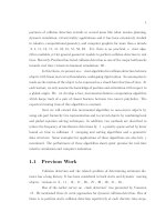
Fig. 1. Test rig.
2. System modelling
The modelling of the pneumatically driven parallel robot involves the mechanical
subsystem and the pneumatic subsystem, which are coupled by the torques resulting from
the tension forces of a pair of pneumatic muscles, respectively.
2.1 Multibody model of the parallel robot
The control-oriented multibody model of the parallel robot part consists of three rigid
bodies (Fig. 2): the two cranks as actuated links with identical properties (mass m
A
, reduced
mass moment of inertia w.r.t. the actuated axis J
A
, centre of gravity distance s
A
to the centre
of gravity, length of the link l
A
, pulley radius r) and the end-effector E (mass m
E
), which is
modelled as lumped mass.

Fig. 2. Multibody model of the parallel robot.
Nonlinear Model-Based Control of a Parallel Robot Driven by Pneumatic Muscle Actuators

27
The inertia properties of the remaining two links with length l
P
, which are designed as light-
weight construction, shall be neglected in comparison to the other links. The inertial xz-

coordinate system is chosen in the middle of the straight line that connects both base joints.
The motion of the parallel robot is completely described by two generalised coordinates q
1
(t)
and q
2
(t) that denote the two crank angles, which are combined in the vector q = [q
1
, q
2
]
T
.
Analogously, the vector of the end-effector coordinates is defined as r = [x
E
, z
E
]
T
.


Fig. 3. Ambiguity of the robot kinematics.
The direct kinematics can be stated in symbolic form and describes the vector of end-effector
coordinates r in terms of given crank angles q, i.e.

3
(, )k
=
rrq . (1)

Here, the configuration parameter k
3
is introduced to cope with two possible configurations,
see Fig. 3. The relationship between the corresponding velocities is obtained by
differentiation with respect to time

∂
==
∂
3
33
(, )
(, ) , (, )
T
k
kk
rq
rJq q Jq
q

, (2)
where J(q, k
3
) denotes the corresponding Jacobian. Here, singularities in the Jacobian can be
avoided by model-based trajectory planning. Analogously, the acceleration relationship is
given by

33
(, ) (, )kk=+rJq qJq q


  
. (3)
For a given end-effector position r the corresponding crank angles follow from the inverse
kinematics

12
(, , )kk
=
qqr , (4)
New Approaches in Automation and Robotics

28
which can be determined in symbolic form. The given ambiguity is taken into account by
introducing two configuration parameters k
1
and k
2
as shown in Fig. 3. The relationships
between the corresponding velocities as well as the accelerations follow from direct
kinematics

1
3
1
33
(, ) ,
(, )[ (, )].
k
kk
−

−
=
=−
qJ r r
qJ q rJq q


  
(5)


Fig. 4. Free-body diagram of the parallel robot.
The equations of motion for the actuated links can be directly derived from the free-body
diagram in Fig. 4 applying the principle of angular momentum

1
2
111 11 11
222 22 22
[] cos sin,
[] cos sin.
AMlMrAA EA
AMlMrAA EA
Jq rF F mgs q Fl
Jq rF F mgs q F l
βη
τ
β
η
τ

⋅=⋅ − − ⋅⋅⋅ + ⋅⋅ +
⋅=⋅ − − ⋅⋅⋅ − ⋅⋅ +




(6)
Here, the driving torque τ
i
of drive i depends on the corresponding muscle forces, i.e. τ
i
= r
[F
Mil
− F
Mir
]. At this, the indices of all variables describing a particular pneumatic muscle are
chosen as follows: the first index i = {1, 2} denotes the drive under consideration, described
by the generalised coordinate q
i
(t), whereas the second index j = {l, r} stands for the
mounting position, i.e. for the left or the right pneumatic muscle. The disturbance torque η
i

accounts for friction effects as well as remaining uncertainties in the muscle force
characteristics (13) of drive i, respectively. The coupling forces F
1E
and F
2E
are obtained from

Newton’s second law applied to the end-effector

121
122
cos cos
sin sin
()
E
EE
E
EE
F
mx
F
mgz
γγ
γγ
−
⋅
⎡⎤
⎡
⎤⎡ ⎤
=
⎢⎥
⎢
⎥⎢ ⎥
⋅+
⎣
⎦⎣ ⎦
⎣⎦



. (7)
The equations of motion in minimal form for the crank angles can be derived in two steps.
First, the last equation has to be solved for the unknown forces
Nonlinear Model-Based Control of a Parallel Robot Driven by Pneumatic Muscle Actuators

29

1
112
212
cos cos
sin sin
()
E
EE
E
EE
F
mx
F
mgz
γγ
γγ
−
−
⋅
⎡
⎤

⎡⎤⎡ ⎤
=
⎢
⎥
⎢⎥⎢ ⎥
⋅+
⎣⎦⎣ ⎦
⎣
⎦


, (8)
which then can be eliminated in (6). Second, the substitution of the variables γ
i
= γ
i
(q), β
i
=
β
i
(q), and (3) resulting from direct kinematics leads to the envisaged minimal form of the
equations of motion

() (,) () ()++=
 
Mqq kqq Gq Qq , (9)
with the mass matrix
M(q), the vector of centrifugal and Coriolis terms
(,)


kqq
and the
vector of gravity torques
G(q). The vector of generalised torques Q(q) contains the
corresponding muscle forces times the radius r of the pulley

11
22
()
M
lMr
M
lMr
FF
r
FF
−
⎡
⎤
=⋅
⎢
⎥
−
⎣
⎦
Qq
. (10)
Note that this minimal form of the equations of motions is not compulsory. Instead the
corresponding system of differential-algebraic equations can be utilised as well for the

flatness-based control design.
2.2 Modelling of the pneumatic subsystem
The parallel robot is equipped with four pneumatic muscle actuators. The contraction
lengths of the pneumatic muscles are related to the generalised coordinates, i.e. the crank
angles q
i
. The position of the crank angle, where the corresponding right pneumatic muscle
is fully contracted, is denoted by q
i0
. Consequently, by considering the transmission
consisting of toothed belt and pulley, the following constraints hold for the contraction
lengths of the muscles

0
,max 0
() ( ),
() ( ).
Mil i i i
Mir i M i i
qrqq
qrqq
Δ
=⋅ −
Δ=Δ−⋅−
A
AA
(11)
Here, ∆ℓ
M,max
is the maximum contraction given by 25% of the uncontracted length.

The volume characteristic of the pneumatic muscle (Fig. 5) can be approximated with high
accuracy by the following nonlinear function of both contraction length and muscle
pressure, where the coefficients in this polynomial approximation have been identified by
measurements

()()
31
00
(,)
mn
M
i
j
Mi
j
mMi
j
nMi
j
mn
Vp a bp
==
Δ=⋅Δ⋅⋅
∑∑
AA. (12)
The force characteristic F
Mij
(p
Mij
,∆ℓ

Mij
) of the pneumatic muscle shown in Fig. 6 describes the
resulting static tension force for given internal pressure p
Mij
as well as given contraction
length ∆ℓ
Mij
. This nonlinear force characteristic has been identified by static measurements
and, then, approximated by the following polynomial description

() ()
34
00
() ()
mn
M
i
j
Mi
j
Mi
j
Mi
j
Mi
j
Mi
j
mMi
j

Mi n Mi
j
mn
FF p f c p d
==
=Δ⋅−Δ= ⋅Δ⋅− ⋅Δ
∑∑
AAA A. (13)
New Approaches in Automation and Robotics

30

Fig. 5. Volume characteristic of a pneumatic muscle.


Fig. 6. Force characteristic of a pneumatic muscle.
The dynamics of the internal muscle pressure follows directly from a mass flow balance in
combination with the pressure-density relationship. As the maximum internal muscle
pressure is limited by a maximum value of p
max
= 7 bar, the ideal gas equation can be utilised
as accurate description of the thermodynamic behaviour of the compressed air

M
ij Mij Mij
pRT
ρ
=
⋅⋅. (14)
Here, the density ρ

Mij
, the gas constant R of air, and the thermodynamic temperature T
Mij

are introduced. For the thermodynamic process a polytropic change of state is assumed.
Thus, the relationship between the time derivative of the pressure and the time derivative of
the density results in

M
ij Mij Mij
pnRT
ρ
=
⋅⋅ ⋅

. (15)
Nonlinear Model-Based Control of a Parallel Robot Driven by Pneumatic Muscle Actuators

31
The mass flow balance for the pneumatic muscle is governed by

()
()
1
,
,
M
i
j
Mi

j
Mi
j
Mi
j
Mi
j
Mi
j
Mij Mij Mij
mVp
Vp
ρρ
⎡
⎤
=−⋅Δ
⎣
⎦
Δ


A
A
. (16)
The resulting pressure dynamics is given by a nonlinear first order differential equation and
shall not be neglected as in (Carbonell et. al., 2001)

1
Mij Mij
M

i
j
Mi
j
Mi
j
Mi
j
i
Mij
Mij i
Mij Mij
Mij
V
p
RT m p q
V
q
Vn p
p
⎡
⎤
∂∂Δ
=⋅⎢⋅⋅−⋅⋅⋅⎥
∂
∂Δ ∂
⎢
⎥
⎣
⎦

+⋅ ⋅
∂
A

A
. (17)
The internal temperature T
Mij
can be approximated with good accuracy by the constant
temperature T
0
of the ambiance (Göttert, 2004). Thereby, temperature measurements can be
avoided, and the implementational effort is significantly reduced.
3. Control design based on differential flatness
A nonlinear system in state space notation is denoted as differentially flat (Fliess et. al.,
1995), if flat outputs

()
( , , , , ), dim( ) dim( )
α
==yy uu u y u

x
(18)
exist that allow for expressing all system states
x and all system inputs u in the form

()
(1)
(,, , ),

(,, , ).
β
β
+
=
=
xxyy y
uuyy y


(19)
As a result, offline trajectory planning considering state and input constraints become
possible. Moreover, the stated parametrization of the complete system dynamics by the flat
outputs can be exploited for pure feedforward control as well as combined feedforward and
feedback control.
3.1 Flatness-based pressure control
The nonlinear state equation (17) for the internal muscle pressure p
Mij
represents the basis
for the decentralized pressure control. It can be re-formulated as

(
)
(
)
=− Δ Δ ⋅ + Δ ⋅


AA A,, ,
M

i
jp
i
j
Mi
j
Mi
j
Mi
j
Mi
j
ui
j
Mi
j
Mi
j
Mi
j
pk ppk pm
. (20)
With the internal muscle pressure as flat output candidate
y
ijp
= p
Mij
, (20) can be solved for
the mass flow
M

ij
m

as control input
u
ijp
and leads to the inverse model for the pressure
control

()
()
1
,,
,
M
i
j
i
jp
i
j
Mi
j
Mi
j
Mi
j
Mi
j
uij Mij Mij

mvkpp
kp
⎡
⎤
=⋅+ΔΔ⋅
⎣
⎦
Δ


AA
A
, (21)
New Approaches in Automation and Robotics

32
Since the internal pressure p
Mij
as state variable is identical to the flat output and dim(y
ijp
) =
dim(u
ijp
) = 1 holds, the differential flatness property is proven. The contraction length ∆ℓ
Mij

as well as its time derivative can be considered as scheduling parameters in a gain-
scheduled adaptation of
k
uij

and k
pij
. With the internal pressure as flat output, its first time
derivative is introduced as new control input

M
ij ij
p
v
=

. (22)
Consequently, the state variable of the corresponding Brunovsky form has to be provided
by means of measurements, i.e.
z
ijp
= p
Mij
. Each pneumatic muscle is equipped with a
pressure transducer mounted at the connection flange that connects the muscle with the
toothed belt. For the contraction length and its time derivative either measured or desired
values can be employed: in the given implementation, the scheduling parameter ∆
ℓ
Mij
results
from the measured crank angle
q
i
, which is obtained by an encoder providing high
resolution. Furthermore, the second scheduling parameter, the contraction velocity, is

derived from the crank angle
q
i
by means of real differentiation using a DT
1
-System with the
corresponding transfer function

1
1
()
1
DT
s
Gs
Ts
=
⋅
+
. (23)
The error dynamics of each muscle pressure
p
Mij
can be asymptotically stabilised by the
following control law which is evaluated with the measured pressure. Using this control law
all nonlinearities are compensated for. An asymptotically stable error dynamics is obtained
by pole placement

10
10

0
()
Mij ij
pij pij
ij Mijd Mijd Mij
pv
ee
vp p p
α
α
=
⎫
⎪
⇒+⋅=
⎬
=+ −
⎪
⎭



, (24)
where the constant
α
10
is determined by pole placement. Here, the desired value for the time
derivative of the internal muscle pressure can be obtained either by real differentiation of
the corresponding control input
u
ij

in (33) or by model-based calculation using only desired
values, i.e.

(,,, , )
M
ijd Mijd Mid Mid
pp pp
=
rrr

 
. (25)
The corresponding desired trajectories are obtained from a trajectory planning module that
provides synchronous time optimal trajectories according to given kinematic and dynamic
constraints (Aschemann & Hofer, 2005). It becomes obvious that a continuous time
derivative
M
ijd
p

requires a three times continuously differentiable desired end-effector
trajectory r.
The implementation of the underlying flatness-based pressure control structure for drive i is
depicted in Fig. 7. In each input channel, the nonlinear valve characteristic (VC) is
compensated by pre-multiplying with its approximated inverse valve characteristic (IVC).
This inverse valve characteristic is implemented as look-up-table and depends both on the
commanded mass flow and on the measured internal pressure.
Nonlinear Model-Based Control of a Parallel Robot Driven by Pneumatic Muscle Actuators

33

Fig. 7. Implementation of the underlying pressure control structure for drive i.
3.2 Inverse dynamics of the decoupling control
For the outer control loop design the generalised coordinates and the mean muscle
pressures are chosen as flat output candidates

1
1
2
2
11
1
222
(, )
2
2
M
lMr
M
M
Ml Mr
q
q
q
q
pp
p
ppp
⎡
⎤

⎢
⎥
⎡⎤
⎢
⎥
⎢⎥
⎢
⎥
+
⎢⎥
== =
⎢
⎥
⎢⎥
⎢
⎥
⎢⎥
+
⎢
⎥
⎢⎥
⎣⎦
⎢
⎥
⎣
⎦
yyxu
, (26)
where the input vector u contains the four muscle pressures

11 22
T
Ml Mr Ml Mr
pppp=
⎡
⎤
⎣
⎦
u
(27)
and the state vector
x consists of the vector of generalised coordinates q as well as their time
derivatives
q



⎡
⎤
=
⎢
⎥
⎣
⎦
q
x
q

. (28)
The trajectory control of the mean pressure allows for increasing stiffness concerning

disturbance forces acting on the end-effector (Bindel et. al., 1999). As the decentralised
pressure controls have been assigned a high bandwidth, these four controlled muscle
New Approaches in Automation and Robotics

34
pressures p
Mij
can be considered as ideal control inputs of the outer control loop. Subsequent
differentiation of the first two flat output candidates until one of the control appears leads to


11
11
11 1 1
,
,
(,, , ),
M
lMr
yq
yq
yq p p
=
=
= qq


 
(29)
and

22
22
22 2 2
,
,
(,, , ),
Ml Mr
yq
yq
yq p p
=
=
= qq


 
(30)

whereas the third and fourth flat output candidates directly depend on the control inputs

31 1 1
42 2 2
0.5 ( ),
0.5 ( ).
M
Ml Mr
M
Ml Mr
yp p p

yp p p
=
=⋅ +
==⋅ +
(31)
The differential flatness can be proven as follows: all system states can be directly expressed
by the flat outputs and their time derivatives

1212
T
yyyy
⎡⎤
==
⎡
⎤
⎢⎥
⎣
⎦
⎣⎦
q
x
q


. (32)
The equations of motion (9) are available in symbolic form. Inserting the muscle force
characteristics, the internal muscle pressures as control inputs can be parameterized by the
flat outputs and their time derivatives

11

11
12
22
22
(,,, )
(,,, )
(,,, , )
(,,, )
(,,, )
Ml M
Mr M
MM
Ml M
Mr M
pp
pp
pp
pp
pp
⎡⎤
⎢⎥
⎢⎥
==
⎢⎥
⎢⎥
⎢⎥
⎣⎦
qqq
qqq
uuqqq

qqq
qqq





. (33)
In the following, three different nonlinear control approaches are employed to stabilize the
error dynamics of the outer control loop: flatness-based control, backstepping and sliding-
mode control (Khalil, 1996). For all these alternative designs, the differential flatness
property proves advantageous (Sira-Ramirez & Llanes-Santiago, 1995; Aschemann et. al.,
2007).
3.3 Flatness-based control
In the case of flatness-based control, the inverse dynamics is evaluated with the measured
crank angles and the corresponding angular velocities obtained by real differentiation
(Aschemann & Hofer, 2005). For the mean pressures, however, desired values are utilized.
The second derivatives of the crank angles, the angular accelerations, serve as stabilizing
inputs

11 22 1212
(,, , , , )
T
M
lMrMlMr MdMd
pppp vvpp==
⎡⎤
⎣⎦
uuqq


. (34)

The inverse dynamics leads to a compensation of all nonlinearities. An asymptotic
stabilization is achieved by pole placement with Hurwitz-polynomials for the error
dynamics for each drive i = {1, 2}
Nonlinear Model-Based Control of a Parallel Robot Driven by Pneumatic Muscle Actuators

35

21 0
0
()() ()
t
i id i id i i id i i id i
vq qq qq qqd
α
αατ
=+⋅ −+⋅ −+ ⋅ −
∫
  
. (35)
3.4 Backstepping control
The first step of the backstepping control design (Khalil, 1996) involves the definition of the
tracking error variable for each drive i = {1, 2},

11iidi iidi
eqq eqq
=
−⇒ =−


. (36)
Next, a first Lyapunov function V
i1
is introduced

!
22
11 1 11 1 1 1 1 1
1
() 0 () ( )
2
ii i i i i i id i i
Ve e Ve e e e q q ce
=
>⇒ =⋅=⋅ −=−⋅


(37)
and the expression for its time derivative is solved for the virtual control input

111 111
(,)
iidi i iiIiidid i
eqq ce q eq qce
α
=
−=−⋅ ⇒ ≈ = +⋅
   
. (38)
In the second step, the error variable e

i2
is defined in the following form

21 11 1211
(,)
iiIiidiidi i ii i
eeqqqqce eece
α
=
−= −+⋅ ⇒ = −⋅
 
(39)
and its time derivative is computed

2111211
()
iidi iidi i i
eqqceqqcece
=
−+⋅ = −+⋅ −⋅
 
. (40)
Now, a second Lyapunov function V
i2
is specified.

22
212 1 2 212 1 1 2 2
11
(,) 0 (,)

22
iii i i iii i i i i
Vee e e Vee e e e e
=
+>⇒ =⋅+⋅


(41)
The corresponding time derivative

!
222
212 1 1 2 1 2 1 1 1 1 1 2 2
(,) [ ( ) ]
iii iiidi i i i i i
Vee ce e q v c e ce e ce ce
=
−⋅ + ⋅ − + ⋅ − ⋅ + =− ⋅ − ⋅


(42)
can be made negative definite by choosing the stabilizing control input as follows

2
11212
(1 ) ( )
iiidi i
v
qq
ececc== + ⋅− + ⋅ +

 
. (43)
Backstepping control design offers several advantages in comparison to flatness based
control. It becomes possible to avoid cancellations of useful, i.e. stabilizing nonlinearities.
Furthermore, different positive definite functions can be used at control design, e.g.
allowing for nonlinear damping.
3.5 Sliding-mode control
For sliding-mode control (Sira-Ramirez & Llanes-Santiago, 1995) the vector of tracking
errors is considered


id i
i
id i
qq
qq
−
⎡
⎤
=
⎢
⎥
−
⎣
⎦
z

. (44)
New Approaches in Automation and Robotics

36
Based on this error vector z
i
, the following sliding surfaces s
i
are defined for each drive
i = {1, 2}

11
() () ()
i i id i i id i i id i i id i
sqqqqsqqqq
β
β
=
−+ ⋅ − ⇒ = −+ ⋅ −z
  
, (45)
where
β
i1
represents a positive gain. The convergence to the corresponding sliding surface is
achieved by introducing a discontinuous switching function in the time derivative of a
quadratic Lyapunov function

2
1
() () || ()
2
ii i ii i i i i i i i

Vs s Vs s s s s signs
αα
=⇒ =⋅≤−=−⋅⋅


, (46)
with a properly chosen coefficient
α
i
that dominates remaining model uncertainties. The
control design offers flexibility as regards the choice of the sliding surfaces and the reaching
laws. For the implementation, however, a smooth switching function is preferred to reduce
high frequency chattering. This results in the following stabilizing control law, which leads
to a real sliding mode within a boundary layer

1
()tanh()
i
iiidi idi i
s
vqq q q
βα
ε
== + ⋅ − +⋅
   
. (47)
The implemented control structure is depicted in Fig. 8. The desired trajectories are
provided from an offline trajectory planning module that calculates time optimal trajec-
tories according to both state constraints and input constraints. This is achieved by proper
time-scaling of polynomial functions with free parameters as described in (Aschemann &

Hofer, 2005).


Fig. 8. Implementation of the decoupling control structure.
4. Disturbance observer design
The observer provides a vector
2
ˆ
x of estimated disturbance torques that accounts for both
model uncertainties and nonlinear friction. The main idea consists in the extension of the
system state equations with the measurable state vector
Nonlinear Model-Based Control of a Parallel Robot Driven by Pneumatic Muscle Actuators

37

1
[,]
T
==yx qq

(48)
by two integrators, which serve as disturbance models (Aschemann et. al., 2007)

2
22
ˆ
(, ,), dim() 4,
ˆˆ
,dim( )2.
=

=
==
yfyxu y
x0 x


(49)
The reduced-order disturbance observer according to (Friedland, 1996) is given by

η
η
=
Φ=
⎡⎤
==+
⎢⎥
⎣⎦
2
1
2
2
ˆ
(, ,), dim() 2,
ˆ
ˆ
,
ˆ
zyxu z
xHyz


(50)
where H denotes the observer gain matrix and z the observer state vector. The observer gain
matrix is chosen as follows

11 11
22 22
00
00
hh
hh
⎡
⎤
=
⎢
⎥
⎣
⎦
H
, (51)
involving only two design parameters h
11
and h
22
. Aiming at an asymptotically stable
observer dynamics

!
22
ˆ
lim lim( )

tt→∞ →∞
=
−=exx0, (52)
the observer gains are determined by pole placement based on a linearization using the
corresponding Jacobian (Friedland, 1996). In Fig. 9 a comparison of simulated disturbance
forces and the observed forces provided by the proposed disturbance observer is shown.
Here, the resulting tangential force at the pulley with radius r is depicted, which is related to
the disturbance torque according to
η
=
ˆ
/
iU i
Fr. Obviously, the simulated disturbance
forces are reconstructed with high accuracy.

0 5 10 15
-100
-50
0
50
100
t [s]
tangential force [N]
0 5 10 15
-100
-50
0
50
100

t [s]
tangential force [N]
actual disturbance F
1U
observed F
1U
actual disturbance F
2U
observed F
2U

Fig. 9. Comparison of simulated disturbance force and observed disturbance force using the
reduced-order disturbance observer.
New Approaches in Automation and Robotics

38
5. Simulation results
The efficiency of the proposed cascade control structure is investigated using the desired
trajectory shown in Fig. 10 with maximum velocities of approx. 0.9 m/s and maximum
accelerations of approx. 7 m/s
2
for each axis.
The first part of the desired trajectory involves the motion on a quarter-circle with the radius
0.2 m from the starting point (x = 0 m, z = 1 m) to the point (x = −0.2 m, z = 0.8 m). The next
three movements consist of straight lines: the second part comprises a diagonal movement
in the xz-plane to the point (x = −0.1 m, z = 0.6 m), followed by a straight line motion in x-
direction to the point (x = 0.1 m, z = 0.6 m). The fourth part is given by a diagonal movement
to the point (x = 0.2 m, z = 0.8 m). The fifth part involves the return motion on a quarter-
circle to the starting point (x = 0 m, z = 1 m).

Fig. 10. Desired trajectory in the workspace.

0 5 10 15
-5
0
5
x 10
-3
t [s]
e
x
[m]
BS
BS
FB
SM
0 5 10 15
-15
-10
-5
0
5
x 10
-3
t [s]
e
z
[m]
BS

FB
SM

Fig. 11. Comparison of the tracking errors in the workspace without disturbance observer.
Nonlinear Model-Based Control of a Parallel Robot Driven by Pneumatic Muscle Actuators

39
Fig. 11 shows a comparison of the resulting tracking errors in the workspace for flatness-
based control (FB), backstepping control (BS) and sliding-mode control (SM). Without
observer-based disturbance compensation, the best results are obtained using sliding-mode
control.
The efficiency of the observer based disturbance compensation is emphasized by Fig. 12. For
all considered control approaches a further improvement of tracking accuracy is achieved.
6. Conclusion
In this contribution, a cascaded trajectory control based on differential flatness is presented
for a parallel robot with two degrees of freedom driven by pneumatic muscles. The
modelling of this mechatronic system leads to a system of nonlinear differential equations of
eighth order. For the characteristics of the pneumatic muscles polynomials serve as good
approximations. The inner control loops of the cascade involve a flatness-based control of
the internal muscle pressure with high bandwidth. For the outer control loop three different
control approaches have been investigated leading to a decoupling of the crank angles and
the mean pressures as controlled variables. Simulation results emphasize the excellent
closed-loop performance with maximum position errors of approx. 1 mm during the
movements, vanishing steady-state position error and steady-state pressure error of less
than 0.03 bar, which have been confirmed by first experimental results at a prototype
system.

0 5 10 15
-1
-0.5

0
0.5
1
x 10
-3
t [s]
e
x
[m]
BS
FB
SM
0 5 10 15
-1
-0.5
0
0.5
1
1.5
x 10
-3
t [s]
e
z
[m]
BS
FB
SM

Fig. 12. Tracking errors in the workspace with observer-based disturbance compensation.

7. References
Aschemann H.; Hofer E.P. (2004). Flatness-Based Trajectory Control of a Pneumatically Driven
Carriage with Uncertainties, CD-ROM-Proc. of NOLCOS, pp. 239 – 244, Stuttgart,
September 2004
Aschemann H.; Hofer E.P. (2005). Flatness-Based Trajectory Planning and Control of a Parallel
Robot Actuated by Pneumatic Muscles, CD-ROM-Proc. of the ECCOMAS Thematic
Conference on Multibody Dynamics, Madrid, June 2005
Aschemann H.; Knestel, M.; Hofer E.P. (2007). Nonlinear Control Strategies for a Parallel Robot
Driven by Pneumatic Muscles, Proc. of 14
th
Int. Workshop on Dynamics and Control,
Moscow, June 2007, Nauka, Moscow
New Approaches in Automation and Robotics

40
Bindel, R.; Nitsche, R.; Rothfuß, R.; Zeitz, M. (1999). Flatness Based Control of Two Valve
Hydraulic Joint Actuator of a Large Manipulator. CD-ROM-Proc. of ECC, Karlsruhe,
1999
Carbonell P.; Jian Z.P.; Repperger D. (2001). Comparative Study of Three Nonlinear Control
Strategies for a Pneumatic Muscle Actuator, CD-Proc. of NOLCOS, Saint-Petersburg,
pp. 167 – 172, June 2001
Fliess M.; Levine J.; Martin P.; Rouchon P. (1995). Flatness and Defect of Nonlinear Systems:
Introductory Theory and Examples, Int. J. of Control, Vol. 61, No. 6, pp. 1327 – 1361
Friedland, B. (1996). Advanced Control System Design, Prentice-Hall
Göttert, M. (2004). Bahnregelung servopneumatischer Antriebe, Berichte aus der Steuerungs-
und Regelungstechnik (in German), Shaker
Khalil, H. K. (1996). Nonlinear Systems, 2nd. ed., Prentice-Hall
Sira-Ramirez H.; Llanes-Santiago O. (1995) Sliding Mode Control of Nonlinear Mechanical
Vibrations, J. of Dyn. Systems, Meas. and Control, Vol. 122, No. 12, pp. 674 – 678

3
Neural-Based Navigation Approach
for a Bi-Steerable Mobile Robot
Azouaoui Ouahiba, Ouadah Noureddine,
Aouana Salem and Chabi Djeffer
Centre de Développement des technologies Avancées (CDTA)
Algeria
1. Introduction
Recent developments in robotics have revealed a strong demand for autonomous out-door
vehicles capable of some degree of self-sufficiency. These vehicles have many applications in
a large variety of domains, from spatial exploration to handling material, and from military
tasks to people transportation (Azouaoui &Chohra, 1998; Hong et al., 2002; Kujawski, 1995;
Labakhua et al., 2006; Niegel, 1995; Schafer, 2005; Schilling & Jungius, 1995; Wagner, 2006).
Most mobile robot missions include autonomous navigation. Thus, vehicle designers search
to create dynamic systems able to navigate and achieve intelligent behaviors like human in
real dynamic environments where conditions are laborious.
In this context, these last few years small automated and non-pollutant vehicles are
developed to perform a public urban transportation task. These vehicles must use advanced
control techniques for navigation in dynamic environments especially urban ones. Indeed,
several research works have recently emerged to treat this transportation task problem. For
instance, the work developed in (Gu & Hu, 2002) presents a path-tracking scheme based on
wavelet neural predictive control to model non-linear kinematics of the robot to adapt it to a
large operating range. In (Mendes et al., 2003), a path-tracking controller with an anti-
collision behavior of a car-like robot is presented. It is based on navigation and anti-collision
systems. The first system uses a Fuzzy Logic (FL) to implement the path-tracking while the
second system consists of estimating the trajectories and behavior of surrounding objects.
Another work developed in (Bento & Nunes, 2004) treats also the path following problem of
a cybernetic car. The developed controller with magnetic markers guidance is based on FL
and integrates an anti-collision behavior applied to a bi-steerable vehicle. Other works use a
visual control to achieve a desired task such as the work proposed in (Avina Cervantes,

2005). It consists to develop a visual-based navigation method for mobile robots using an
on-board color camera. The objective is the use of vehicles in agriculture to navigate
automatically on a network of roads (to go from a farm to a given field for example).
Although several investigations on the robot navigation problem have been developed
(Avina Cervantes, 2005; Azouaoui & Chohra, 2002; Chohra et al., 1998; Gu & Hu, 2002;
Kujawski, 1995; Labakhua et al., 2006; Mendes et al., 2003; Niegel, 1995; Schilling & Jungius,
1995; Sorouchyari, 1989), to date further efforts must be made to apprehend and understand
New Approaches in Automation and Robotics

42
the navigation behavior of a vehicle evolving in partially structured and partially known
environments such as urban ones.
In this paper, an interesting neural-based navigation approach suggested in (Azouaoui &
Chohra, 2002; Chohra et al., 1998) is applied with some modifications to a bi-steerable
mobile robot Robucar. Indeed, this approach is based on basic behaviors which are fused
under a neural paradigm using Gradient Back-Propagation (GBP) learning algorithm. This
navigation is then implemented within a behavioral architecture because of its excellent
real-time execution properties (Murphy, 2001).
The aim of this work is to implement a neural-based navigation approach able to provide
the Robucar with more autonomy, intelligence, and real-time processing capabilities. In fact,
the vehicle relies on its interaction with its environment to extract useful information. In this
paper, the used neural navigation approach essentially based on pattern classification (or
recognition) (Welstead, 1994) of target localization and obstacle avoidance behaviors is
presented. This approach has been developed in (Chohra et al., 1998) for five (05) possible
movements of vehicles, while in this paper this number is reduced to three (03) possible
movements due to the Robucar structure. Second, simulation results of the neural-based
navigation are presented. Finally, an implementation of the neural-based navigation on a
real bi-steerable robot Robucar is given leading to a learning vehicle able to behave
intelligently faced to unexpected situations.
2. Neural-based navigation approach applied to a bi-steerable mobile robot

Robucar in partially structured environnments
To navigate in partially structured environments, the Robucar must reach its target without
collisions with possibly encountered obstacles. In other terms, it must have the capability to
achieve the target localization, obstacle avoidance, and decision-making and action
behaviors. These behaviors are acquired using multilayer feedforward Neural Networks
(NN).
This neural navigation is built of three (03) phases as shown in Figure 1. During the phase 1,
from the temperature field vector X
T
, the robot learns to recognize target location situations
T
j1
(j1 = 1, , 5) classifier while it learns to recognize obstacle avoidance situations O
j2
(j2 = 1,
, 6) classifier from the distance vector X
O
during the phase 2. The phase 3 decides an action
A
i
(i = 1, , 3) from two (02) association stages and their coordination carried out by
reinforcement Trial and Error learning.

Obstacle Avoidance
(NN2 Classifier)
Target Localization
(NN1 Classifier)
PHASE2
PHASE3
PHASE1

O
T
X
O
XT
A
Decision-Makin
g
and Action (NN3)
Coordination
Association
Association

Fig. 1. Neural navigation system synopsis.
Neural-Based Navigation Approach for a Bi-Steerable Mobile Robot

43
2.1 Vehicule and sensor
a) Vehicle.
The Robucar is a non-holonomic robot characterized by its bounded steering angle (-18°≤ φ≤
+18°) and velocity (0m/s ≤v ≤5m/s) (Figure 2(a)). Three movements of the Robucar are
defined to ensure safety displacement in the environment. The possible movements are then
in three (03) directions consequently three (03) possible actions are defined as action to move
left (towards 18°), action to move forward (towards 0°), and action to move right (towards -
18°) as shown in Figure 2(b). They are expressed by the action vector A = [A
1
, A
2
, A
3

].

(a) Robucar. (b) Robot model.
Fig. 2. Robucar and its sensor.
b) Sensor.
The perception system is essentially based on a laser-range finder LMS200 ( SICK, 2001). It
provides either 100° or 180° coverage with 0.25°, 0.5°, or 1.0° angular resolution. In this
paper, the overall coverage area is divided into three sub-areas corresponding to the three
possible actions as shown in Figure 2. Thus, to detect possibly encountered obstacles, three
(03) areas are defined to get distances (vehicle-obstacle) from 45° to 81°, from 81° to 99°, and
from 99° to 135° ( see Figure 2). These areas are deduced from the Robucar dimensions to
ensure its security.
2.2 Neural-based navigation system
During the navigation, the vehicle must build an implicit internal map (i.e., target, obstacles,
and free spaces) allowing recognition of both target location and obstacle avoidance
situations. Then, it decides the appropriate action from two association stages and their
coordination (Chohra et al., 1998; Sorouchyari, 1989). To achieve this, the neural-based
navigation system is used where the only known data are initial and final (i.e., target)
positions of the vehicle.
a) Phase 1.
Target Localization (NN1 Classifier). The target localization behavior is based on NN1
classifier trained by the GBP algorithm which must recognize five (05) target location
situations, after learning, from data obtained by computing distance and orientation of
45°
99°
A
2
A
1 A
3

M
Robucar
135°
270°
81°
New Approaches in Automation and Robotics

44
robot-target using a temperature field method (Sorouchyari, 1989). This method leads to
model the vehicle environment in five (05) areas corresponding to all target locations as
shown in Figure 3. These situations are defined with five (05) Classes T
1
, , T
j1
, , T
5
where
(j1 = 1, , 5):
If 45° ≤ γ < 81° (Class T
1
),
If 81° ≤ γ < 99° (Class T
2
),
If 99° ≤ γ < 135° (Class T
3
),
If 135° ≤ γ < 270° (Class T
4
),

If 270° ≤ γ < 405° (Class T
5
). (1)
where γ is the angle of the target direction.


Fig. 3. Target location situations.
Temperatures in the neighborhood of the vehicle are defined by: t
L
in direction 18°, t
F
in
direction 0°, and t
R
in direction -18°. These temperatures are computed using sine and cosine
functions as follows:

If 45°< γ≤80° (Class T
1
),
Then T
R
= 12sin (γ), T
F
= 6cos (γ), T
L
= 6cos (γ),
If 80°< γ≤99° (Class T
2
),

Then T
R
= 6|cos (γ)|,T
F
= 12sin (γ),T
L
= 6|cos (γ)|,
If 99°< γ≤135° (Class T
3
),
Then T
R
= 6|cos (γ)|,T
F
= 6|sin (γ)|,T
L
= 12sin(γ),
If 135°< γ≤270° (Class T
4
),
Then T
R
= 12|sin (γ)|,T
F
= 6|sin (γ)|,T
L
= 12|sin(γ)|,
If 270°< γ≤315° (Class T
5
),

Then T
R
= 12|sin (γ)|,T
F
= 6|sin (γ)|,T
L
= 6cos(γ),
If 315°< γ≤360° (Class T
5
),
Then T
R
= 12cos (γ),T
F
= 6cos (γ),T
L
= 6|sin(γ)|,
If 360°< γ≤405° (Class T
5
),
Then T
R
= 12cos (γ),T
F
= 6cos (γ), T
L
= 6sin(γ). (2)
270°
99°
A

2
A
1
A
3
T
4
T
5

T
3
M
Robuca
r
135°
T
1
81°
T
2
45°

Neural-Based Navigation Approach for a Bi-Steerable Mobile Robot

45
These components are pre-processed to constitute the input vector X
T
of NN1 (Azouaoui &
Chohra, 2003; Azouaoui & Chohra, 2002; Chohra et al., 1998) built of input layer, hidden

layer, and output layer as shown in Figure 4: architecture of NN1 where X
i
= X
Ti
(i = 1, , 3),
Y
k
(k = 1, , 5), C
j
= T
j1
(j = j1 = 1, , 5).


i
k
j
Y
k
X
i

W2
ki

W1
jk
Output Layer
Hidden Layer
Input Layer

Desired
C
j










C
j



Fig. 4. Architecture of both NN1 and NN2.
After learning, for each input vector X

T
, NN1 provides the vehicle with capability to decide
its target localization, recognizing target location situation expressed by the highly activated
output T
j1
.
b) Phase 2.
Obstacle Avoidance (NN2 Classifier). The obstacle avoidance behavior is based on NN2
classifier trained by GBP which must recognize obstacle avoidance situations, after learning,
from laser sensor data giving robot-obstacle distances. These obstacle avoidance situations
are modeled as the human perceives them, that is, as topological situations: corridors,
rooms, right turns, etc. ( Anderson, 1995; Azouaoui & Chohra, 2003).
The possible movements of the Robucar lead us to structure possibly encountered obstacles
in six (06) topological situations as shown in Figure 5. These situations are defined with six
(06) Classes O
1
, , O
j2
, , O
6
where (j2 = 1, , 6).
The robot-obstacle minimal distances are defined in the vehicle neighborhood by: d
L
in
direction 18°, d
F
in direction 0°, and d
R
in direction -18° as shown in Figure 6. These
components are pre-processed to constitute the input vector X

O
of NN2 built of input layer,
hidden layer, and output layer as shown in Figure 4: architecture of NN2 where X
i
= X
Oi
(i =
1, , 3), Y
k
(k = 1, , 6), C
j
= O
j2
(j = j2 = 1, , 6).
New Approaches in Automation and Robotics

46

Fig. 5. Obstacle avoidance situations.
After learning, for each input vector X
O
, NN2 provides the vehicle with capability to decide
its obstacle avoidance, recognizing obstacle avoidance situation expressed by the highly
activated output O
j2
.


Fig. 6. Laser range areas for obstacle detection.
c) Phase 3.

Decision-Making and Action (NN3). Two (02) association stages between each behavior
(target localization and obstacle avoidance) and the favorable actions (among possible
actions), and the coordination of these association stages are carried out by NN3. Thus, both
situations T
j1
and O
j2
are associated by the reinforcement trial and error learning with the
favorable actions separately as suggested in (Sorouchyari, 1989). Afterwards, the
coordination of the two (02) associated stages allows the decision-making of the appropriate
action.
NN3 is built of two layers (input layer and output layer) illustrated in Figure 7.
O
1
O
3
-18°
0°
+18°
O
4

O
5

O
6


-18° +18°

0° -18°
+18°
0°
O
2
81°
99°
LMS
45°
135°
d
L
Robucar
d
F
d
R
0°
180°
Neural-Based Navigation Approach for a Bi-Steerable Mobile Robot

47
1) Input Layer.
This layer is the input layer with eleven (11) input nodes receiving the components of T
j1

and O
j2
vectors. This layer transmits these inputs to all nodes of the next layer. Each node T
j1

is connected to all nodes A
i
with the connection weights U
ij1
and each node O
j2
is connected
to all nodes A
i
with the connection weights V
ij2
as shown in Figure 7.
2) Output Layer.
This layer is the output layer with three (03) output nodes which are obtained by adding the
contribution of each behavior. The Robucar learns through trial and error interactions with
the environment. It learns a given behavior by being told how well or how badly it is
performing as it acts in each given situation. As feedback, it receives a single information
item from the environment. The feedback is interpreted as positive or negative scalar
reinforcement. The goal of the learning system is to maximize positive reinforcement
(reward) and/or minimize negative reinforcement (punishment) over time (Sorouchyari,
1989; Sutton & Barto, 1998). By successive trials and/or errors, the Robucar determines a
mapping function (see figure 8) which is used for its navigation. The two association stages
are obtained as developed in (Chohra et al., 1998).
After learning, NN3 provides the vehicle with capability to decide the appropriate action
expressed by the highly activated output A
i
.
3. Simulation results
In this section, at first the training processes of NN1, NN2, and NN3 are described. Second,

the simulated neural-based navigation is described and simulation results are presented.


j1
Output Layer
Input Layer
T
1

T
5

T
j1

j2
O
1
O
6

O
j2
i
U
ij1

V
ij2

A
1
with i = 1, , 3
j1 = 1, , 5
j2 = 1, , 6.
A
3

A
i



Fig. 7. Architecture of NN3.