New Developments in Robotics, Automation and Control 2009 Part 9 pptx

Intelligent Detection of Bad Credit Card Accounts

233
were bad accounts, 1,000 (33.33%) were charge-off accounts, and 1,000 (33.33%) were normal
accounts.

Input variables that deal with cardholder’s accounts were divided into two groups:
(1) socio-economic data and (2) financial data. Basic socio-economic characteristics that are
used in our raw database are: (1) gender, (2) marital status, (3) education, (4) age and (5)
occupation. Basic financial characteristics that are used in our raw database are: (1) credit
limit, (2) current balance, (3) payment amount, (4) transaction amount, (5) revolving credit
amount, (6) late charge fee, (7) credit cash amount, (8) delinquency flag, (9) cycle, (10)
client’s account age and (11) zip code.

Clients’ accounts are classified as being either normal, bad debt, or charge-off. Clients
are in bad debt if they exceed a contracted overdraft for more than 30 days during a period
of 6 months. Clients are charge-off if they exceed a contracted overdraft for more than 180
days during a period of 6 months. Otherwise, a client is considered normal.

4.2 Data Selection
The scheme employed herein incorporates the following features: (1) Credit limit, the
maximum amount a person is allowed to borrow on a credit card (see Table 1). It includes
purchases, cash advances, and any finance charges or fees. Some issuers increase
cardholder’s credit limit to promote their consumption. Most of the bad account’s credit
limit is below NT$100,000. The normal account’s credit limit is between NT$100,000 and
NT$300,000. (2) Gender, Table 2 shows the credit status related to gender. Female clients
have a higher rate of normal accounts than male clients. Males therefore have higher risk of
bad accounts than females. (3) Education, Table 3 shows the cardholder’s education. Clients
with good education have higher rate of normal accounts than other groups. Accounts with
just a high-school diploma are at higher risk than others. (4) Marital status, the data revealed
that the credit status has no apparent relationship to marital status. (5) Cycle, a monthly

billing date from a creditor which summarizes the activity and expenses on an account
between the last billing date and the current billing date. The effect of cycle on credit status
shows no apparent difference in the entire classes as given in Table 3. (6) Age, there is a
group of high-risk cardholders between 20-40 years of age as shown in Table 4. Note that
workers younger than 20 years old or elder than 65 years old who are unemployed are
discarded (see Table 4). (7) Client account age, clients who have had accounts for about one
year make up a group of high-risk cardholders. Normal account holders continue using
their credit cards without problems beyond the first year as shown in Table 5. (8) Current
balance, the total amount of money owed on a credit line. It includes any unpaid balance
from the previous months, new purchases, cash advances and any charges at present. There
are 91.78% normal accounts owed below NT$100,000 dollars as given in Table 6. (9) Payment
amount paid before the next billing date, the bad accounts and charge-off accounts have low
payment amounts. They have no ability to pay off their credit amount as shown in Table 6.
(10) Transaction amount, the amount that a person charges and owes on a credit card between
the last billing date and the current billing date. It includes purchases, cash advances, and
any finance charges or fees. The account of poor credit status will be limited their purchase
as shown in Table 7. (11) Delinquent flag, a credit line or loan account where the late
payments have been received or the payments have not been made according to the
New Developments in Robotics, Automation and Control

234
respective terms and conditions in a current month. The charge-off account has the current
delinquent flag of long term as demonstrated in Table 8. (12) Balance to credit line ratio (B/C),
is used to record the cardholder usage of the credit line. The normal accounts use the credit
card in a good manner. The charge-off accounts have a high B/C ratio with over purchase as
shown in Table 9.

Normal account Bad debt account Charge-off account Total account
Credit limit No. % No. % No. % No. %
1 - 100000 66,090 15.2% 6,217 61.5% 3,176 61.2% 75,483 16.8%

100,001-200,000 117,227 27.0% 2,179 21.6% 1,186 22.9% 120,592 26.9%
200,001- 300,000 135,965 31.3% 1,230 12.2% 682 13.1% 137,877 30.7%
300,001- 400,000 70,572 16.3% 328 3.3% 119 2.3% 71,019 15.8%
400,001- 500,000 26,495 6.1% 124 1.2% 20 0.4% 26,639 5.9%
500,001and over 17,567 4.1% 27 0.3% 7 0.1% 17,601 3.9%
Total 433,916 100.0% 10,105 100.0% 5,190 100.0% 449,211 100.0%
Table 1. Risk related to credit limit.

Normal account Bad debt account Charge-off account Total account
Gender No. % No. % No. % No. %
Female 291,118 67.1% 4,841 47.9% 2259 43.5% 298,218 66.4%
Male 142,798 32.9% 5,264 52.1% 2931 56.5% 150,993 33.6%
Total 433,916 100.0% 10,105 100.0% 5190 100.0% 449,211 100.0%
Table 2. Risk related to gender.

Normal account Bad debt account Charge-off account Total account
Education No. % No. % No. % No. %
Master 19,725 4.6% 135 1.3% 27 0.5% 19,887 4.4%
College 193,883 44.7% 2,250 22.3% 843 16.2% 196,976 43.9%
High school 143,807 33.1% 5,302 52.5% 2,953 56.9% 152,062 33.9%
Unknown 76,501 17.6% 2,418 23.9% 1,367 26.3% 80,286 17.9%
Total 433,916 100.0% 10,105 100.0% 5,190 100.0% 449,211 100.0%
Table 3. Risk related to education.

Normal account Bad debt account Charge-off account Total account
Age No. % No. % No. % No. %
20-30 86,977 20.0% 3,071 30.4% 1,267 24.4% 91,315 20.3%
31-40 156,391 36.0% 2,976 29.5% 1,617 31.2% 160,984 35.8%
41-50 119,563 27.6% 2,550 25.2% 1,506 29.0% 123,619 27.5%
51-60 55,934 12.9% 1,275 12.6% 678 13.1% 57,887 12.9%

Intelligent Detection of Bad Credit Card Accounts

235
Normal account Bad debt account Charge-off account Total account
Age No. % No. % No. % No. %
61-70 12,302 2.8% 219 2.2% 112 2.2% 12,633 2.8%
71-80 2,713 0.6% 14 0.1% 10 0.2% 2,737 0.6%
81-90 33 0.0% 0 0.0% 0 0.0% 33 0.0%
90 and over 3 0.0% 0 0.0% 0 0.0% 3 0.0%
Total 433,916 100.0% 10,105 100.0% 5,190 100.0% 449,211 100.0%
Table 4. Comparison of credit status by age.

Normal account Bad debt account Charge-off account Total account
Account age No. % No. % No. % No. %
1 22,971 5.3% 405 4.0% 0 0.0% 23,376 5.2%
2 80,839 18.6% 3,854 38.1% 1,689 32.5% 86,382 19.2%
3 90,434 20.8% 2,276 22.5% 1,405 27.1% 94,115 21.0%
4 186,869 43.1% 2,946 29.2% 1,697 32.7% 191,512 42.6%
5 8,368 1.9% 132 1.3% 119 2.3% 8,619 1.9%
6 15,056 3.5% 164 1.6% 101 2.0% 15,321 3.4%
7 11,729 2.7% 136 1.4% 66 1.3% 11,931 2.7%
8 7,501 1.7% 79 0.8% 47 0.9% 7,627 1.7%
9 3,317 0.8% 45 0.5% 22 0.4% 3,384 0.8%
10 1,916 0.4% 19 0.2% 19 0.4% 1,954 0.4%
11 1,824 0.4% 21 0.2% 17 0.3% 1,862 0.4%
12 2,960 0.7% 28 0.3% 7 0.1% 2,995 0.7%
13 132 0.0% 0 0.0% 1 0.0% 133 0.0%
Total 433,916 100.0% 10,105 100.0% 5,190 100.0% 449,211 100.0%
Table 5. Risk related to account age.

Normal account Bad debt account Charge-off account Total account
Current Balance No. % No. % No. % No. %
0 178,493 41.1% 2,406 23.8% 11 0.2% 180,910 40.3%
1 – 100,000 219,727 50.6% 5,568 55.1% 3,374 65.0% 228,669 50.9%
100,001-200,000 22,769 5.3% 1,151 11.4% 1,046 20.2% 24,966 5.6%
200,001-
300,000
8,684 2.0% 643 6.4% 560 10.8% 9,887 2.2%
300,001-
400,000
3,005 0.7% 212 2.1% 136 2.6% 3,353 0.8%
400,001-
500,000
981 0.2% 70 0.7% 43 0.8% 1,094 0.2%
500,001-
600,000
193 0.0% 41 0.4% 9 0.8% 243 0.1%
600,001-
700,000
26 0.0% 5 0.1% 9 0.8% 40 0.0%
Total 433,916 100.0% 10,105 100.0% 5,190 100.0% 449,211 100.0%
Table 6. Risk related to current balance.
New Developments in Robotics, Automation and Control

236
Normal account Bad debt account Charge-off account Total account
Payment amount No. Percentage No. Percentage No. Percentage No. Percentage
0 334,814 77.2% 9,546 94.5% 5,104 98.3% 349,464 77.8%
1 – 100,000 64,254 14.8% 466 4.6% 75 1.5% 64,795 14.4%
100,001- 200,000 15,023 3.5% 37 0.4% 4 0.1% 15,064 3.4%

200,001- 300,000 6,177 1.4% 20 0.2% 4 0.1% 6,201 1.4%
300,001- 400,000 3,270 0.8% 6 0.1% 0 0.0% 3,276 0.7%
400,001- 500,000 2,358 0.5% 2 0.0% 0 0.0% 2,360 0.5%
500,001- 600,000 1,444 0.3% 6 0.1% 0 0.0% 1,450 0.3%
600,001- 700,000 1,042 0.2% 6 0.1% 3 0.1% 1,051 0.2%
700,001 and over 791 0.2% 0 0.0% 0 0.0% 791 0.2%
Total 433,916 100.0% 10,103 100.0% 5,190 100.0% 449,209 1.1%
Table 7. Risk related to payment amount.

Normal account Bad debt account Charge-off account Total account
Transaction amount No. Percentage No. Percentage No. Percentage No. Percentage
0 426,195 98.2% 10,066 99.6% 5,190 100.0% 441,451 98.3%
1 – 100,000 6,367 1.5% 34 0.3% 0 0.0% 6,401 1.4%
100,001 – 200,000 923 0.2% 3 0.0% 0 0.0% 926 0.2%
200,001 – 300,000 431 0.1% 2 0.0% 0 0.0% 433 0.1%
Total 433,916 100.0% 10,105 100.0% 5,190 100.0% 449,211 100.0%
Table 8. Risk related to delinquent flag.

Normal account Bad debt account Charge-off account Total account
Delinquent flag No. Percentage No. Percentage No. Percentage No. Percentage
0 25,625 5.9% 215 2.1% 13 0.3% 25,853 5.8%
1 54,796 12.6% 340 3.4% 4 0.1% 55,140 12.3%
2 2,826 0.7% 689 6.8% 3 0.1% 3,518 0.8%
3 177 0.0% 486 4.8% 4 0.1% 667 0.2%
4 12 0.0% 425 4.2% 2 0.0% 439 0.1%
5 8 0.0% 352 3.5% 3 0.1% 363 0.1%
6 7 0.0% 443 4.4% 27 0.5% 477 0.1%
7 15 0.0% 230 2.3% 18 0.4% 263 0.1%
8 1 0.0% 283 2.8% 36 0.7% 320 0.1%
9 0 0.0% 1 0.0% 3,105 59.8% 3,106 0.7%

B 84,804 19.5% 51 0.5% 8 0.2% 84,863 18.9%
Z 265,645 61.2% 6,590 65.2% 1,967 37.9% 274,202 61.0%
Total 433,916 100.0% 10,105 100.0% 5,190 100.0% 449,211 100.0%
Table 9. Risk related to B/C.
Intelligent Detection of Bad Credit Card Accounts

237
4.3 Fuzzy Input Features
A fuzzy rule-base system was used to obtain good input features. The fuzzy values were
obtained in five steps. First, the membership functions were determined as follows.
⎪
⎪
⎩
⎪
⎪
⎨
⎧
>
≤<
−
≤
=
70000 ,0
7000020000,
50000
70000
20000 ,1
1
1
1

1
1
x
x
x
x
A
μ
(1)

⎪
⎪
⎪
⎩
⎪
⎪
⎪
⎨
⎧
>
≤<
−
≤<
−
≤
=
120000 ,0
12000090000,
30000
120000

90000060000 ,
30000
60000
60000 ,0
1
1
1
1
1
1
2
x
x
x
x
x
x
A
μ
(2)

⎪
⎪
⎪
⎩
⎪
⎪
⎪
⎨
⎧

>
≤<
−
≤<
−
≤
=
200000 ,0
200000150000,
50000
200000
150000100000 ,
50000
100000
100000 ,0
1
1
1
1
1
1
3
x
x
x
x
x
x
A
μ

(3)

⎪
⎪
⎩
⎪
⎪
⎨
⎧
>
≤<
−
≤
=
300000,1
300000000091 ,
110000
190000
190000 ,0
1
1
1
1
4
x
x
x
x
A
μ

(4)

ˇ
⎪
⎪
⎩
⎪
⎪
⎨
⎧
>
≤<
−
≤
=
25 ,0
2520 ,
5
25
20,1
2
2
2
2
1
x
x
x
x
B

μ
(5)

ˇ
⎪
⎪
⎪
⎩
⎪
⎪
⎪
⎨
⎧
>
≤<
−
≤<
−
≤
=
54 ,0
5439,
15
54
3924 ,
15
24
24,0
2
2

2
2
2
2
2
x
x
x
x
x
x
B
μ
(6)
New Developments in Robotics, Automation and Control

238
⎪
⎪
⎩
⎪
⎪
⎨
⎧
>
≤<
−
≤
=
60,1

6053 ,
7
53
53,0
2
2
2
2
3
x
x
x
x
B
μ
(7)

⎪
⎪
⎩
⎪
⎪
⎨
⎧
>
≤<
−
≤
=
40000,0

4000
0
10000 ,
30000
40000
10000,1
3
3
3
3
1
x
x
x
x
C
μ
(8)

⎪
⎪
⎪
⎩
⎪
⎪
⎪
⎨
⎧
>
≤<

−
≤<
−
≤
=
90000,0
9000060000,
30000
90000
6000
0
30000 ,
30000
30000
30000,0
3
3
3
3
3
3
2
x
x
x
x
x
x
C
μ

(9)

⎪
⎪
⎪
⎩
⎪
⎪
⎪
⎨
⎧
>
≤<
−
≤<
−
≤
=
140000,0
140000110000,
30000
140000
11000080000 ,
30000
800000
80000,0
3
3
3
3

3
3
3
x
x
x
x
x
x
C
μ
(10)

⎪
⎪
⎩
⎪
⎪
⎨
⎧
>
≤<
−
≤
=
250000,1
2500000000013 ,
120000
130000
130000,0

3
3
3
3
4
x
x
x
x
C
μ
(11)
⎪
⎪
⎩
⎪
⎪
⎨
⎧
>
≤<
−
≤
=
40000,0
4000
0
10000 ,
30000
40000

10000,1
4
3
4
4
1
x
x
x
x
D
μ
(12)
Intelligent Detection of Bad Credit Card Accounts

239
ˇ
⎪
⎪
⎪
⎩
⎪
⎪
⎪
⎨
⎧
>
≤<
−
≤<

−
≤
=
90000,0
9000060000,
30000
90000
6000030000 ,
30000
30000
30000,0
4
4
4
4
4
4
2
x
x
x
x
x
x
D
μ
(13)

⎪
⎪

⎪
⎪
⎩
⎪
⎪
⎪
⎪
⎨
⎧
>
≤<
−
≤<
−
≤
=
140000,0
140000110000,
30000
140000
11000080000 ,
30000
800000
80000,0
4
4
4
4
4
4

3
x
x
x
x
x
x
D
μ
(14)

⎪
⎪
⎩
⎪
⎪
⎨
⎧
>
≤<
−
≤
=
250000,1
250000
0
000013 ,
120000
130000
130000,0

4
4
4
4
4
x
x
x
x
D
μ
(15)


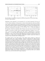
Fig. 1. The respective membership functions for CR (credit line), age, CB (current balance)
and payment.


Hence, μ
An
, μ
Bn
, μ
Cn
and μ
Dn
denote fuzzy membership functions for a credit line, age,
current balance and payment, respectively. n is the center of a triangular fuzzy set. The
triangular fuzzy sets are plotted in Fig. 1. L, M, H, and VH denote the linguistic variables
low, medium, high, very high in the amount feature. Y, M and O denote the linguistic

variables young, middle and old for the age feature. Next, the fuzzy rules are created. The
rule sets are shown in Tables 10 and 11.
Then, weights are assigned to each linguistic term using subsethood values. Next,
the fuzzy membership values are calculated for each linguistic term in each subgroup as
given in Tables 10 and 11. The fuzzy membership values are calculated according to each
New Developments in Robotics, Automation and Control

240
classification result. Finally, the classification is calculated using the de-fuzzification to get a
single value that represents the output fuzzy set, namely the risk ratio.

Current balance
Payment
Very high High Medium Low
Very high Common Good Excellent Excellent
High Good Common Good Excellent
Medium Worst Worst Common Good
Low Worst Worst Worst Common
Table 10. Current balance to payment linguistic labels matrix.

Credit line
Age
Very high High Medium Low
Young Good Common Common Worst
Middle Excellent Good Common Common
Old Common Common Worst Worst
Table 11. Credit line to age linguistic labels matrix.

4.4 Input output coding
Three types of input variables are used, namely qualitative, quantitative (or numeric) and

ratio (Durham University, 2008). A binary encoding scheme is used to represent the
presence 1, or absence 0, of a particular (qualitative) data. Quantitative data are normalized
into the range [0, 1]. Ratios are the proportion of related variables calculated to signal the
importance of data. We encode ratios by computing the proportion of related variables to
describe the importance of the data.
Input variables comprise (1) gender, encoded using one bit (0 = female, 1 = male),
(2) customer age, denotes the customer age between 20 and 80 years, (3) age of the client
account, from 1 to 13 years, (4) current balance, denotes the total amount of money owed by
cardholders in the range from 1 to 1,000,000, (5) payment amount, denotes the total amount of
money debited by cardholders and is in the range from 1 to 1,000,000, (6) transaction amount,
denotes the total amount of money consumed by cardholders from 1 to 1,000,000, (7)
delinquent flag, records the status that late payments have been received and is encoded into
3 binary bits, where 000 indicates full pay, 001 minimum monthly payment, 010 delinquent
within one month, 011 delinquent within two to four months, 100 delinquent within five to
seven months and 101 delinquent above seven months, (8) risk ratio, is given by the FMS and
encoded into one ratio bit, (9) payment amount to current balance ratio, denotes solvency and is
encoded into one ratio bit.
The two output variables signal the cardholder status. These are coded as 00 normal,
01 bad debt or 10 charge-off accounts.

5. Experimental Results

The tools used for implementing the experimental system include JBUILDER 9.0, SQL 2000
and Windows 2000. Input values were normalized to the range from 0 to 1. After training,
Intelligent Detection of Bad Credit Card Accounts

241
the neural network is capable of classifying credit status. A predefined threshold of 0.8 was
used to detect suspicious cases.

5.1 Procedure
A small dataset, provided by a local bank in Taiwan, was used to demonstrate how this
method works. This data set contains 449,256 accounts belonging to three classes; namely
433,961 normal accounts, 10,105 bad debt accounts, and 5,190 charge-off accounts. There are
only 0.35% abnormal accounts in practice. The experimental data set is divided into two
subsets, namely 3,000 training examples and 10,000 test examples. The training set
comprises 1,000 normal accounts, 1,000 bad accounts and 1,000 charge-off accounts. A two-
way cross validation table was used to select input features. To obtain good input features a
fuzzy rule-based system was incorporated. A risk ratio of variables with fuzzy value was
created to enhance the prediction accuracy. After data transformation, the features to be
input to the BPN were encoded in the [0, 1] interval. The BPN classifies input into one of
three classes. The network is repetitively trained with different network parameters until it
converges. We randomly selected 3,000 training examples from the total sample, where
1,000 examples were normal accounts, 1,000 were bad dept account and 1,000 were charge-
off accounts.
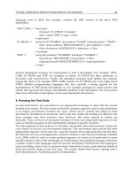
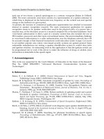
The neural network learning parameters need to be set to avoid the effect of over-
fitting and to maintain reasonable performance. Fig. 2 and 3 show system screenshots of the
two main views. The learning parameters were tuned by running the simulations multiple
times.
The back-propagation network comprised 11 input nodes, 7 hidden nodes, and 2
output nodes. The coding of the output vectors were as follows: bad debt accounts (1,0),
charge-off accounts (0,1) and normal accounts (0,0). Table 12 shows BPN typical input
output mapping examples.


Fig. 2. The training screen.
New Developments in Robotics, Automation and Control

242

Fig. 3. The test screen.

Name Type I/O bad debt charge-off normal
X1 Binary Input 1 1 0
X2 Quantification Input 0.25 0.31 0.51
X3 Quantification Input 0.18 0.23 0.23
X4 Quantification Input 0.45 0.95 0.17
X5 Quantification Input 0.18 0.15 0.36
X6 Quantification Input 0.15 0.15 0.16
X7 Binary Input 010 101 000
X8 Ratio Input 0.44 0.95 0.16
X9 Ratio Input 0.29 0.15 0.15
O1 Binary Output 0.9997 0.0091 0.0215
O2 Binary Output 0.0002 0.9905 0.0286
Table 12. Neural network mapping examples.
Intelligent Detection of Bad Credit Card Accounts

243
5.2 Performance Evaluation
Performance was measured in terms of precision and recall. Precision is defined as the
proportion of classified instances that were correctly classified, and recall as the proportion
of instances classified correctly (Cohn, 2003), or formally


,
)(
)()(
qR
qRqA
recall

∩
=
(16)

.
)(
)()(
qA
qRqA
precision
∩
=
(17)

5.3 Detection Performance
We started with a network with all possible input nodes. But all possible nodes are never
needed to represent a system. Therefore, we used two-way cross validations to filter off
redundant input features. Besides, we designed risk ratio of variables to raise the
performance. We fixed the network parameters and set the initial learning rate to 10 with a
decreasing rate of 0.001. We consolidated the performance achieved with the fuzzy BPN and
the non-fuzzy BPN (see Table 13). Clearly, the fuzzy BPN yields better results than the
conventional BPN.

Proposed detection model Conventional BPN model
Iterations
Recall (R1) Precision (P1) Recall (R2) Precision (P2)
100 85.20% 79.00% 75.80% 65.00%
200 87.95% 84.00% 80.15% 72.00%
300 88.30% 83.90% 81.30% 73.00%
500 90.00% 85.00% 83.60% 76.80%

1000 95.50% 95.00% 86.00% 80.00%
2000 95.35% 94.97% 86.15% 80.20%
Average 90.38% 86.98% 82.17% 74.50%
Table 13. The performance of the proposed detection model versus conventional BPN
detection.

Additionally, a dataset comprising 10,000 simulated entries were used to evaluate and
validate the system, where different normal to abnormal data ratios were considered to
diagnose different behaviours. The results are listed in Table 14, and each experiment shows
the size of the detected set, the number of addressed problems, the total precision P and the
New Developments in Robotics, Automation and Control

244
total recall R rates. This experimental evidence demonstrates that the strategy is capable of
effectively tackling more than 90% of the problems.

Number of addressed problems
Result
Size
Normal Bad debt Charge-off
Recall Precision
Test Data-1 282 9706 137 145 94.00% 95.59%
Test Data-2 4512 5177 2036 2476 90.24% 93.55%
Test Data-3 5372 4068 2420 2952 89.53% 90.56%
Table 14. The comparisons of test results from different iterations.

5.4 Implications
The strategy outlined herein could be used for risk management, analysis of business rules,
delinquent diagnosis and abnormal accounts forecasting. Risk management helps reduce
issuers’ losses due to bad debt. When detecting bad debt accounts, the issuers can reduce the

credit line. Moreover cardholders can be offered realistic loan plans to help them overcome
their financial difficulties (Lin, 2003). Analysis of business rules is used to establish a way to
normalize the analysis that facilitates to compare the business rules across various types of
credit card accounts. We could take these rules to develop a business model in the
knowledge management system. Delinquent diagnosis is used to analyze the existing
delinquent factors as a high-level understanding of process and control systems of an
application. Delinquent diagnosis is a way to monitor the delinquent accounts early to avoid
losses due to bad debt. Abnormal account forecasting is commonly used to recognize
portfolio dynamics and behaviour patterns.

6. Conclusions and Future Work

A novel scheme for the bad credit account detection was proposed. A fuzzy rule-based
system was used to provide inputs for a back-propagation neural network that was used for
classifying accounts. The proposed system has been tested on real credit data and it is
capable of detecting bad accounts in the large data set with a success rate of more than 90%.
Future work includes integrating the proposed system with credit card risk management
systems and the introduction of noise reduction mechanism for discarding outlier accounts,
i.e., observations that deviates so much from other observations as to arouse suspicion that
it was generated by a different mechanism. Finally, it would be desirable to integrate other
AI algorithms (e.g., GA) with data mining to enhance predictive accuracy and apply the
algorithm to relational (e.g., spatial) data.

7. References

Aleskerov, E.; Freisleben, B. & Rao, B. (1997). CARDWATCH: a neural network based
database mining system for credit card fraud detection. Proceedings of IEEE Int.
Conf. on Computational Intelligence for Financial Engineering, pp. 220-226, NY, USA,
March 1997.
Intelligent Detection of Bad Credit Card Accounts

245
Brause, R.; Langsdorf, T. & Hepp, M. (1999). Neural data mining for credit card fraud
detection. Proceedings of 11th IEEE Int. Conf. on Tools with Artificial Intelligence, pp.
103-106, Chicago, IL, USA, November 1999.
Burns, P. & Stanley, A. (2001). Managing consumer credit risk. Federal Reserve Bank of
Philadelphia Payment Cards Center Discussion Paper, no. 01-03, pp. 1-7, November
2001.
Chakraborty, D. & Pal, N.R. (2001). Integrated feature analysis and fuzzy rule-base system
identification in a neuro-fuzzy paradigm. IEEE Trans. Systems, Man, and Cybernetics,
vol. 31, no. 4, pp. 391-400, June 2001.
Chiang, S.C. (2003). The relationship between credit-evaluation factors and credit card default risk—
an example of the credit cards issued by the a financial institute in Taiwan. Master Thesis,
Department of Insurance, Feng Chia University, Taichung, Taiwan, June 2003.
Cohn, T. (2003). Performance metrics for word sense disambiguation. Proceedings of the
Australasian Language Technology Workshop, pp. 49-56, Victoria, Australia, December
2003.
Huang, Y P.; Chang, T W.; Chen, Y R. & Sandnes, F.E. (2008). A back propagation based
real-time license plate recognition system. Int. Journal of Pattern Recognition and
Artificial Intelligence, vol. 22, no. 2, pp. 233-251, March 2008.
Huang, Y P. & Hsieh, W J. (2003). The application of grey model and back-propagation
network to establish the alarm mechanism for the premium rate service. Journal of
Grey System, vol. 6, no. 2, pp. 75-88, December 2003.
Huang, Y P.; Hsu, L W. & Sandnes, F.E. (2007). An intelligent subtitle detection model for
locating television commercials. IEEE Trans. on Systems, Man, and Cybernetics, Part
B: Cybernetics, vol. 37, no. 2, pp. 485-492, April 2007.
Huang, Y P.; Huang, Y H. & Sandnes, F.E. (2006). A fuzzy inference model-based non-
reassuring fetal status monitoring system. Int. Journal of Fuzzy Systems, vol. 8, no.
1, pp. 57-64, March 2006.
Kijsirikul, B. & Chongkasemwongse, K. (2001). Decision tree pruning using backpropagation

neural networks. Proceedings of IEEE Int. Conf. on Neural Networks, vol. 3, pp. 1876-
1880, Washington D.C., USA, Month 2001.
Kuo, Y.F.; Lu, C.T.; Sirwongwattana, S. & Huang, Y P. (2004). Survey of fraud detection
techniques. Proceedings of IEEE Int. Conf. on Networking, Sensing and Control, pp. 749-
754, Taipei, Taiwan, March 2004.
Lee, H.M.; Chen, C.M.; Chen, J.M. & Jou, Y.L. (2001). An efficient fuzzy classifier with
feature selection based on fuzzy entropy. IEEE Trans. on Systems, Man and
Cybernetics, vol. 31, no. 3, pp.426-432, June 2001.
Lee, M.H. (2002). A study on the credit risk of the credit card holder. Master Thesis, Department
of Insurance, Feng Chia University, Taichung, Taiwan, June 2001.
Lin, C.J. (2003). Data mining for risk improving of credit card. Master Thesis, Department of
Computer Science and Engineering, Tamkang University, Taipei, Taiwan, June
2003.
Lin, J. (2005). Interest-rate cap dropped as bankers offer relief plan. Taipei Times, Friday, Dec.
16, 2005.
Yu, H.H. (2003). The research of applying improved artificial neural network to credit card customer
relationship management. Master Thesis, Department of Business Management,
National Taipei University of Technology, Taipei, Taiwan, June 2003.
New Developments in Robotics, Automation and Control

246
Zhang, D. & Zhou, L. (2004). Discovering golden nuggets: data mining in financial
application. IEEE Trans. on Systems, Man, and Cybernetics—Part C: Applications and
Reviews, vol. 34, no. 4, pp. 513-522, November 2004.
Cardservice International website (2008), .
Central Bank of China website (2008), .
Durham University website (2008), .
Indiana University Office of the Treasurer website (2008), .
National Credit Card Center of R.O.C website (2008), .
ShopSite website (2008), .

Taiwan Financial Supervisory Commission website (2008), .
Taiwan Joint Credit Information Center website (2008), .
The International Commercial Bank of China website (2008), .

14

Improved Chaotic Associative Memory
for Successive Learning

Takahiro IKEYA and Yuko OSANA
Tokyo University of Technology
Japan

1. Introduction

Recently, neural networks are drawing much attention as a method to realize flexible
information processing. Neural networks consider neuron groups of the brain in the
creature, and imitate these neurons technologically. Neural networks have some features,
especially one of the important features is that the networks can learn to acquire the ability
of information processing.
In the filed of neural network, many models have been proposed such as the Back
Propagation algorithm (Rumelhart et al., 1986), the Self-Organizing Map (Kohonen, 1994),
the Hopfield network (Hopfield, 1982) and the Bidirectional Associative Memory (Kosko,
1988). In these models, the learning process and the recall process are divided, and therefore
they need all information to learn in advance.
However, in the real world, it is very difficult to get all information to learn in advance. So
we need the model whose learning and recall processes are not divided. As such model,
Grossberg and Carpenter proposed the Adaptive Resonance Theory (ART) (Carpenter &
Grossberg, 1995). However, the ART is based on the local representation, and therefore it is
not robust for damage. While in the field of associative memories, some models have been

proposed (Watanabe et al., 1995; Osana & Hagiwara, 1999; Kawasaki et al., 2000; Ideguchi et
al., 2005). Since these models are based on the distributed representation, they have the
robustness for damaged neurons. However, their storage capacity is very small because
their learning processes are based on the Hebbian learning. In contrast, the Hetero Chaotic
Associative Memory for Successive Learning with give up function (HCAMSL) (Arai &
Osana, 2006) and the Hetero Chaotic Associative Memory for Successive Learning with
Multi-Winners competition (HCAMSL-MW) (Ando et al., 2006) have been proposed in
order to improve the storage capacity.
In this research, we propose an Improved Chaotic Associative Memory for Successive
Learning (ICAMSL). The proposed model is based on the Hetero Chaotic Associative
Memory for Successive Learning with give up function (HCAMSL) (Arai & Osana, 2006)
and the Hetero Chaotic Associative Memory for Successive Learning with Multi-Winners
competition (HCAMSL-MW) (Ando et al., 2006). In the proposed ICAMSL, the learning
process and recall process are not divided. When an unstored pattern is given to the
New Developments in Robotics, Automation and Control

248
network, the ICAMSL can learn the pattern successively. Moreover, the storage capacity of
the proposed ICAMSL is larger than that of the conventional HCAMSL/HCAMSL-MW.

2. Chaotic Neural Network

A neural network composed of the chaotic neurons is called a chaotic neural network
(Aihara et al., 1990).
The dynamics of the chaotic neuron
i in the neural network composed of N chaotic
neurons is represented by the following equation:

() () () ()
∑∑ ∑∑∑

== ===
⎥
⎥
⎦
⎤
−−−−+
⎢
⎢
⎣
⎡
−=+
N
j
t
d
t
d
ii
d
rj
d
mij
t
d
j
d
s
M
j
iji

dtxkdtxkwdtAkvftx
10 001
1
θα
(1)

where
)(tx
i
shows the output of the neuron i at the time t ,
M
is the number of the
external inputs,
ij
v is the connection weight from the external input
j
to the neuron i ,
)(tA
j
is the strength of the external input
j
at the time t ,
ij
w is the connection weight
between the neuron
i and the neuron
j
,
α
is the scaling factor of the refractoriness,

s
k
,
m
k
and
r
k
are the damping factors and
i
θ
is the threshold of the neuron i .
()
⋅f is the
following output function:

()
()
ε
/exp1
1
u
uf
−+
=
(2)
where
ε
is the steepness parameter. It is known that dynamic associations can be realized
in the associative memories composed chaotic neurons.

3. Multi Winners Self-Organizing Neural Network

Here, we briefly explain the Multi Winners Self-Organizing Neural Network (MWSONN)
(Huang & Hagiwara., 1997) which is used in the proposed model.
Figure 1 shows the structure of the MWSONN. The MWSONN consists of the Input/Output
Layer and the Distributed Representation Layer, and each layer has 2- dimensional structure.
In the learning process of the MWSONN, the distributed representation patterns
corresponding to input analog patterns are generated by the multi winners self-organizing
process, and the connection weights between layers are trained by the error correction
learning. In the recall process of the MWSONN, when a stored pattern or a part of the stored
patterns is given to the Input/Output Layer, the corresponding distributed representation
pattern appears in the Distributed Representation Layer, and then the corresponding analog
pattern appears in the Input/Output Layer.
Improved Chaotic Associative Memory for Successive Learning

249

Fig. 1. Structure of MWSONN.

4. Improved Chaotic Associative Memory for Successive Learning

4.1 Outline of ICAMSL
Here, we explain the outline of the proposed Improved Chaotic Associative Memory for
Successive Learning (ICAMSL). The proposed ICAMSL has three stages; (1) Pattern Search
Stage, (2) Distributed Pattern Generation Stage and (3) Learning Stage.
When an unstored pattern set is given to the network, the proposed ICAMSL distinguishes
an unstored pattern set from stored patterns and can learn the pattern set successively.
When a stored pattern set is given, the ICAMSL recalls the patterns. When an unstored
pattern set is given to the network, the ICAMSL changes the internal pattern for input

pattern set by chaos and presents other pattern candidates (we call this the Pattern Search
Stage). When the ICAMSL can not recall the desired patterns, the distributed pattern is
generated by the multi-winners competition (Huang & Hagiwara., 1997) (Distributed
Pattern Generation Stage), and it learns the input pattern set as an unstored pattern set
(Learning Stage). Figure 2 shows the flow of the proposed ICAMSL.

4.2 Structure of ICAMSL
The proposed ICAMSL is a kind of the hetero-associative memories. Figure 3 shows a
structure of the ICAMSL. This model has two layers; an Input/Output Layer (I/O Layer)
composed of conventional neurons and a Distributed Representation Layer (DR Layer)
composed of chaotic neurons (Aihara et al., 1990). In this model, there are the connection
weights between neurons in the Distribute Representation Layer and the connection weights
between the Input/Output Layer and the Distributed Representation Layer.
As shown in Fig.3, the Input/Output Layer has plural parts. The number of parts is decided
depending on the number of patterns included in the pattern set. In the case of Fig.3, the
Input/Output Layer consists of P parts corresponding to the patterns P
~
1 .
In this model, when a pattern set is given to the Input/Output Layer, the internal pattern
corresponding to the input patterns is formed in the Distributed Representation Layer. Then,
New Developments in Robotics, Automation and Control

250

Fig. 2. Flow of Proposed ICAMSL.

in the Input/Output Layer, an output pattern set is generated from the internal pattern. The
ICAMSL distinguishes an unstored pattern set from stored patterns by comparing the input
patterns with the output pattern.
In this model, the output of the neuron

i
in the Distributed Representation Layer at the time
1+
t ,
()
1+tx
i
is given by the following equations.


(
)
(
)
(
)
(
)
[
]
1111
+
+
+
+
+
=
+
ttttx
iiii

ζ
η
ξ
φ
(3)
() ( )
() ()
∑
∑∑
=
==
+=
−=+
M
j
jijis
t
d
j
d
s
M
j
iji
tAvtk
dtAkvt
1
01
1
ξ

ξ
(4)
() ( )
() ()
∑
∑∑
=
==
+=
−=+
N
j
jijim
t
d
j
d
m
N
j
iji
txwtk
dtxkwt
1
01
1
η
η
(5)
Improved Chaotic Associative Memory for Successive Learning

251
() ( )
() () ( )
riiir
t
d
ii
d
ri
ktxtk
dtxkt
−−−=
−−−=+
∑
=
1
1
0
θαζ
θαζ
(6)

In Eqs.
() ()
6~3
,
M
is the number of neurons in the Input/Output Layer,
ij

v is the
connection weight between the neuron
j
in the Input/Output Layer and the neuron i in
the Distributed Representation Layer,
N is the number of neurons in the Distributed
Representation Layer,
(
)
tA
j
is the external input
j
to the Input/Output Layer at the time
t
,
ij
w is the connection weight between the neuron i and the neuron
j
in the Distributed
Representation Layer,
(
)
t
α
is the scaling factor of the refractoriness at the time
t
, and
s
k ,

m
k and
r
k are the damping factors.
(
)
⋅
φ
is the following output function:

(
)
(
)
ε
φ
/tanh
ii
uu
=
(7)
where
ε
is the steepness parameter.
The output of the neuron
j
in the Input/Output Layer at the time
t
,
(

)
tx
IO
j
is given as
follows.

() ()
⎟
⎟
⎠
⎞
⎜
⎜
⎝
⎛
=
∑
=
N
i
D
iij
IOIO
j
txvtx
1
φ
(8)
⎩

⎨
⎧
<−
≥
=
0,1
0,1
u
u
IO
φ
(9)

4.3 Pattern Search Stage
In the Pattern Search Stage, when an input pattern set is given, the ICAMSL distinguishes
the pattern set from stored patterns. When an unstored pattern set is given, the ICAMSL
changes the internal pattern for the input pattern by chaos and presents the other pattern
candidates. Until the ICAMSL recalls the desired patterns, the following procedures are
repeated. If the ICAMSL can not recall the desired patterns, when the stage is repeated
certain times, the ICAMSL finishes the stage.

4.3.1 Pattern Assumption
In the proposed ICAMSL, only when the input patterns are given to all parts of the
Input/Output Layer, the patterns are judged. When the input pattern
(
)
tA is similar to the
recalled pattern
(
)

tx
IO
, the ICAMSL can assume that input pattern is one of the stored
patterns. The ICAMSL outputs the pattern formed by the internal pattern in the Distributed
Representation Layer. The similarity
(
)
ts is defined by

() () ()
.
1
1
∑
=
=
M
j
IO
jj
txtA
M
ts
(10)
New Developments in Robotics, Automation and Control

252
The ICAMSL regards the input patterns as a stored pattern set, when the similarity rate
()
ts

is larger than the threshold
(
)
(
)
thth
stss ≥ .


Fig. 3. Structure of Proposed ICAMSL.

4.3.2 Pattern Search
When the ICAMSL assumes that the input patterns are an unstored pattern set, the ICAMSL
changes the internal pattern
(
)
tx
D
for the input pattern by chaos and presents the other
pattern candidates.
In the chaotic neural network, it is known that dynamic association can be realized if the
scaling factor of the refractoriness
(
)
t
α
is suitable (Aihara et al., 1990). Therefore, in the
proposed model,
(

)
t
α
is changed as follows:

(
)
(
)
(
)
(
)
(
)
(
)
DIV
tstt
α
α
α
α
α
/1
minminmax
+
−
−
=

(11)

(
)
maxmaxmax
NwMvt
+
=
α
(12)

{
}
NMij
vvvv ,,,, max
11max
LL= (13)

{
}
NNii
wwww ,,,, max
11max
LL
′
= (14)

where
min
α

is the minimum of
α
,
(
)
t
max
α
is the maximum of
α
at the time t ,
()
ts is the
similarity between the input pattern and the output pattern at the time
t (the time when the
Pattern Search Stage started), and
DIV
α
is the constant.
4.4 Distributed Pattern Generation Stage
In the Distributed Pattern Generation Stage, the distributed pattern corresponding to the
input pattern is generated by the multi-winners competition (Huang & Hagiwara., 1997).
Improved Chaotic Associative Memory for Successive Learning

253
4.4.1 Calculation of Outputs of Neurons in I/O Layer
When the input pattern
(
)
tA

j
is given to the Input/Output Layer, the output of the neuron
j
in the Input/Output Layer
IO
j
x is given by
(
)
(
)
tASx
jf
IO
j
=
(15)
where
()
⋅
f
S is the ramp function and is given by

()
⎩
⎨
⎧
≤
>
=

.0,0
0,
u
uu
uS
f
(16)

4.4.2 Calculation of Initial Outputs of Neurons in DR Layer
The output of the neuron
i
in the Distributed Representation Layer
(
)
0D
i
x is calculated by

()
⎟
⎟
⎠
⎞
⎜
⎜
⎝
⎛
−=
∑
=

M
j
i
IO
jijf
D
i
xvCx
1
0
θ
(17)
where
ij
v is the connection weight from the neuron
j
in the Input/Output Layer to the
neuron
i in the Distributed Representation Layer,
i
θ
is the threshold of the neuron i in the
Distributed Representation Layer and
M
is the number of neurons in the Input/Output
Layer. The output function
(
)
⋅
f

C is given by

(
)
(
)
TuuC
f
/tanh=
(18)
where
T
is the steepness parameter in the sigmoidal function.

4.4.3 Competition between Neurons in DR Layer
The competition dynamics is given by the following equations:

(
)
iif
D
i
uCx
θ
−=
(19)
∑
=
′
′′

=
N
i
D
iiii
xwu
1
(20)

where
D
i
x
is the output of the neuron i in the Distributed Representation Layer,
i
u is the
internal state of the neuron
i in the Distributed Representation Layer and N is the number
of neurons in the Distributed Representation Layer.

4.5 Learning Stage
In the Pattern Search Stage, if the ICAMSL can not recall the desired pattern set, it learns the
input pattern set as an unstored pattern set. The Learning Stage has two phases; (1) Hebbian
New Developments in Robotics, Automation and Control

254
Learning Phase and (2) anti-Hebbian Learning Phase. If the signs of the outputs of two
neurons are same, the connection weight between these two neurons is strengthened. By
this learning, the connection weights are changed to learn the input patterns, however the
Hebbian learning can only learn a new input pattern set. In the proposed ICAMSL, the anti-

Hebbian Learning Phase is employed as similar as the original HCAMSL (Arai & Osana,
2006). In the anti-Hebbian Learning Phase, the connection weights are changed in the
opposite direction in the case of the Hebbian Learning Phase. The proposed ICAMSL can
learn a new pattern set without destroying the stored patterns by the anti-Hebbian Learning.
Figure 4 shows the learning stage of the proposed ICAMSL.

4.5.1 Hebbian Learning Phase
In the Hebbian Learning Phase, until the similarity rate
(
)
ts
becomes 1.0, the update of the
connection weights is repeated.
The connection weight between the Input/Output Layer and the Distributed Representation
Layer
ij
v and the connection weight in the Distributed Representation Layer
ii
w
′
are
updated as follows:


(
)
(
)
(
)

(
)
tAxvv
j
compD
iv
old
ij
new
ij
+
+=
γ
(21)

(
)
(
)
(
)
(
)
compD
i
compD
iw
old
ii
new

ii
xxww
′
+
′′
+=
γ
(22)
where
+
v
γ
is the learning rate of the connection weight
ij
v in the Hebbian Learning Phase,
and
+
w
γ
is the learning rate of the connection weight
ii
w
′
in this phase.

4.5.2 Give Up Function
When the similarity rate
(
)
ts does not become 1.0 even if the connection weights are

updated
n
T times, the ICAMSL gives up to memorize the pattern set. If the ICAMSL gives
up to learn the pattern set, the anti-Hebbian Learning Phase is not performed.

4.5.3 Anti-Hebbian Learning Phase
The anti-Hebbian Learning Phase is performed after the Hebbian Learning Phase. In this
phase, the connection weight
ij
v and
ii
w
′
are changed in the opposite direction in the case
of the Hebbian Learning Phase. The anti-Hebbian Learning makes the relation between the
patterns is learned without destroying the stored patterns.
In this phase,
ij
v and
ii
w
′
are updated by

(
)
(
)
(
)

(
)
tAxvv
j
compD
iv
old
ij
new
ij
−
+=
γ
(23)

(
)
(
)
(
)
(
)
compD
i
compD
iw
old
ii
new

ii
xxww
′
−
′′
+=
γ
(24)
Improved Chaotic Associative Memory for Successive Learning

255
where
(
)
0>>
+−−
vvv
γγγ
is the learning rate of the connection weight
ij
v in the anti-Hebbian
Learning Phase, and
(
)
0>>
+−−
www
γγγ
is the learning rate of the connection weight
ii

w
′
in this
phase.


Fig. 4. Learning Stage.

5. Computer Experiment Results

In this section, we show the computer experiment results to demonstrate the effectiveness of
the proposed ICAMSL. The computer experiments were carried out under the conditions
shown in Table 1.



5.1 Successive Learning and One-to-Many Associations
Figure 5 shows the successive learning and one-to-many associations in the proposed
ICAMSL. As seen in Fig.5, the patterns “lion”, “mouse” and “penguin” were given to the
network at
1=t . At 1
=
t , the ICAMSL could not recall the correct patterns because no
pattern was stored in the network. During
11~2
=
t , the ICAMSL changed the internal
patterns by chaos and presented the other pattern candidates, however it could not recall the
correct patterns. As a result, the ICAMSL regarded the input patterns as unstored patterns,
at 13=t , the patterns “lion”, “mouse” and ”penguin” were trained as new patterns. At

14=t , the patterns “lion”, “mouse” and “duck” were given to the network. At this time,
since only the pattern set “lion”, “mouse” and “penguin” was memorized in the network,
the ICAMSL recalled the patterns “lion”, ”mouse” and “penguin”. During
24~15=t , the
ICAMSL changed the internal patterns by chaos and presented the other pattern candidates,
however it could not recall the correct patterns. As a result, the ICAMSL regarded the input
patterns as unstored patterns, at 28
=
t , the “lion”, ”mouse” and “duck” were trained as
new patterns. At
29
=
t , the patterns “lion” and “mouse” were given to the network, the
ICAMSL recalled “lion”, ”mouse” and “penguin”
(
)
30
=
t and “lion”, “mouse” and
“duck”
()
35=t
. From these results, we confirmed that the proposed ICAMSL can learn
patterns successively and realize one-to-many associations.
New Developments in Robotics, Automation and Control

256
Learning Parameters
the number of pattern searches in Pattern Search Stage 10
initial value of all connection weights 0.1~0.1

−

learning rate in Hebbian Learning
++
wv
γγ
, 1.0
learning rate in anti-Hebbian Learning
−−
wv
γγ
, 2.0
threshold of similarity rate
th
s 1.0
Chaotic Neuron Parameters
constant for refractoriness
DIV
α
25
minimum of scaling facter
α

min
α
0.0
damping factor
s
k 0.5
damping factor

m
k 0.0
damping factor
r
k 0.95
threshold of neurons
θ
0.0
steepness parameter
ε
1.0
Competition Parameters
steepness parameter
T
0.0005
Table 1. Experimental Conditions.

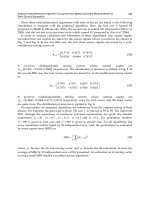
5.2 Storage Capacity
Here, we examined the storage capacity of the proposed ICAMSL. In this experiment, we
used the ICAMSL which has 800 neurons (400 neurons for pattern 1 and 400 neurons for
pattern 2) in the Input/Output Layer and 225 neurons in the Distributed Representation
Layer. We used random patterns to store and Fig.6 shows the average of 100 trials. In this
figure, the horizontal axis is the number of stored pattern pairs, and the vertical axis is the
perfect recall rate. In this figure, the storage capacities of the model without give up function
(HCAMSL-MW) (Ando et al., 2006), the model without the Distributed Pattern Generation
Stage (HCAMSL) (Arai & Osana, 2006) and the model without the give up function and the
Distributed Pattern Generation Stage are also shown for reference.
From these results, we confirmed that the storage capacity of the proposed ICAMSL is
larger than that of the conventional HCAMSL/HCAMSL-MW.

6. Conclusions

In this research, we have proposed the Improved Chaotic Associative Memory for
Successive Learning (ICAMSL). The proposed model is based on the Hetero Chaotic
Associative Memory for Successive Learning with give up function (HCAMSL) (Arai &
Osana, 2006) and the Hetero Chaotic Associative Memory for Successive Learning with
Multi-Winners competition (HCAMSL-MW)
(Ando et al., 2006). In the proposed ICAMSL,
the learning process and recall process are not divided. When an unstored pattern is given
to the network, the ICAMSL can learn the pattern successively. We carried out a series of
computer experiments and confirmed that the proposed ICAMSL can learn patterns
Improved Chaotic Associative Memory for Successive Learning

257
successively and realize one-to-many associations, and the storage capacity of the ICAMSL
is larger than that of the conventional HCAMSL/HCAMSL-MW.


(a) t=1 (b) t=2 (c) t=11

(d) t=13 (e) t=14 (f) t=15

(g) t=24 (h) t=28 (i) t=29


(j) t=30 (k) t=35
Fig. 5. Successive Learning in Proposed Model.


Fig. 6. Storage Capacity.