High Performance Computing in Remote Sensing - Chapter 17 docx

Chapter 17
Real-Time Online Processing of
Hyperspectral Imagery for Target Detection
and Discrimination
Qian Du,
Missisipi State University
Contents
17.1 Introduction 398
17.2 Real-Time Implementation 399
17.2.1 BIP Format 399
17.2.2 BIL Format 401
17.2.3 BSQ Format 401
17.3 Computer Simulation 402
17.4 Practical Considerations 404
17.4.1 Algorithm Simplification Using R
−1
404
17.4.2 Algorithm Implementation with Matrix Inversion 405
17.4.3 Unsupervised Processing 405
17.5 Application to Other Techniques 407
17.6 Summary 407
Acknowledgment 408
References 408
Hyperspectral imaging is a new technology in remote sensing. It acquires hundreds
of images in very narrow spectral bands (normally 10nm wide) for the same area
on the Earth. Because of higher spectral resolutions and the resultant contiguous
spectral signatures, hyperspectral image data are capable of providing more accurate
identification ofsurfacematerials than multispectral data,and areparticularly usefulin
national defense related applications. The major challenge of hyperspectral imaging
is how to take full advantage of the plenty spectral information while efficiently
handling the data with vast volume.

In some cases, such as national disaster assessment, law enforcement activities, and
military applications, real-time data processing is inevitable to quickly process data
and provide the information for immediate response. In this chapter, we present a real-
time online processing technique using hyperspectral imagery forthe purpose oftarget
397
© 2008 by Taylor & Francis Group, LLC
398 High-Performance Computing in Remote Sensing
detection and discrimination. This technique is developed for our proposed algorithm,
called the constrained linear discriminant analysis (CLDA) approach. However, it is
applicable to quite a few target detection algorithms employing matched filters. The
implementation scheme is also developed for different remote sensing data formats,
such as band interleaved by pixel (BIP), band interleaved by line (BIL), and band
sequential (BSQ).
17.1 Introduction
We have developed the constrained linear discriminant analysis (CLDA) algorithm
for hyperspectral image classification [1, 2]. In CLDA, the original high-dimensional
data are projectedonto a low-dimensional space as done by Fisher’s LDA, but different
classes are forced to be along different directions in this low-dimensional space. Thus
all classes are expected to be better separated and the classification is achieved simul-
taneously with the CLDA transform. The transformation matrix in CLDA maximizes
the ratio of interclass distance to intraclass distance while satisfying the constraint
that the means of different classes are aligned with different directions, which can be
constructed by using an orthogonal subspace projection (OSP) method [3] coupled
with a data whitening process. The experimental results in [1],[2] demonstrated that
the CLDA algorithm could provide more accurate classification results than other
popular methods in hyperspectral image processing, such as the OSP classifier [3]
and the constrained energy minimization (CEM) operator [4]. It is particularly useful
to detect and discriminate small man-made targets with similar spectral signatures.
Assume that there are c classes and the k-th class contains N
k

patterns. Let N =
N
1
+ N
2
+···N
c
be the number of pixels. The j-th pattern in the k-th class, denoted
by x
k
j
= [x
k
1 j
, x
k
2 j
, ···, x
k
Lj
]
T
,isanL-dimensional pixel vector (L is the number
of spectral bands, i.e., data dimensionality). Let μ
k
=
1
N
k


N
k
j=1
x
k
j
be the mean of
the k-th class. Define J (F) to be the ratio of the interclass distance to the intraclass
distance after a linear transformation F, which is given by
J(F) =
2
c(c−1)

c−1
i=1

c
j=i+1
F(μ
i
) − F(μ
j
)
2
1
CN

c
k=1
[


N
k
j=1
F(x
N
k
j
) − F(μ
k
)
2
]
(17.1)
and
F(x) = (W
L×c
)
T
; x = [w
1
, w
2
, ···, w
c
]
T
x (17.2)
The optimal linear transformation F
∗

is the one that maximizes J(F) subject to
t
k
= F(μ
k
) for all k, where t
k
= (0 ···01 ···0)
T
is a c × 1 unit column vector with
one in the k-th component and zeros elsewhere. F
∗
can be determined by
w
∗
i
= ˆμ
i
T
P
⊥
ˆ
U
i
(17.3)
© 2008 by Taylor & Francis Group, LLC
Real-Time Online Processing of Hyperspectral Imagery for Target Detection 399
where
P
⊥

ˆ
U
i
= I −
ˆ
U
i
(
ˆ
U
T
i
ˆ
U
i
)
−1
ˆ
U
T
i
(17.4)
with
ˆ
U
i
= [ˆμ
1
··· ˆμ
j

··· ˆμ
c
]
j=i
and I the identity matrix. The ‘hat’ operator specifies
the whitened data, i.e.,
ˆ
x = P
T
w
x, where P
w
is the data whitening operator.
Let S denote the entire class signature matrix, i.e., c class means. It was proved
in [2] that the CLDA-based classifier using Eqs. (17.4)–(17.5) can be equivalently
expressed as
P
T
k
= [0 ···010 ···0]

S
T

−1
S

−1
S
T


−1
(17.5)
for classifying the k-th class in S, where

is the sample covariance matrix.
17.2 Real-Time Implementation
In our research, we assume that an image is acquired from left to right and from
top to bottom. Three real-time processing fashions will be discussed to fit the three
remote sensing data formats: pixel-by-pixel processing for BIP formats, line-by-line
processing for BIL formats, and band-by-band processing for BSQ formants. In the
pixel-by-pixel fashion, a pixel vector is processed right after it is received and the
analysis result is generated within an acceptable delay; in the line-by-line fashion, a
line of pixel vectors is processed after the entire line is received; in the band-by-band
fashion, a band is processed after it is received.
In order to implement the CLDA algorithm in real time, Eq. (17.6) is used. The
major advantage of using Eq. (17.6) instead of Eqs. (17.4) and (17.5) is the simplicity
of real-time implementation since the data whitening process is avoided. So the key
becomes the adaptation of

−1
, the inverse sample covariance matrix. In other words,

−1
at time t can be quickly calculated by updating the previous

−1
at t −1 using
the data received at time t, without recalculating the


and

−1
completely. As
a result, the intermediate data analysis result (e.g., target detection) is available in
support of decision-making even when the entire data set is not received; and when
the entire data set is received, the final data analysis result is completed (within a
reasonable delay).
17.2.1 BIP Format
This format is easy to handle because a pixel vector of size L ×1 is received contin-
uously. It fits well a spectral-analysis based algorithm, such as CLDA.
© 2008 by Taylor & Francis Group, LLC
400 High-Performance Computing in Remote Sensing
Let the sample correlation matrix R be defined as R =
1
N

N
i=1
x
i
·x
T
i
, which can
be related to

and sample mean μ by

= R − μ · μ

T
(17.6)
Using the data matrix X, Eq. (17.7) can be written as N ·

= X · X
T
− N ·μ ·μ
T
.
If
˜

denotes N ·

,
˜
R denotes N · R, and ˜μ denotes N · ˜μ, then
˜

=
˜
R −
1
N
t
· ˜μ · ˜μ
T
(17.7)
Suppose that at time t we receive the pixel vector x
t

. The data matrix X
t
including
all the pixels received up to time t is X
t
= [x
1
, x
2
, ···, x
t
] with N
t
pixel vectors. The
sample mean, sample correlation, and covariance matrices at time t are denoted as
μ
t
, R
t
, and

t
, respectively. Then Eq. (17.8) becomes
˜

t
=
˜
R
t

−
1
N
t
· ˜μ
t
· ˜μ
T
t
(17.8)
The following Woodbury’s formula can be used to update
˜

−1
t
:
(A + BCD)
−1
= A
−1
− A
−1
B(C
−1
+ DA
−1
B)
−1
DA
−1

(17.9)
where A and C are two positive-definite matrices, and the sizes of matrices A, B, C,
and D allow the operation (A + BCD). It should be noted that Eq. (17.10) is for the
most general case. Actually, A, B, C, and D can be reduced to vector or scalar as long
as Eq. (17.10) is applicable. Comparing Eq. (17.9) with Eq. (17.10), A =
˜
R
t
, B = ˜μ
t
,
C =−
1
N
t
, D = ˜μ
T
t
,
˜

−1
t
can be calculated using the variables at time (t − 1) as
˜

−1
t
=
˜

R
−1
t
+
˜
R
−1
t
˜
u
t
(N
t
−
˜
u
T
t
˜
R
−1
t
˜
u
t
)
−1
˜
u
T

t
˜
R
−1
t
(17.10)
The ˜μ
t
can be updated by
˜μ
t
= ˜μ
t−1
+ x
t
(17.11)
Since
˜
R
t
and
˜
R
t−1
can be related as
˜
R
t
=
˜

R
t−1
+ x
t
· x
T
t
(17.12)
˜
R
−1
t
in Eq. (17.12) can be updated by using the Woodbury’s formula again:
˜
R
−1
t
=
˜
R
−1
t−1
−
˜
R
−1
t−1
x
t
(1 + x

T
t
˜
R
−1
t−1
x
t
)
−1
x
T
t
˜
R
−1
t−1
(17.13)
Note that (1+x
T
t
˜
R
−1
t−1
x
t
) in Eq. (17.14) and (N
t
−

˜
u
T
t
˜
R
−1
t
˜
u
t
) in Eq. (17.11) are scalars.
This means no matrix inversion is involved in each adaptation.
© 2008 by Taylor & Francis Group, LLC
Real-Time Online Processing of Hyperspectral Imagery for Target Detection 401
In summary, the real-time CLDA algorithm includes the following steps:
r
Use Eq. (17.14) to update the inverse sample correlation matrix
˜
R
−1
t
at time t.
r
Use Eq. (17.12) to update the sample mean μ
t+1
at time t +1.
r
Use Eq. (17.11) to update the inverse sample covariance matrix
˜


−1
t+1
at time
t +1.
r
Use Eq. (17.6) to generate the CLDA result.
17.2.2 BIL Format
If the data are in BIL format, we can simply wait for all the pixels in a line to be
received. Let M be the total number of pixels in each line. M pixel vectors can be
constructed by sorting the received data. Assume the data processing is carried out
line-by-line from left to right and top to bottom in an image, the line received at time
t forms a data matrix Y
t
= [x
t1
x
t2
···x
tM
]. Assume that the number of lines received
up to time t is K
t
, then Eq. (17.10) remains almost the same as
˜

−1
t
=
˜

R
−1
t−1
−
˜
R
−1
t−1
˜
u
t
(K
t
M −
˜
u
T
t
˜
R
−1
t
˜
u
t
)
−1
˜
u
T

t
˜
R
−1
t
(17.14)
Eq. (17.11) becomes
˜μ
t
= ˜μ
t−1
+
M

i=1
x
ti
(17.15)
and Eq. (17.12) becomes
˜
R
−1
t
=
˜
R
−1
t−1
−
˜

R
−1
t−1
Y
t
(I
M×M
+ Y
T
t
˜
R
−1
t−1
Y
t
)
−1
Y
T
t
˜
R
−1
t−1
(17.16)
where I
M×M
is an M × M identity matrix. Note that


I
M×M
+ Y
T
t
˜
R
−1
t−1
Y
t

in
Eq. (17.16) is a matrix. This means the matrix inversion is involved in each adaptation.
17.2.3 BSQ Format
If the data format is BSQ, the sample covariance matrix

and its inverse

−1
have
to be updated in a different way, because no single completed pixel vector is available
until all of the data are received.
Let

1
denote the covariance matrix when Band 1 is received, which actually is
a scalar, calculated by the average of pixel squared values in Band 1. Then

1

can
be related to

2
as

2
=


1

12

21

22

, where

22
is the average of pixel squared
values in Band 2,

12
=

21
is the average of the products of corresponding pixel
© 2008 by Taylor & Francis Group, LLC

402 High-Performance Computing in Remote Sensing
values in Band 1 and 2. Therefore,

t
can be related to

t−1
as

t
=


t−1

t−1,t

T
t−1,t

t,t

(17.17)
where

t,t
is the average of pixel squared values in Band t and

t−1,t
= [


1,t
, ···,

j,t
···,

t−1,t
]
T
is a (t −1)×1 vector with

j,t
being the average of the products
of corresponding pixel values in Band j and t. Equation (17.17) shows that the
dimension of

is increased as more bands are received.
When

−1
t−1
is available, it is more cost-effective to calculate

−1
t
by modifying

−1
t−1

with

t,t
and

t−1,t
. The following partitioned matrix inversion formula can
be used for

−1
adaptation.
Let a matrix A be partitioned as A = [
A
11
A
12
A
21
A
22
]. Then its inverse matrix A
−1
can be calculated as


A
11
− A12A
−1
22

A
21

−1
−

A
11
− A12A
−1
22
A
21

−1
A
12
A
−1
22
−

A
22
− A21A
−1
11
A
12


−1
A
21
A
−1
11

A
22
− A21A
−1
22
A
12

−1

(17.18)
Let A
11
=

t−1
, A
22
=

t,t
, A
12

=

t−1,t
, and A
21
=

T
t−1,t
. All these
elements can be generated by simple matrix multiplication. Actually, in this case, no
operation of matrix inversion is used when reaching the final

−1
.
The intermediate result still can be generated by applying the

−1
t
to the first t
bands. This means the spectral features in these t bands are used for target detection
and discrimination. This may help to find targets at early processing stages.
17.3 Computer Simulation
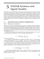
The HYDICE image scene shown in Figure 17.1 was collected in Maryland in 1995
from a flight altitude of 10,000 feet with approximately 1.5m spatial resolution in
0.4–2.5 μm spectral region. The atmospheric water bands with low signal-to-noise
ratio were removed, reducing the data dimensionality from 210 to 169. The image
scene has 128 lines and the number of pixels in each line M is 64, so the total number
of pixel vectors is 128 × 64 = 4096. This scene includes 15 panels arranged in a
15 × 3 matrix. Each element in this matrix is denoted by p

ij
with rows indexed by
i = 1, ···, 5 and columns indexed by i = a, b, c. The three panels in the same row
p
ia
, p
ib
, p
ic
were made from the same material of size 3m ×3m, 2m ×2m, 1m ×1m,
respectively, which could be considered as one class, p
i
. As shown in Figure 17.1(c),
these ten classes have very similar spectral signatures. In the computer simulation,
we simulated the three cases when data were received pixel-by-pixel, line-by-line,
© 2008 by Taylor & Francis Group, LLC
Real-Time Online Processing of Hyperspectral Imagery for Target Detection 403
P1a, P1b, P1c
P2a, P2b, P2c
P3a, P3b, P3c
P4a, P4b, P4c
P5a, P5b, P5c
P6a, P6b, P6c
P7a, P7b, P7c
P8a, P8b, P8c
P9a, P9b, P9c
P10a, P10b, P10c
(b)(a)
180160140120100806040200
0

1000
2000
3000
4000
5000
Radiance
6000
7000
8000
Band Number
(c)
P1
P2
P3
P4
P5
P6
P7
P8
P9
P10
Figure 17.1 (a) A HYDICE image scene that contains 30 panels. (b) Spatial loca-
tions of 30 panels provided by ground truth. (c) Spectra from P1 to P10.
© 2008 by Taylor & Francis Group, LLC
404 High-Performance Computing in Remote Sensing
TABLE 17.1
Classification Accuracy N
D
Using the CLDA
Algorithm (in Al Cases, The Number of False Alarm Pixels

N
F
= 0).
Panel Pure Offline Online Online Online
# Pixels Proc. Proc. (BIP) Proc. (BIL) Proc. (BSQ)
P1 3 2 2 2 2
P2 3 2 2 2 2
P3 4 3 3 3 3
P4 3 2 2 2 2
P5 6 5 6 6 6
P6 3 2 2 2 2
P7 4 3 3 3 3
P8 4 3 3 3 3
P9 4 3 3 3 3
P10 4 3 3 3 3
Total 38 28 29 29 29
and band-by-band. Then the CLDA results were compared with the result from the
off-line processing.
In order to compare with the pixel-level ground truth, the generated gray-scale
classification maps were normalized into [0,1] dynamic range and converted into
binary images using a threshold 0.5. The numbers of correctly classified pure panel
pixels N
D
in thedifferentcases werecounted andlisted inTable 17.1. Here the number
of false alarm pixels is N
F
= 0 in all the cases, which means the ten panel classes
were well separated. As shown in Table 17.1, all three cases of online processing can
correctly classify 29 out of 38 panel pixels, while the offline CLDA algorithm can
correctly classify 28 out of 38 panel pixels. We can see that these performances are

comparable.
17.4 Practical Considerations
17.4.1 Algorithm Simplification Using R
−1
According to Section 17.2, R
−1
update only includes one step, while

−1
update
has three steps. The number of multiplications saved by using R
−1
is 5 ×L
2
for each
update. Obviously, using R
−1
instead of

−1
can also reduce the number of modules
in the chip. Then Eq. (17.6) will be changed to
P
T
k
=

0 ···010 ···0

S

T
R
−1
S

−1
S
T
R
−1
(17.19)
for classifying the k-th class in S. From the image processing point of view, the
functions of R
−1
and

−1
in the operator are both for suppressing the undesired
© 2008 by Taylor & Francis Group, LLC
Real-Time Online Processing of Hyperspectral Imagery for Target Detection 405
background pixels before applying the match filter S
T
. Based on our experience on
different hyperspectral/multispectral image scenes, using R
−1
generates very close
results to using

−1
. Detailed performance comparisons can be found in [5].

17.4.2 Algorithm Implementation with Matrix Inversion
The major difficulty in hardware implementation is the expensiveness of a matrix
inversion module, in particular, when the dimension of R or

(i.e., the number
of bands L) is large. A possible way to tackle this problem is to partition a large
matrix into four smaller matrices and derive the original inverse matrix by using the
partitioned matrix inversion formula in Eq. (17.19).
17.4.3 Unsupervised Processing
The CLDA is a supervised approach, i.e., the class spectral signatures need to be
known a priori. But in practice, this information may be difficult or even impossible
to obtain, in particular, when dealing with remote sensing images. This is due to
the facts that: 1) any atmospheric, background, and environmental factors may have
an impact on the spectral signature of the same material, which makes the in-field
spectral signature of a material or object not be well correlated to the one defined in a
spectral library; 2) a hyperspectral sensor may extract many unknown signal sources
because of its very high spectral resolution, whose spectral signatures are difficult to
be pre-determined; and 3) an airborne or spaceborne hyperspectral sensor can take
images from anywhere, whose prior background information may be unknown and
difficult to obtain.
The target and background signatures in S can be generated from the image scene
directly in an unsupervised fashion [6]. In this section, we present an unsupervised
class signature generation algorithm based on constrained least squares linear unmix-
ing error and quadratic programming. After the class signatures in S are determined,
Eq. (17.6) or Eq. (17.21) can be applied directly.
Because of the relatively rough spatial resolution, it is generally assumed that the
reflectance of a pixel in a remotely sensed image is the linear mixture of reflectances
of all the materials in the area covered by this pixel. According to the linear mixture
model, a pixel vector x can be represented as
x = Sα +n (17.20)

where S =

s
1
, s
2
, ···, s
p

is an L × p signature matrix with p linearly independent
endmembers (including desired targets, undesired targets, and background objects)
and s
i
is the i-th endmember signature; α = (α
1
α
2
···α
p
)
T
is a p × 1 abundance
fraction vector, where the i-th element α
i
represents the abundance fraction of s
i
present in that pixel; n is an L ×1 vector that can be interpreted as a noise term or
© 2008 by Taylor & Francis Group, LLC
406 High-Performance Computing in Remote Sensing
model error. Abundances of all the endmembers in a pixel are related as

p

i=1
α
i
= 1, 0 ≤ α
i
≤ 1, for any i (17.21)
which are referred to as sum-to-one and non-negativity constraints.
Nowour taskis toestimate α with Eq. (17.22) being satisfied for a pixel. It should be
noted that S is the same for all the pixels in the image scene, while α varies from pixel
to pixel. Therefore, when S is known, there are p unknown variables to be estimated
with L equations and L >> p . This means the problem is overdetermined, and no
solution exists. However, we can formulate a least squares problem to estimate the
optimal ˆα such that the estimation error defined as below is minimized:
e =x − S ˆα
2
= x
T
x − 2ˆα
T
M
T
x + ˆα
T
M
T
Mˆα (17.22)
When the constraints in Eq. (17.22) are to be relaxed simultaneously, there is
no closed form solution. Fortunately, if S is known, this constrained optimization

problem defined by Eqs. (17.22) and (17.23)can be formulated into a typical quadratic
programming problem:
Minimize f (α) = r
T
r − 2r
T
Mα +α
T
M
T
Mα (17.23)
subject to α
1
+α
2
+···+α
p
= 1 and 0 ≤ α
i
≤ 1, for 1 ≤ p. Quadratic programming
(QP) refers to an optimization problem with a quadratic objective function and linear
constraints (including equality and inequality constraints). It can be solved using
nonlinear optimization techniques. But we prefer to use linear optimization based
techniques in our research since they are simpler and faster [7].
When S is unknown, endmembers can be generated using the algorithm based
on linear unmixing error [8] and quadratic programming. Initially, a pixel vector
is selected as an initial signature denoted by s
0
. Then it is assumed that all other
pixel vectors in the image scene are made up of s

0
with 100 percent abundance.
This assumption certainly creates estimation errors. The pixel vector that has the
largest least squares error (LSE) between itself and s
0
is selected as a first endmember
signature denoted by s
1
. Because the LSE between s
0
and s
1
is the largest, it can
be expected that s
1
is most distinct from s
0
. The signature matrix S =

s
0
s
1

is
then formed to estimate the abundance fractions for s
0
and s
1
, denoted by ˆα

0
(x) and
ˆα
1
(x) for pixel x, respectively, by using the QP-based constrained linear unmixing
technique in Section 17.3.1. Now the optimal constrained linear mixture of s
0
and s
1
,
ˆα
0
(x)s
0
+ ˆα
1
(x)s
1
, is used to approximate the x. The LSE between r and its estimated
linear mixture ˆα
0
(x)s
0
+ ˆα
1
(x)s
1
is calculated for all pixel vectors. Once again, a pixel
vector that yields the largest LSE between itself and its estimated linear mixture will
be selected to be a second endmember signature s

2
. As expected, the pixel that yields
the largest LSE is the most dissimilar to s
0
and s
1
, and most likely to be an endmember
pixel yet to be found. The same procedure with S =

s
0
s
1
s
2

is repeated until the
resulting LSE is below a prescribed error threshold η.
© 2008 by Taylor & Francis Group, LLC
Real-Time Online Processing of Hyperspectral Imagery for Target Detection 407
17.5 Application to Other Techniques
The real-time implementation concept of the CLDA algorithm can be applied to
several other target detection techniques. They employ the matched filter and require
the computation of R
−1
or

−1
. The difference from the CLDA algorithm is that they
can only detect the targets,but the CLDA algorithm can detect targets and discriminate

different targets from each other.
r
RX algorithm [9]: The well-known RX algorithm is an anomaly detector, which
does not require any target spectral information. The original formula is w
RX
=
x
T

−1
x, which was simplified as
˜
w
RX
= x
T
R
−1
x [10].
r
Constrained energy minimization (CEM) [4]: The CEM detector can be written
as w
CEM
=
R
−1
d
d
T
R

−1
d
, where d is the desired target spectral signature. To detect
if d is contained in a pixel x, we can simply apply w
T
CEM
x , i.e.,
d
T
R
−1
x
d
T
R
−1
d
.
r
Kelly’s generalized likelihood ratio test (KGLRT) [11]: This generalized like-
lihood ratio test is given by
(d
T

−1
x)
2
(d
T


−1
d)(1+x
T

−1
x/N)
, where N is the number of
samples used in the estimation of

.
r
Adaptive matched filter (AMF) [12]: When the number of samples N is a very
large value, the KGLRT is reduced to a simple format:
(d
T

−1
x)
2
d
T

−1
d
. We can see
that it is close to the CEM except that the numerator has a power of two.
r
Adaptive coherence estimator (ACE) [13]: The estimator can be written as
(d
T


−1
x)
2
(d
T

−1
d)(x
T

−1
x)
. It is similar to AMF except that a term similar to the RX
algorithm is included in the denominator.
Some quantitative performance comparisons between these algorithms can be found
in [14].
17.6 Summary
In this chapter, we discussed the constrained linear discriminant analysis (CLDA)
algorithm and its real-time implementation. This is to meet the need in practical ap-
plications of remote sensing image analysis when the immediate data analysis result
is desired for real-time or near-real-time decision-making. The strategy is developed
for each data format, i.e., BIP, BIL, and BSQ. The basic concept is to real-time update
the inverse covariance matrix

−1
or inverse correlation matrix R
−1
in the CLDA
algorithm as the data; (i.e., a pixel vector, or a line of pixel vectors, or a spectral

band) coming in, then the intermediate target detection and discrimination result are
generated for quick response, and the final product is available right after (or with a
© 2008 by Taylor & Francis Group, LLC
408 High-Performance Computing in Remote Sensing
reasonable delay) when the entire data set is received. Several practical implementa-
tion issues are discussed. The computer simulation shows the online results are similar
to the offline results. But its performance when onboard actual platforms needs further
investigation.
Although the real-time implementation scheme is originally developed for the
CLDA algorithm, it is applicable to any detection algorithm involving

−1
or R
−1
computation, such as RX, CEM, KGLRT, AMF, and ACE algorithms.
As a final note, we believe the developed real-time implementation scheme is more
suitable to airborne platforms, where the atmospheric correction is not critical for
relatively small monitoring fields. Due to its complex nature, onboard atmospheric
correction is almost impossible. After the real-time data calibration is completed
onboard, the developed algorithm can be used to generate the intermediate and quick
final products onboard.
Acknowledgment
The author would like to thank Professor Chein-I Chang at the University of Maryland
Baltimore County for providing the data used in the experiment.
References
[1] Q. Du and C I Chang. Linear constrained distance-based discriminant analysis
for hyperspectral image classification, Pattern Recognition, vol. 34, pp. 361–
373, 2001.
[2] Q. Du and H. Ren. Real-time constrained linear discriminant analysis to tar-
get detection and classification in hyperspectral imagery, Pattern Recognition,

vol. 36, pp. 1–12, 2003.
[3] J.C. Harsanyi and C I Chang. Hyperspectral image classification and dimen-
sionality reduction: an orthogonal subspace projection, IEEE Transactions on
Geoscience and Remote Sensing, vol. 32, pp. 779–785, 1994.
[4] W.H. Farrand and J.C. Harsanyi. Mapping the distribution of mine tailing in
the coeur d’Alene river valley, Idaho through the use of constrained energy
minimization technique, Remote Sensing of Environment, vol. 59, pp. 64–76,
1997.
[5] Q. Du and R. Nekovei. Implementation of real-time constrained linear dis-
criminant analysis to remote sensing image classification, Pattern Recognition,
vol. 38, pp. 459–471, 2005.
© 2008 by Taylor & Francis Group, LLC
Real-Time Online Processing of Hyperspectral Imagery for Target Detection 409
[6] Q. Du. Unsupervised real-time constrained linear discriminant analysis to hy-
perspectral image classification, Pattern Recognition, in press.
[7] P. Venkataraman. Applied optimization with MATLAB programming, Wiley-
Interscience, 2002.
[8] D. Heinz and C I Chang. Fully constrained leastsquares linear mixtureanalysis
for material quantification in hyperspectral imagery, IEEE Transactions on
Geoscience and Remote Sensing, vol. 39, pp. 529–545, 2001.
[9] I. S. Reed and X. Yu. Adaptive multiple-band CFAR detection of an optical
pattern with unknown spectral distribution, IEEE Trans. on Acoustic, Speech
and Signal Processing, vol. 38, pp. 1760–1770, 1990.
[10] C I Chang and D. Heinz. Subpixel spectral detection for remotely sensed im-
ages, IEEETransactions onGeoscience and Remote Sensing, vol. 38, pp. 1144–
1159, 2000.
[11] E. J. Kelly. An adaptive detection algorithm, IEEE Transactions on Aerospace
and Electronic Systems, vol. 22, pp. 115–127, 1986.
[12] F. C. Robey, D. R. Fuhrmann, E. J. Kelly, and R. Nitzberg. A CFAR adap-
tive matched filter detector, IEEE Transactions on Aerospace and Electronic

Systems, vol. 28, pp. 208–216, 1992.
[13] S. Kraut and L. L. Sharf. The CFAR adaptive subspace detector is a scale-
invariant GLRT, IEEE Transactions on Signal Processing, vol. 47, pp. 2538–
2541, 1999.
[14] Q. Du. On the performance of target detection algorithms for hyperspectral
imagery analysis, Proceedings of SPIE, Vol. 5995, pp. 599505-1–599505-8,
2005.
© 2008 by Taylor & Francis Group, LLC