High Performance Computing in Remote Sensing - Chapter 18 (end) pptx

Chapter 18
Real-Time Onboard Hyperspectral Image
Processing Using Programmable Graphics
Hardware
Javier Setoain,
Complutense University of Madrid, Spain
Manuel Prieto,
Complutense University of Madrid, Spain
Christian Tenllado,
Complutense University of Madrid, Spain
Francisco Tirado,
Complutense University of Madrid, Spain
Contents
18.1 Introduction 412
18.2 Architecture of Modern GPUs 414
18.2.1 The Graphics Pipeline 414
18.2.2 State-of-the-art GPUs: An Overview 417
18.3 General Purpose Computing on GPUs 420
18.3.1 Stream Programming Model 420
18.3.1.1 Kernel Recognition 421
18.3.1.2 Platform-Dependent Transformations 422
18.3.1.3 The 2D-DWT in the Stream Programming Model 426
18.3.2 Stream Management and Kernel Invocation 426
18.3.2.1 Mapping Streams to 2D Textures 427
18.3.2.2 Orchestrating Memory Transfers
and Kernel Calls 428
18.3.3 GPGPU Framework 428
18.3.3.1 The Operating System and the Graphics Hardware 429
18.3.3.2 The GPGPU Framework 431
18.4 Automatic Morphological Endmember Extraction on GPUs 434
18.4.1 AMEE 434

18.4.2 GPU-Based AMEE Implementation 436
411
© 2008 by Taylor & Francis Group, LLC
412 High-Performance Computing in Remote Sensing
18.5 Experimental Results 441
18.5.1 GPU Architectures 441
18.5.2 Hyperspectral Data 442
18.5.3 Performance Evaluation 443
18.6 Conclusions 449
18.7 Acknowledgment 449
References 449
This chapter focuses on mapping hyperspectral imaging algorithms to graphics pro-
cessing units (GPU). The performance and parallel processing capabilities of these
units, coupled with their compact size and relative low cost, make them appealing
for onboard data processing. We begin by giving a short review of GPU architec-
tures. We then outline a methodology for mapping image processing algorithms to
these architectures, and illustrate the key code transformation and algorithm trade-
offs involved in this process. To make this methodology precise, we conclude with
an example in which we map a hyperspectral endmember extraction algorithm to a
modern GPU.
18.1 Introduction
Domain-specific systems built on custom designed processors have been extensively
used during the last decade in order to meet the computational demands of image
and multimedia processing. However, the difficulties that arise in adapting specific
designs to the rapid evolution of applications have hastened their decline in favor of
other architectures. Programmability is now a key requirement for versatile platform
designs to follow new generations of applications and standards.
At the other extreme of the design spectrum we find general-purpose architectures.
The increasing importance of media applications in desktop computing has promoted
the extension of their cores with multimedia enhancements, such as SIMD instruction

sets (the Intel’s MMX/SSE of the Pentium family and IBM-Motorola’s AltiVec are
well-know examples). Unfortunately, the cost of delivering instructions to the ALUs
poses a serious bottleneck in these architectures and makes them still unsuited to meet
more stringent (real-time) multimedia demands.
Graphics processing units (GPUs) seem to have taken the best from both worlds.
Initially designed as expensive application-specific units with control and commu-
nication structures that enable the effective use of many ALUs and hide latencies in
the memory accesses, they have evolved into highly parallel multipipelined proces-
sors with enough flexibility to allow a (limited) programming model. Their numbers
are impressive. Today’s fastest GPU can deliver a peak performance in the order of
360 Gflops, more than seven times the performance of the fastest x86 dual-core pro-
cessor (around 50 Gflops) [11]. Moreover, they evolve faster than more-specialized
© 2008 by Taylor & Francis Group, LLC
Real-Time Onboard Hyperspectral Image Processing 413
platforms, such as field programmable gate arrays (FPGAs) [23], since the high-
volume game market fuels their development.
Obviously, GPUs are optimized for the demands of 3D scene rendering, which
makes software development of other applications a complicated task. In fact, their
astonishing performance has captured the attention of many researchers in differ-
ent areas, who are using GPUs to speed up their own applications [1]. Most of the
research activity in general-purpose computing on GPUs (GPGPU) works towards
finding efficient methodologies and techniques to map algorithms to these archi-
tectures. Generally speaking, it involves developing new implementation strategies
following a stream programming model, in which the available data parallelism is
explicitly uncovered, so that it can be exploited by the hardware. This adaptation
presents numerous implementation challenges, and GPGPU developers must be pro-
ficient not only in the target application domain but also in parallel computing and
3D graphics programming.
The new hyperspectral image analysis techniques, which naturally integrate both
the spatial and spectral information, are excellent candidates to benefit from these

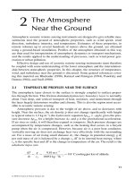
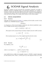
kinds of platforms. These algorithms, which treat a hyperspectral image as an image
cube made up of spatially arranged pixel vectors [18, 22, 12] (see Figure 18.1),
exhibit regular data access patterns and inherent data parallelism across both pixel
vectors(coarse-grainedpixel-levelparallelism) and spectralinformation (fine-grained
spectral-level parallelism). As a result, they map nicely to massively parallel systems
made up of commodity CPUs (e.g., Beowulf clusters) [20]. Unfortunately, these
systems are generally expensive and difficult to adapt to onboard remote sensing data
processing scenarios, in which low-weight integrated components are essential to
reduce mission payload. Conversely, the compact size and relative low cost are what
make modern GPUs appealing to onboard data processing.
The rest of thischapter isorganizedas follows.Section 18.2 begins with an overview
of the traditional rendering pipeline and eventually goes over the structure of modern
Width
Bands
Pixel Vector
Height
Figure 18.1 A hyperspectral image as a cube made up of spatially arranged pixel
vectors.
© 2008 by Taylor & Francis Group, LLC
414 High-Performance Computing in Remote Sensing
GPUs in detail. Section 18.3, in turn, covers the GPU programming model. First,
it introduces an abstract stream programming model that simplifies the mapping of
image processing applications to the GPU. Then it focuses on describing the essential
code transformations and algorithm trade-offs involved in this mapping process. After
this comprehensive introduction, Section 18.4 describes the Automatic Morpholog-
ical Endmember Extraction (AMEE) algorithm and its mapping to a modern GPU.
Section 18.5 evaluates the proposed GPU-based implementation from the viewpoint
of both endmember extraction accuracy (compared to other standard approaches) and
parallel performance. Section 18.6 concludes with some remarks and provides hints
at plausible future research.

18.2 Architecture of Modern GPUs
This section provides background on the architecture of modern GPUs. For this
introduction, it is useful to begin with a description of the traditional rendering
pipeline [8, 16], in order to understand the basic graphics operations that have to
be performed. Subsection 18.2.1 starts on the top of this pipeline, where data are fed
from the CPU to the GPU, and work their way down through multiple processing
stages until a pixel is finally drawn on the screen. It then shows how this logical
pipeline translates into the actual hardware of a modern GPU and describes some
specific details of the different graphics cards manufactured by the two major GPU
makers, NVIDIA and ATI/AMD. Finally, Subsection 18.2.2 outlines recent trends in
GPU design.
18.2.1 The Graphics Pipeline
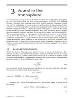
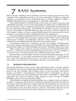
Figure 18.2 shows a rough description of the traditional 3D rendering pipeline. It
consists of several stages, but the bulk of the work is performed by four of them:
vertex-processing (vertex shading), geometry, rasterization, and fragment-processing
(fragment shading). The rendering process begins with the CPU sending a stream of
vertex from a 3D polygonal mesh and a virtual camera viewpoint to the GPU, using
some graphics API commands. The final output is a 2D array of pixels to be displayed
on the screen.
In the vertex stage the 3D coordinates of each vertex from the input mesh are trans-
formed (projected) onto a 2D screen position, also applying lighting to determine their
colors. Once transformed, vertices are grouped into rendering primitives, such as tri-
angles, and scan-converted by the rasterizer into a stream of pixel fragments. These
fragments are discrete portions of the triangle surface that correspond to the pixels of
the rendered image. The vertex attributes, such as texture coordinates, are then inter-
polated across the primitive surface storing the interpolated values at each fragment.
In the fragment stage, the color of each fragment is computed. This computation
usually depends on the interpolated attributes and the information retrieved from the
© 2008 by Taylor & Francis Group, LLC
Real-Time Onboard Hyperspectral Image Processing 415

Vertex
Stream
Proyected
Vertex
Stream
Fragment
Stream
Colored
Fragment
Stream
ROB
Memory
Fragment
Stage
Rasterization
Vertex
Stream
Figure 18.2 3D graphics pipeline.
© 2008 by Taylor & Francis Group, LLC
© 2008 by Taylor & Francis Group, LLC
416 High-Performance Computing in Remote Sensing
Vertex
Stage
Geometry
Stage
Fragment
Stage
Frag
Proc
HierarchicalZ

Rasterization
Triangle Setup
Clipping
Primitive Assembly
Vertex
Proc
Vertex
Proc
Vertex Fetch
Frag
Proc
Frag
Proc
ROP ROP
Memory
Controller
Memory
Controller
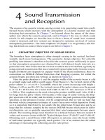
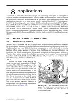
Figure 18.3 Fourth generation of GPUs block diagram. These GPUs incorporate
fully programmable vertexes and fragment processors.
graphics card memory by texture lookups.
1
The colored fragments are sent to the ROP
stage,
2
where Z-buffer checking ensures only visible fragments are processed further.
Those partially transparent fragments are blended with the existing frame buffer pixel.
Finally, if enabled, fragments are antialiazed to produce the ultimate colors.
Figure 18.3 shows the actual pipeline of a modern GPU. A detailed description
of this hardware is out of the scope of this book. Basically, major pipeline stages

corresponds 1-to-1 with the logical pipeline. We focus instead on two key features of
this hardware: programmability and parallelism.
r
Programmability. Until only a few years ago, commercial GPUs were
implemented using a hard-wired (fixed-function) rendering pipeline. However,
most GPUs today include fully programmable vertex and fragment stages.
3
The programs they execute are usually called vertex and fragment programs
1
This process is usually called texture mapping.
2
ROP denotes raster operations (NVIDIA’s terminology).
3
The vertex stage was the first one to be programmable. Since 2002, the fragment stage is also
programmable.
© 2008 by Taylor & Francis Group, LLC
Real-Time Onboard Hyperspectral Image Processing 417
(or shaders), respectively, and can be written using C-like high-level languages
such as Cg [6]. This feature is what allows for the implementation of non-
graphics applications on the GPUs.
r
Parallelism. The actual hardware of a modern GPU integrates hundreds of
physical pipeline stages per major processing stage to increase the through-
put as well as the GPU’s clock frequency [2]. Furthermore, replicated stages
take advantage of the inherent data parallelism of the rendering process. For
instance, the vertex and fragment processing stages include several replicated
units known as vertex and fragment processors, respectively.
4
Basically, the
GPU launches a thread per incoming vertex (or per group of fragments), which

is dispatched to an idle processor. The vertex and fragment processors, in turn,
exploit multithreading to hide memory accesses, i.e., they support multiple
in-flight threads, and can execute independent shader instructions in parallel as
well. For instance, fragment processors often include vector units that operate
on 4-element vectors (Red/Gree/Blue/Alpha channels) in an SIMD fashion.
Industry observers have identified different generations of GPUs. The descrip-
tion above corresponds to the fourth generation
5
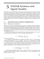
[7]. For the sake of completeness,
we conclude this subsection reproducing in Figure 18.4 the block diagram of two
representative examples of that generation: NVIDIA’s G70 and ATI’s Radeon R500
families. Obviously, there are some differences in their specific implementations, both
in the overall structure and in the internals of some particular stages. For instance, in
the G70 family the interpolation units are the first stage in the pipeline of each frag-
ment processor, while in the R500 family they are arranged in a completely separate
hardware block, outside the fragment processors. A similar thing happens with the
texture access units. In the G70 family they are located inside each fragment proces-
sor, coupled to one of their vector units [16, 2]. This reduces the fragment processors
performance in case of a texture access, because the associated vector unit remains
blocked until the texture data are fetched from memory. To avoid this problem, the
R500 family places all the texture access units together in a separate block.
18.2.2 State-of-the-art GPUs: An Overview
The recently released NVIDIA G80 families have introduced important new features,
which anticipate future GPU design trends. Figure 18.5 shows the structure of the
GeForce 8800 GTX, which is the most powerful G80 implementation introduced so
far. Two features stand out over previous generations:
r
Unified Pipeline. The G80’s pipeline only includes one kind of programmable
unit, which is able to execute three different kinds of shaders: vertex, geometry,
4

The number of fragment processors usually exceeds the number of vertex processors, which follows from
the general assumption that there are frequently more pixels to be shaded than vertexes to be projected
5
The fourth generation of GPUs dates from 2002 and begins with NVIDIA’s GeForce FX series and ATI’s
Radeon 9700 [7].
© 2008 by Taylor & Francis Group, LLC
418 High-Performance Computing in Remote Sensing
(a)
(b)
DRAM(s)DRAM(s)DRAM(s)
Memory
Partition
Memory
Partition
Fragment Crossbar
Z Cull
Shade Instruction Dispatch
Level 1
Texture Cache
Attribute
Interpolation
Vector
Unit 1
Fragment
Texture Unit
Vector and
Special-function
Unit 2
Temporary
registers

Output
L2 Tex
Cull/Clip/Setup
Host/FW/VTF
Memory
Partition
DRAM(s)
Memory
Partition
Texture Cache
Ultra-reading
Dispatch Processor
Quad
Pixel Shader
Core
Quad
Pixel Shader
Core
General Purpose Register Arrays
Z/Stencil Compare
Alpha/Fog
Render
Back-End
Compress
Decompress
Decompress
Multisample AA
Resolve
Blend
Color Buffer Cache

Quad
Pixel Shader
Core
Hierarchical
Z Test
Z/Stencil Buffer Cache
Pixel
Shader
Engine
Vertex
Shader
Engine
Vertex Data
8 Vertex Shader Processors
Backface Cull
Clip
Perspective Divide
Viewport Transform
Interpolators
Geometry Assembly
Rasterization
Texture Units
Texture Address
AlUs
Setup Engine
Vector ALU 2
Vector ALU 1
Scalar
ALU 1
Scalar

ALU
2
Figure 18.4 NVIDIA G70 (a) and ATI-RADEON R520 (b) block diagrams.
© 2008 by Taylor & Francis Group, LLC
Real-Time Onboard Hyperspectral Image Processing 419
FB FB FB FB FB FB
L2L2L2L2L2L2
L1
L1 L1 L1 L1 L1 L1 L1
TA TA TA TA
TF TF TF TF
TF
SP
SP
SP
Setup/Rstr/ZCull
Pixel read Issue
read Processor
Geom read Issue
Vtx read Issue
Input Assembler
Host
SP
SP
SP
SP
SP
TF TF TF
Figure 18.5 Block diagram of the NVIDIA’s Geforce 8800 GTX.
and fragment. This design reduces the number of pipeline stages and changes

the sequential flow to be more looping oriented. Inputs are fed to the top of
the unified shader core, and outputs are written to registers and then fed back
into the top of the shader core for the next operation. This unified architecture
promises to improve the performance for those programs dominated by only
one type of shader, which would otherwise be limited by the number of specific
processors available [2].
r
Scalar Processors. Another important change introduced in the NVIDIA’s G80
family over previous generations is the scalar nature of the programmable units.
In previous architectures both the vertex and fragment processors had SIMD
(vector) functional units, which were able to operate in parallel on the different
components of a vertex/fragment (e.g., the RGBA channels in a fragment).
However, modern shaders tend to use a mix of vector and scalar instructions.
Scalar computations are difficult to compile and schedule efficiently on a vector
pipeline. For this reason, NVIDIA’s G80 engineers decided to incorporate only
scalar units, called Stream Processors (SPs), in NVIDIA parlance [2]. The
GeForce 8800 GTX includes 128 of these SPs driven by a high-speed clock,
6
which can be dynamically assigned to any specific shader operation. Overall,
thousands of independent threads can be in flight in any given instant.
SIMD instructions can be implemented across groupings of SPs in close proximity.
Figure 18.5 highlights one of these groups with the associated Texture Filtering (TF),
Texture Addressing (TA), and Cache units. Using dedicated units for texture access
(TA) avoids the blocking problem of previous NVIDIA generations mentioned above.
6
The SPs are driven by a high-speed clock (1.35 GHz), separated from the core clock (575 MHz) that
drives the rest of the chip.
© 2008 by Taylor & Francis Group, LLC
420 High-Performance Computing in Remote Sensing
In summary, GPU makers will continue the battle for dominance in the consumer

gaming industry, producing a competitive environment with rapid innovation cycles.
New features will constantly be added to next-generation GPUs, which will keep de-
livering outstanding performance-per-dollar and performance-per-square millimeter.
Hyperspectral imaging algorithms fit relatively well with the programming environ-
ment the GPU offers, and can benefit from this competition. The following section
focuses on this programming environment.
18.3 General Purpose Computing on GPUs
For non-graphics applications, the GPU can be better thought of as a stream co-
processor that performs computations through the use of streams and kernels.A
stream is just an ordered collection of elements requiring similar processing, whereas
kernels are data-parallel functions that process input streams and produce new output
streams. For relatively simple algorithms this programming model may be easy to use,
but for more complex algorithms, organizing an application into streams and kernels
could prove difficult and require significant coding efforts. A kernel is a data-parallel
function, i.e., its outcome must not depend on the order in which output elements
are produced, which forces programmers to explicitly expose data parallelism to the
hardware.
This section illustrates how to map an algorithm to the GPU using this model. As an
illustrative example we have chosen the 2D Discrete Wavelet Transform (2D-DWT),
which has been used in the context of hyperspectral image processing for principal
component analysis [9], image fusion [15, 24], and registration [17] (among others).
Despite its simplicity, the comparison between the GPU-based implementations of the
popular Lifting(LS) and Filter-Bank (FBS) schemes ofthe DWT allows usto illustrate
some of the algorithmic trade-offs that have to be considered. This section begins with
the basic transformations that convert loop nests into an abstract stream programming
model. Eventually it goes over the actual mapping to the GPU using standard 3D
graphics API and describes the structure of the main program that orchestrates kernel
execution. Finally, it introduces a compact C++ GPU framework that simplifies this
mapping process, hiding the complexity of 3D graphics APIs.
18.3.1 Stream Programming Model

Our stream programmingmodel focuses on data-parallel kernels that operateon arrays
using gather operations, i.e., operations that read from random locations in an input
array. Storing the input and output arrays as textures, this kind of kernel can be easily
mapped to the GPU using fragment programs.
7
The following subsections illustrates
how to identify this kind of kernel and map them efficiently to the GPU.
7
Scatter operations write into random locations of a destination array. They are also common in certain
applications, but fragment programs only support gather operations.
© 2008 by Taylor & Francis Group, LLC
Real-Time Onboard Hyperspectral Image Processing 421
18.3.1.1 Kernel Recognition
The first step in the modeling process consists in identifying a set of potential kernels.
Specifically, we want to partition the target algorithm into a set of code blocks tagged
as kernel and non-kernel blocks. A kernel block is a parallel loop nest, i.e., a loop
nest that carries no data dependences, that can be modeled as Listing 1.
Listing 1 Kernel block. D
OUT
and D
IN
denote output and input arrays, respectively.
IDXdenotes index matrices for indirect array accesses
for all (i,j) do
D
OUT
1
[i, j] = F(i, j, D
IN
1

(IDX
11
(i, j)), );
D
OUT
2
[i, j] = F

(i, j, D
IN
1
(IDX

11
(i, j)), );

end for
The computations performed inside these loop nests define the kernels of our
stream model. The output streams are defined by the set of elements of the output
arrays D
OUT
that are written in the loop nest. Stream elements are arranged according
to their respective induction variables i and j. The input streams are defined by the
set of array elements read in the loop. Index arrays (IDX) allow for indirect access to
the input arrays D
IN
and eventually translate into texture coordinates. A non-kernel
block is whatever other construct that cannot be modeled as Listing 1, which accounts
for non-parallel loops and other sequential parts of the application such as control
flow statements, including the control flow of kernel blocks. These non-kernel blocks

will eventually be part of the main program that orchestrates and chains the kernel
blocks to satisfy data dependences.
Certain loop transformations could be useful for uncovering parallelism and en-
hancing kernel extraction. One of these is loop distribution (also know as loop fission),
which can be used for splitting a loop nest that does not match listing 1 into smaller
loop nests that do match that pattern.
The horizontal lifting algorithm helps us to illustrate this transformation. The
conventional implementation of LS shown in Listing 2 contains loop-carried flow
dependences and cannot be run in parallel. However, we can safely transform the
loop nest in Listing 2 into Listing 3 since it preserves all the data dependences of the
original code.
8
Notice that the transformed nested loops are free of loop-carried data
dependences and match our definition of a kernel block.
In general, this transformation can also be useful to restructure existing loop nests
in order to separate potentially parallel code (kernel blocks) from code that must
be sequentialized (non-kernel blocks). Nevertheless, it must be applied judiciously
since loop distribution results into finer granularity, which may deteriorate tempo-
ral locality and increase the overhead caused by kernel setup
9
and synchronization:
8
Loop distribution is a safe transformation when all the data dependences point forward [14].
9
Every kernel launch incurs a certain fixed CPU time to set up and issue the kernel on the GPU.
© 2008 by Taylor & Francis Group, LLC
422 High-Performance Computing in Remote Sensing
Distribution converts loop-independent and forward-carried dependences into depen-
dences between kernels, which forces kernel synchronization and reduces kernel level
parallelism. In fact, loop fusion, which performs the opposite operation, i.e., it merges

multiple loops into a single loop, may be beneficial when it creates a larger kernel
that still fits Listing 1.
Returning to our example, we are able to identify six kernels in the transformed
code, one for each loop nest. All of them read input data from two arrays and produce
one or two output streams (the first and the sixth loops produce two output streams,
whereas the others produce only one). As mentioned above, the loop-independent and
forward-carried dependences of the original LS loopnest convert into dependences
between these kernels, which forces synchronization between them to avoid race
conditions.
Obviously, more complex loop nests might require additional transformations to
uncover parallelism, such as loop interchange, scalar expansion, array renaming,
etc. [14]. Nevertheless, uncovering data parallelism is not enough to get an efficient
GPU mapping. The following subsection illustrates another transformation that deals
with specific GPU limitations.
Listing 2 Original horizontal LS loopnest. Specific boundary processing is not shown.
for i = 0toN − 1 do
for j = 0to(N − 1)/2 do
App[i,j] = A[i,2*j];
Det[i,j] = A[i,2*j+1];
end for
end for
{left boundary processing }
for i = 0toN − 1 do
for j = 0to(N − 6)/2 −1 do
Det[i,j+2] = Det[i,j+2] + alpha*(App[i,j+2] + App[i,j+3]);
App[i,j+2] = App[i,j+2] + beta *(Det[i,j+1] + Det[i,j+2]);
Det[i,j+1] = Det[i,j+1] + gamma*(App[i,j+1] + App[i,j+2]);
App[i,j+1] = App[i,j+1] + delta*(Det[i,j] + Det[i,j+1]);
Det[i,j] = Det[i,j]/phi;
App[i,j] = App[i,j]*phi;

end for
end for
{left boundary processing }
18.3.1.2 Platform-Dependent Transformations
Once we have uncovered enough data parallelism and extracted the initial kernels and
streams, we have to perform some additional transformations to efficiently map the
stream model to the target GPU.
© 2008 by Taylor & Francis Group, LLC
Real-Time Onboard Hyperspectral Image Processing 423
One of those transformations is branch removal. Although some GPUs tolerate
branches, they normally reduce performance, hence eliminating conditional sen-
tences from the kernel loops previously detected that would be useful. In some cases,
removing the branch from the kernel loop body transfers the flow control to the main
program, which will select between kernels based on a condition.
Listing 3Transformed horizontal LS loopnests. The original loop has been distributed
to increase kernel extraction. Specific boundary processing is not shown.
for i = 0toN − 1 do
for j = 0to(N − 1)/2 do
App[i,j] = A[i,2*j];
Det[i,j] = A[i,2*j+1];
end for
end for
{left boundary processing }
for i = 0toN − 1 do
for j = 0to(N − 6)/2 −1 do
Det[i,j+2] = Det[i,j+2] + alpha*(App[i,j+2] + App[i,j+3]);
end for
end for
for i = 0toN − 1 do
for j = 0to(N − 6)/2 −1 do

App[i,j+2] = App[i,j+2] + beta *(Det[i,j+1] + Det[i,j+2]);
end for
end for
for i = 0toN − 1 do
for j = 0to(N − 6)/2 −1 do
Det[i,j+1] = Det[i,j+1] + gamma*(App[i,j+1] + App[i,j+2]);
end for
end for
for i = 0toN − 1 do
for j = 0to(
N − 6)/2 −1 do
App[i,j+1] = App[i,j+1] + delta*(Det[i,j] + Det[i,j+1]);
end for
end for
for i = 0toN − 1 do
for j = 0to(N − 6)/2 −1 do
Det[i,j] = Det[i,j]/phi;
App[i,j] = App[i,j]*phi;
end for
end for
{right boundary processing }
© 2008 by Taylor & Francis Group, LLC
424 High-Performance Computing in Remote Sensing
Listing 4, which sketches the FBS scheme of the DWT, illustrates a common
example, where branch removal provides significant performance gains. The second
loop (the j loop) matches Listing 1, but its body includes two branches associated
with the non-parallel inner loops (the k loops). These inner loops perform a reduction
whose outcomes are finally writtenon theoutput arrays. In this example, the inner loop
bounds are known at compile time. Therefore, they can be fully unrolled (actually this
is what NVIDIA’s Cg compiler generally does). However, removing loop branches

through unrolling is not always possible since there is a limit on the number of
instructions per kernel.
Listing 4 Original horizontal FBS loopnest. Specific boundary processing is not
shown.
{left boundary processing }
for i = 0toN − 1 do
for j = 2to(N − 6)/2 do
aux=0;
for k = 0toLENGTH
H do
aux=aux+h[k]*A[i,2 ∗ j − LENGTH
H/2 + k];
end for
App[i, j] = aux;
aux=0;
for k = 0toLENGTH
G do
aux=aux+g[k]*A[i,2 ∗ j − LENGTH
G/2 + k];
end for
Det[i, j] = aux;
end for
end for
{right boundary processing }
Loop distribution can also be required to meet GPU render target (number of
shader outputs) constraints. Some GPUs do not permit several render targets, i.e.,
output streams, in a fragment shader, or have a limit on the number of targets. For
instance, if we run LS on a GPU that only allows one render target, the first and
sixth loops in Listing 3 have to be distributed into two kernels, each one writing to a
different array. Notice that in this case, unlike the previous distribution that converts

Listing 2 into Listing 3, the new kernels can run in parallel, since both loopnests are
free of dependences.
Finally, GPU memory constraints have to be considered. Obviously, we need to
restrict the size of the kernel loop nests so that the amount of elements accessed in
these loops fits into this memory. This is usually achieved by tiling or strip-mining
the kernel loop nests. For instance, if the input array in the FBS algorithm is too
large, we should tile the loops in Listing 4. Listing 5 shows a transformed FBS code
after applying loop tiling and distributing the loops in order to meet render target
© 2008 by Taylor & Francis Group, LLC
Real-Time Onboard Hyperspectral Image Processing 425
constraints. The external loops (ti, tj) have been fused to improve temporal locality,
i.e., the two filter loops have been tiled in a way that both kernels read from the same
data in every iteration of the external loops. This way, we reduce memory transfers
between the GPU and the main memory, since data have to be transferred to the GPU
only once.
Listing 5 Transformed horizontal FBS loopnest. The original loopnest has been tiled
and distributed to meet memory and render target constraints (assuming only one
render target is possible). Specific boundary processing is not shown.
{left boundary processing }
for ti = 0to(N − 1)/TI do
for tj = 2to((N − 6)/2)/TJdo
for i = ti ∗ TI to (ti +1) ∗ TI−1 do
for j = tj∗ TJto (tj + 1) ∗ TJ− 1 do
aux=0;
for k = 0toLENGTH
H do
aux=aux+h[k]*A[i,2 ∗ j − LENGTH
H/2 + k];
end for
App[i, j] = aux;

end for
end for
for i = ti ∗ TI to (ti +1) ∗ TI−1 do
for j = tj∗ TJto (tj + 1) ∗ TJ− 1 do
aux=0;
for k = 0toLENGTH
G do
aux=aux+g[k]*A[i,2 ∗ j − LENGTH
G/2 + k];
end for
Det[i, j] = aux;
end for:kernel-block
end for
end for
end for
{right boundary processing }
Loop tiling is also useful to optimize cache locality. GPU texture caches are heavily
optimized for graphics rendering. Therefore, given that the reference patterns of
GPGPU applications usually differ from those for rendering, GPGPU applications
can lack cache performance. We do know that these caches are organized to capture
2D locality [10], but we do not know their exact specifications today, as they are
not released by GPU makers. This lack of information complicates the practical
application of tiling since the structure of the target memory hierarchy is the principal
factor in determining the tile size. Therefore, some sort of memory model or empirical
tests will be needed to make this transformation useful.
© 2008 by Taylor & Francis Group, LLC
426 High-Performance Computing in Remote Sensing
H
Horizontal
DWT

Original
Image
G
Horizontal
DWT
1/Phi
Phi
DeltaGammaBetaAlpha
Odd
Even
Original
Image
Figure 18.6 Stream graphs of the GPU-based (a) filter-bank (FBS) and (b) lifting
(LS) implementations.
18.3.1.3 The 2D-DWT in the Stream Programming Model
Figures 18.6(a) and 18.6(b) graphically illustrate the implementation of the two
DWT algorithms in the stream programming model. These stream graphs have been
extracted from the sequential code applying the previous transformations. For the
FBS we only need two kernels, one for each filter. Furthermore, these kernels can be
run in parallel (without synchronization) as both write on different parts of the output
arrays and do not depend on the results of each other. On the other hand, the depen-
dences between LS steps translate into a higher number of kernels, which results in
finer grain parallelism (each LS step is performed by a different kernel) and explicit
synchronization barriers between them to avoid race conditions.
These algorithms also allow us to highlight the parallelism versus complexity
trade-off that developers usually face. Theoretically, LS requires less arithmetic op-
erations than its FBS counterpart, down to one half depending on the type and length
of the wavelet filter [4]. In fact, LS is usually the most efficient strategy in general-
purpose microprocessors [13]. However, its FBS fits better the programming environ-
ment the GPU offers. In practice, performance models or empirical tests are needed

to evaluate these kinds of trade-offs.
18.3.2 Stream Management and Kernel Invocation
As mentioned above, kernel programs can be written in high-level C-like languages
such as Cg [7]. However, we must still use a 3D graphics API, such as OpenGL,
to organize data into streams, transfer those data streams to and from the GPU as
2D textures, upload kernels, and perform the sequence of kernel calls dictated by
the application flow. In order to illustrate these concepts, Figure 18.8 shows some of
the OpenGL commands and the respective Cg code that performs one lifting step (the
ALPHA step). The following subsections describe this example code in detail.
© 2008 by Taylor & Francis Group, LLC
Real-Time Onboard Hyperspectral Image Processing 427
Initial
Data
Array A
Produced
Streams
App Det
Figure 18.7 2D texture layout.
18.3.2.1 Mapping Streams to 2D Textures
In our programming model, the stream management is performed by allocating a
single 2D texture, large enough to pack all the input and output data streams (not
shown in Figure 18.8). Given that textures are made up of 4-channel elements,
knownas texels, different data-to-texel mappings arepossible. The most profitable one
depends on the operations being performed in the the kernel loops, since this mapping
determines the following key performance factors:
r
SIMD parallelism. As mentioned above, fragment processors usually have
vector units that process the four elements of a texel in a SIMD fashion.
r
Locality. Texel mapping influences the memory access behavior of the kernels

since fetching one texel only requires one memory access.
r
Automatic texture addressing. Texture mapping may also determine how
texture coordinates (addresses) are computed. If the number of texture
addresses needed by a kernel does not exceed the number of available hardware
interpolators, memory address calculations can be accelerated by hardware.
For the DWT, a 2D layout is an efficient mapping, i.e., packing two elements from
two consecutive rows of the original array into each texel. This layout permits all the
memory (texture) address calculations to be performed by the hardware interpolators.
Nevertheless, for the sake of simplicity we will consider a simpler texel mapping, in
which each texel contains only one array element, in the rest of this section.
Apart from the texel mapping, we should also define the size and aspect ratio of
the allocated 2D texture as well as the actual allocation of input and output arrays
within this texture. For example, Figure 18.7 illustrates these decisions for our DWT
implementations. We use a 2D texture twice as large as the original array. The initial
data (array A in Listing 3) are allocated on the top half of this texture, whereas
the bottom half will eventually contain the produced streams (the App and Det in
Listing 3) .
© 2008 by Taylor & Francis Group, LLC
428 High-Performance Computing in Remote Sensing
18.3.2.2 Orchestrating Memory Transfers and Kernel Calls
With data streams mapped onto 2D textures, our programming model uses the GPU
fragment processors to execute kernels (fragment shaders) over the stream elements.
In an initialization phase, the main program uploads these fragment shaders into the
graphics hardware. Later on, they are invoked on demand according to the application
flow.
10
To invoke a kernel, the size of the output stream must be defined. This definition
is done by drawing a rectangle that covers the region of pixels matching the output
stream. The glVertex2f OpenGL commands define the vertex coordinates of this rect-

angle, i.e., they delimit the output area, which is equivalent to specifying the kernel
loop bounds. The vertex processor and the rasterizer transform the rectangle to a
stream of fragments, which are then processed by the active fragment program.
Among the attributes of the generated fragment, we find hardware interpolated 2D
texture coordinates, which are used as indexes to fetch the input data associated to that
fragment.
11
To delimit those input areas, the glMultiTexCoord2fvARB OpenGL com-
mands assign texture coordinates at each vertex of the quad. In our example, we have
three equal-sized input areas, which partially overlap with each other, since we must
fetch three different elements (Det[i][j], App[i][j] and App[i][j+1]) per output value.
In the example, both the input and output areas have the same size and aspect ratio,
but they can be different. For instance, the FBS version takes advantage of the linear
interpolation to perform downsampling by defining input areas twice as wide as the
output one.
As mention above, there is a limit on the number of texture coordinates (per frag-
ment) that can be hardware interpolated, which depends on the target GPU. As long
as the number of input elements that we must fetch per output value is lower than this
limit (as in the example), memory addresses are computed by hardware. Otherwise,
texture coordinates must be computed explicitly on the fragment program.
Finally, synchronization between consumers and producers is performed using the
OpenGL glFinish() command. This function does not return until the effects of all pre-
viously invoked GL commands are completed and it can be seen as a synchronization
barrier. In the example, we need barriers between every lifting step.
18.3.3 GPGPU Framework
As shown in the previous section, in order to exploit the GPU following a stream
programming model, we have to deal with the many abstraction layers that the sys-
tem introduces to ease the access to graphics hardware in graphics applications. As
we can observe in Figure 18.8, these layers do nothing but cloud the resources we
want to use. Therefore, it is useful for us to build some abstraction layers that bring

together our programming model and the graphics hardware, so we can move away
10
In our example, Active fp(Alpha fp) enables the Alpha fp fragment program. Kernels always operate on
the active texture, which is selected byActive
texture.
11
This operation is also known as texture lookup in graphics terminology.
© 2008 by Taylor & Francis Group, LLC
Real-Time Onboard Hyperspectral Image Processing 429
STREAM FLOW MODEL
Horizontal
DWT
1/Phi
Phi
Delta
Gamma
Beta
Alpha
Even
Odd
Original
Image
Input Stream:
Fragments
to be Shaded
Input Streams:
Texture Elements
Fetched
Output Streams:
Shaded Fragments

Alpha_fp
INITIAL
DATA
RESULTS
t5
t0
t6 t1 t7
t2
t9 t4 t8 t3
Alpha_fp
Alpha Stage C code
CPU Driving Program
Figure 18.8 Mapping one lifting step onto the GPU.
the graphics API, worthless – even harmful – in our case. In this section, we present
the API of the framework we have been using in our research to clarify how we can
easily utilize a graphics card to implement the stream flow models developed for our
target algorithms.
18.3.3.1 The Operating System and the Graphics Hardware
In an operating system, we find that access to the graphics hardware implies going
through a series of graphics libraries and extensions to the windowing system. First
of all, we have to install a driver for the graphics card, which exports an API to the
windowing system. Then, the windowing system exports an extension for initializing
© 2008 by Taylor & Francis Group, LLC
430 High-Performance Computing in Remote Sensing
VMEN
GPU
GLX
Open GL
GPGPU Framework
Linux kernal

X Window
Graphics
Card Driver
Execution
Resources Access
Video
Memory Access
Memory Manager
GPUStream
GPUKernel
VMENGPU
Setup
GPGPU
GPGPU
Figure 18.9 Implementation of the GPGPU Framework.
our graphics card, so it can be used through the common graphics libraries – like
OpenGLor DirectX – that providehigher level primitives for 3D graphics applications.
In GNU/Linux (see Figure 18.9(a)), the driver is supplied by the graphics card’s
manufacturer, the windowing system, is the X Window System, and the graphics
library is OpenGL, which can be initialized through the GLX extension. Our GPGPU
framework hides the graphics-related complexity, i.e., the X Window System, the
GLX, and the OpenGL library.
Figure 18.9(b) illustrates the software architecture of the GPGPU framework we
implement. It consists of three classes: GPUStreams, GPUKernels, and a GPGPU
static class for GPU and video memory managing.
The execution resources are handled through the GPUKernel class, which repre-
sents our execution kernels. We can control the GPGPU mode through the GPGPU
class and transfer data to and from the video memory using the GPUStream class. This
© 2008 by Taylor & Francis Group, LLC
Real-Time Onboard Hyperspectral Image Processing 431

TABLE 18.1
GPGPU Class Methods
GPGPU
method input params output params
initialize width, height, chunks (void)
getGPUStream width, height GPUStream*
freeGPUStream GPUStream* (void)
waitForCompletion (void) (void)
way, we provide a stream model friendly API that allows us to directly implement the
stream flow models of our target applications, avoiding most of the graphics issues.
18.3.3.2 The GPGPU Framework
The static class GPGPU allows us to initialize and finalize the GPGPU mode and
wait for the GPU to complete any kernel execution or data transference in progress.
In addition, it incorporates a memory manager to allocate and free video memory.
Two possible implementations of the memory manager are possible: a multi-texture
or a single-texture model. In the former, the memory manager allocates the different
streams as different textures that provide a noticeableamount ofstreams (upto sixteen)
that can be managed at a time in our kernels. In addition, all these textures can be
independently accessed using the results from the eight hardware interpolators, i.e.,
a single coordinate references one element on each stream as the texture coordinates
are shared among them.
On the other hand, the single-texture model allocates all the streams as different
regions of a single 2D texture. This model limits the amount of memory that can be
managed.
12
Furthermore, each hardware-interpolated texture coordinate can only be
used to access one element in one stream, i.e., one element in the texture. However,
it is always possible to compute extra coordinates in the fragment shader. Despite
of all these limitations, a single-texture model has a definitive advantage: a unified
address space. This allows us to identify a stream by its location in the unified address

space and store this location as data in other streams, i.e., we can use pointers to
streams. On the contrary, this is not possible in a multi-texture model since we cannot
store a texture identifier as data. This limitation in the multi-texture model makes it
difficult to dereferencing streams based on the output of previous kernels (it may be
very inefficient or even impossible).
Because of the benefits of the single address space, we decided to implement
the memory manager following the single-texture model, using a first-fit policy to
allocate the streams on the texture. The interface of the GPGPU class is shown in
Table 18.1.
12
The maximum size for a texture that OpenGL allows us to allocate is 4096 × 4096 texels, so we are
limited to 256MB of video memory (4096 ×4096 × 4(RGBA)×4(floating point elements)).
© 2008 by Taylor & Francis Group, LLC
432 High-Performance Computing in Remote Sensing
TABLE 18.2
GPUStream Class Methods
GPUStream
method input params output params
writeAll float* (void)
write x
0
, y
0
, width, height, float* (void)
readAll (void) float*
read x
0
, y
0
, width, height float*

setValue float (void)
getSubStream x
of f
, y
of f
, width, height GPUStream*
getX/getY (void) int
getWidth/getHeight (void) int
Once the GPGPU mode has been set up, we have access to the video memory
through GPUStream objects, whose methods are shown in Table 18.2. We can trans-
fer data between the main memory and the GPUStreams by using the read[All]
and write[All] methods. getSubStream allow, us to obtain a displaced reference to a
stream: We can specify an off-set from the original position of the stream in memory
(x
of f
, y
of f
), and the width and height of the new stream. This way, we can use differ-
ent regions of the same stream as different streams, as the example in Figure 18.10
illustrates.
Our kernels, written in Cg [7], are managed in the application through the GPUK-
ernel objects, whose methods are shown in Table 18.3. We can use these objects to
run kernels on different streams, which are passed as parameters. Apart from streams,
we can also pass constant arguments through the set[Local}Named]Param method.
The launch method is a non-blocking version of run.
These three classes (GPGPU, GPUKernel, and GPUStream) abstract all the basic
functionality required to map applications in the stream programming model to the
GPU. For instance, Listing 6 shows the C++ code for the implementation of the
algorithm in Figure 18.10, while Listings 7 and 8 show the Cg codes of the kernels
used in this example.

DCDC
B = A + D;
C = A – D;
A = S.getSubStream(0, 0, 4, 2);
C = S.getSubStream(0, 2, 4, 2);
D = S.getSubStream(4, 2, 4, 2);
B = S.getSubStream(4, 0, 4, 2);
B
SS
26
42
23
3130
22
40
2422
38
21
2928
20
36
203210
89
1110
–20–20–20–20
–20–20
–20
–20
ABA
S

0
1234567
8 9 10 11 12 13 14 15
16 17 18 19 20 21 22 23
24
25 26 27 28 29 30 31
0
1234567
8 9 10 11 12 13 14 15
16 17 18 19 20 21 22 23
24
25 26 27 28 29 30 31
Figure 18.10 We allocate a stream S of dimension 8 × 4 and initialize its content
to a sequence of numbers (from 0 to 31). Then, we ask four substreams dividing the
original stream into four quadrants (A, B, C, and D). Finally, we add quadrants A
and D and store the result in B, and we substract D from A and store the result in C.
© 2008 by Taylor & Francis Group, LLC
Real-Time Onboard Hyperspectral Image Processing 433
TABLE 18.3
GPUKernel Class Methods
GPUKernel
method input params output params
setNamedParam char* name, StreamElement (void)
setLocalParam int pos, StreamElement (void)
launch GPUStream*, GPUStream*
run GPUStream*, GPUStream*
Listing 6 C++ Main program for the example in Figure 18.10.
#include "GPGPU.h"
int main( )
{

// Allocate enough video memory
GPGPU::Initialize( 128, 128, 1 );
// Allocate the main stream
GPUStream∗ S = GPGPU::getGPUStream( 8, 4 );
float data[32];
for( int i=0;i< 32; i++ ) data[i] = i;
// Write the initial data to the stream
S
>writeAll( data );
// Create 4 streams as references to four quadrants of S
GPUStream∗ A=S
>getSubStream( 0, 0, 4, 2 );
GPUStream∗ B=S
>getSubStream( 4, 0, 4, 2 );
GPUStream∗ C=S
>getSubStream( 0, 2, 4, 2 );
GPUStream∗ D=S
>getSubStream( 4, 2, 4, 2 );
// Load kernels for addition and substraction
GPUKernel∗ add( "add.cg" );
GPUKernel∗ sub( "sub.cg" );
// Run them in parallel
add
>launch( A, D, B ); // Asynchronous
sub
>run( A, D, C ); // Synchronous
GPGPU::Finalize( );
}
© 2008 by Taylor & Francis Group, LLC
434 High-Performance Computing in Remote Sensing

Listing 7 Cg code for an addition kernel, which takes two streams and adds them.
void add( in float2 s1 coord : TEXCOORD0,
in float2 s2
coord : TEXCOORD1,
out float s1
plus s2 : COLOR,
const uniform samplerRECT mem )
{
// We dereference the corresponding stream elements
float s1 = texRECT( mem, s1
coord );
float s2 = texRECT( mem, s2
coord );
// We add them and return the result
s1
plus s2=s1+s2;
}
Listing 8 Cg code for a substraction kernel, which takes two streams and substract
them.
void sub( in float2 s1 coord : TEXCOORD0,
in float2 s2
coord : TEXCOORD1,
out float s1
minus s2 : COLOR,
const uniform samplerRECT mem )
{
// We dereference the corresponding stream elements
float s1 = texRECT( mem, s1
coord );
float s2 = texRECT( mem, s2

coord );
// We substract s2 from s1 and return the result
s1
minus s2=s1 s2;
}
18.4 Automatic Morphological Endmember Extraction on GPUs
This section develops a GPU-based implementation of the Automatic Morphological
Endmember Extraction (AMEE) algorithm following the design guidelines outlined
above. First, we provide a high-level overview of the algorithm, and then we discuss
the specific aspects about its implementation on a GPU.
18.4.1 AMEE
Let us denote by f a hyperspectral data set defined on an N-dimensional (N-D) space,
where N is the number of channels or spectral bands. The main idea of the AMEE
algorithm is to impose an ordering relation in terms of spectral purity in the set of
© 2008 by Taylor & Francis Group, LLC
Real-Time Onboard Hyperspectral Image Processing 435
pixel vectors lying within a spatial search window or structuring element around each
image pixel vector [21]. To do so, we first define a cumulative distance between one
particular pixel f(x, y), i.e., an N-D vector at discrete spatial coordinates (x, y), and
all the pixel vectors in the spatial neighborhood given by B (B-neighborhood) as
follows [18]:
D
B
(f(x, y)) =

(i, j)∈Z
2
(B)
Dist(f(x, y), f(i, j)) (18.1)
where (i, j) are the spatial coordinates in the B-neighborhood discrete domain, repre-

sented by Z
2
(B), and Dist is a pointwise distance measure between two N-D vectors.
The choice of Dist is a key topic in the resulting ordering relation. The AMEE algo-
rithm makesuse of the spectral anglemapper (SAM), astandard measure inhyperspec-
tral analysis [3]. For illustrative purposes, let us assume that s
i
= (s
i1
, s
i2
, ,s
iN
)
T
and s
j
= (s
j1
, s
j2
, ,s
jN
)
T
are two N-D signatures. Here, the term ‘spectral sig-
nature’ does not necessarily imply ‘pixel vector’ and hence spatial coordinates are
omitted from the two signatures above, although the following argumentation would
be the same if pixel vectors were considered. The SAM between s
i

and s
j
is given by
SAM(s
i
, s
j
) = cos
−1
(s
i
· s
j
/s
i
·s
j
) (18.2)
It should be noted that SAM is invariant in the multiplication of input vectors by
constants and, consequently, is invariant to unknown multiplicative scalings that may
arise due to differences in illumination and sensor observation angles.
In contrast, SID is based on the concept of divergence and measures thediscrepancy
of probabilistic behaviors between two spectral signatures. If we assume that s
i
and s
j
are nonnegative entries, then two probabilistic measures can be respectively defined
as follows:
M[s
ik

] = p
k
= s
ik
/
N

l=1
s
il
M[s
jk
] = q
k
= s
jk
/
N

l=1
s
jl
(18.3)
Using the above definitions, the self-information provided by s
j
for band l is given
by I
l
(s
j

) =−log q
l
. We can further define the entropy of s
j
with respect to s
i
by
D(s
i
s
j
) =
N

l=1
p
l
D
l
(s
i
s
j
)
=
N

l=1
p
l

(I
l
(s
j
) − I
l
(s
i
)) =
N

l=1
p
l
log(p
l
/q
l
)
(18.4)
By means of equation (18.4), SID is defined as follows:
SID(s
i
, s
j
) = D(s
i
s
j
) + D(s

j
s
i
) (18.5)
With the above definitions in mind, we provide below a step-by-step description
of the AMEE algorithm that corresponds to the implementation used in [19]. The
© 2008 by Taylor & Francis Group, LLC