Challenges and Paradigms in Applied Robust Control Part 5 doc
Bạn đang xem bản rút gọn của tài liệu. Xem và tải ngay bản đầy đủ của tài liệu tại đây (1.27 MB, 30 trang )
Robust Active Suspension Control for Vibration Reduction of Passenger's Body
109
dynamics. Varterasian & Thompson reported the seated human dynamics from a large
person to a small person(Varterasian & Thompson, 1977). Robust performance is verified by
supposition that such person sits in the vehicle. Figure 16 shows the frequency response
from vertical vibration of seat to vertical vibration of the head. Dot is 15 subjects' resonance
peak. In this section, three outstanding subjects' data of their report is modeled in the
vibration characteristic of vertical direction. The damper and spring were adjusted to
conform the passenger model and an experimental data. The characteristic of the passenger
model of three outstanding subjects are shown in Table 4.
k
p3
[N/m]
c
p3
[N/m/s]
Nominal model 960000 1120
Subject 1 1320000 1150
Subject 2 576000 960
Subject 3 960000 2550
Table 4. Difference of specifications
Nominal model Subject 1 Subject 2 Subject 3
10
0
10
1
10
-4
10
-3
10
-2
10
-1
PSD [(m/s
2
)
2
/Hz]
Frequency[Hz]
Fig. 17. PSD of vertical acceleration (Passenger 1’s head)
The numerical simulation is carried out on the same road surface conditions as the section
4.5.1. Figure 17 shows PSD of the vertical acceleration of the passenger 1’s head and Fig. 18
Challenges and Paradigms in Applied Robust Control
110
shows RMS value. In PSD of 7 Hz or more, RMS value of vertical acceleration of subject 1’s
head becomes higher than the nominal model. Moreover, RMS of subject 1 is the highest. On
the other hand, RMS of subjects 2 and 3 is reduced in comparison with the nominal model.
The physique of subject 1 differs from other subjects. When such a person sits, the specified
controller should be designed. From these results, the proposed method has robustness for
the passenger of the general physique.
100
100
104.6
96.1
97.7
97.1
92.5
112.1
40
50
60
70
80
90
100
110
120
130
140
Head 1 Head 2
RMS ratio to Nominal controller[%]
Nominal Subject 1 Subject 2 Subject 3
Fig. 18. RMS value of vertical acceleration of passenger 1’s head
5. Conclusion
This study aims at establishing a control design method for the active suspension system in
order to reduce the passenger's vibration. In the proposed method, a generalized plant that
uses the vertical acceleration of the passenger’s head as one of the controlled output is
constructed to design the linear
H
∞
controller. In the simulation results, when the actuating
force is limited, we confirmed that the proposed method can reduce the passenger's
vibration better than two methods which are not include passenger’s dynamics. Moreover,
the proposed method has robustness for the difference in passenger’s vibration
characteristic.
6. Acknowledgment
This work was supported in part by Grant in Aid for the Global Center of Excellence
Program for "Center for Education and Research of Symbiotic, Safe and Secure System
Design" from the Ministry of Education, Culture, Sport, and Technology in Japan.
7. References
Ikeda, S.; Murata, M.; Oosako, S. & Tomida, K. (1999). Developing of New Damping Force
Control System -Virtual Roll Damper Control and Non-liner
H
∞
Control-,
Transactions of the TOYOTA Technical Review, Vol.49. No.2, pp.88-93
Robust Active Suspension Control for Vibration Reduction of Passenger's Body
111
Kosemura, R.; Takahashi, M. & and Yoshida, K. (2008). Control Design for Vehicle Semi-
Active Suspension Considering Driving Condition,
Proceedings of the Dynamics and
Design Conference 2008
, 547, Kanagawa, Japan, September, 2008
Itagaki, N.; Fukao, T.; Amano, M.; Ichimaru, N.; Kobayashi, T. & Gankai, T. (2008). Semi-
Active Suspension Systems based on Nonlinear Control,
Proceedings of the 9th
International Symposium on Advanced Vehicle Control 2008
, pp. 684-689, Kobe, Japan,
October, 2008
Tamaoki, G.; Yoshimura, T. & Tanimoto, Y. (1996). Dynamics and Modeling of Human Body
Considering Rotation of the Head,
Proceedings of the Dynamics and Design Conference
1996
, 361, pp. 522-525, Fukuoka, Japan, August, 1996
Tamaoki, G.; Yoshimura, T. & Suzuki, K. (1998). Dynamics and Modeling of Human Body
Exposed to Multidirectional Excitation (Dynamic Characteristics of Human Body
Determined by Triaxial Vibration Test),
Transactions of the Japan Society of Mechanical
Engineers, Series C
, Vol.64, No.617, pp. 266-272
Tamaoki, G. & Yoshimura, T. (2002). Effect of Seat on Human Vibrational Characteristics,
Proceedings of the Dynamics and Design Conference 2002, 220, Kanazawa, Japan,
October, 2002
Koizumi, T.; Tujiuchi, N.; Kohama, A. & Kaneda, T. (2000). A study on the evaluation of ride
comfort due to human dynamic characteristics,
Proceedings of the Dynamics and
Design Conference 2000
, 703, Hiroshima, Japan, October, 2000 ISO-2631-1 (1997).
Mechanical vibration and shock–Evaluation of human exposure to whole-body
vibration -,
International Organization for Standardization ISO-5982 (2001). Mechanical
vibration and shock –Range of idealized value to characterize seated body
biodynamic response under vertical vibration,
International Organization for
Standardization
Oya, M.; Tsuchida, Y. & Qiang, W. (2008). Robust Control Scheme to Design Active
Suspension Achieving the Best Ride Comfort at Any Specified Location on
Vehicles,
Proceedings of the 9th International Symposium on Advanced Vehicle Control
2008
, pp.690-695, Kobe, Japan, October, 2008
Guglielmino, E.; Sireteanu, T.; Stammers, C. G.; Ghita, G. & Giuclea, M. (2008).
Semi-Active
Suspension Control -Improved Vehicle Ride and Road Friendliness
, Springer-Verlag,
ISBN- 978-1848002302, London
Okamoto, B. and Yoshida, K. (2000). Bilinear Disturbance-Accommodating Optimal Control
of Semi-Active Suspension for Automobiles,
Transactions of the Japan Society of
Mechanical Engineers, Series C
, Vol.66, No.650, pp. 3297-3304
Glover, K. & Doyle, J.C. (1988). State-space Formula for All Stabilizing Controllers that
Satisfy an
H
∞
-norm Bound and Relations to Risk Sensitivity, Journal of the Systems
and Control letters
, 11, pp.167-172
ISO-8608 (1995). Mechanical vibration -Road surface profiles - Reporting of measured data,
International Organization for Standardization
Rimel, A.N. & Mansfield, N.J. (2007). Design of digital filters for Frequency Weightings
Required for Risk Assessment of workers Exposed to Vibration,
Transactions of the
Industrial Health
, Vol.45, No.4, pp. 512-519
Challenges and Paradigms in Applied Robust Control
112
Varterasian, H. H. & Thompson, R. R. (1977). The Dynamic Characterristics of Automobiles
Seats with Human Occupants,
SAE Paper, No. 770249
6
Modelling and Nonlinear Robust Control of
Longitudinal Vehicle Advanced ACC Systems
Yang Bin
1
, Keqiang Li
2
and Nenglian Feng
1
1
Beijing University of Technology
2
Tsinghua University
China
1. Introduction
Safety and energy are two key issues to affect the development of automotive industry. For
the safety issue, the vehicle active collision avoidance system is developing gradually from a
high-speed adaptive cruise control (ACC) to the current low-speed stop and go (SG), and
the future research topic is the ACC system at full-speed, namely, the advanced ACC
(AACC) system. The AACC system is an automatic driver assistance system, in which the
driver's behavior and the complex traffic environment ranging are taken into account from
high-speed to low-speed. By combining the function of the high-speed ACC and low-speed
SG, the AACC system can regulate the relative distance and the relative velocity adaptively
between two vehicles according to the driving condition and the external traffic
environment. Therefore, not only can the driver stress and the energy consumption caused
by the frequent manipulation and the traffic congestion both be reduced effectively at the
urban traffic environment, but also the traffic flow and the vehicle safety will be improved
on the highway.
Taking the actual traffic environment into account, the velocity of vehicle changes regularly
in a wide range and even frequently under SG conditions. It is also subject to various
external resistances, such as the road grade, mass, as well as the corresponding impact from
the rolling resistance. Therefore, the behaviors of some main components within the power
transmission show strong nonlinearity, for instance, the engine operating characteristics,
automatic transmission switching logic and the torque converter capacity factor. In addition,
the relative distance and the relative velocity of the inter-vehicles are also interfered by the
frequent acceleration/deceleration of the leading vehicle. As a result, the performance of the
longitudinal vehicle full-speed cruise system (LFS) represents strong nonlinearity and
coupling dynamics under the impact of the external disturbance and the internal
uncertainty. For such a complex dynamic system, many effective research works have been
presented. J. K. Hedrick et al. proposed an upper+lower layered control algorithm
concentrating on the high-speed ACC system, which was verified through a platoon cruise
control system composed of multiple vehicles
[1-3]
. K. Yi et al. applied some linear control
methods, likes linear quadratic (LQ) and proportional–integral–derivative (PID), to design
the upper and lower layer controllers independently for the high-speed ACC system
[4]
. In
ref.[5], Omae designed the model matching control (MMC) vehicle high-speed ACC system
based on the H-infinity (H
inf
) robust control method. To achieve a tracking control between
Challenges and Paradigms in Applied Robust Control
114
the relative distance and the relative velocity of the inter-vehicles, A. Fritz proposed a
nonlinear vehicle model for the high-speed ACC system with four state variables in refs.[6,
7], and designed a variable structure control (VSC) algorithm based on the feedback
linearization. In ref. [8], J.E. Naranjo used the fuzzy theory to design a coordinate control
algorithm between the throttle actuator and the braking system. It has been verified on an
ACC and SG cruise system. Utilizing the model predictive control (MPC) method, D. Coron
designed an ACC control system for a SMART Car
[9]
. G. N. Bifulco applied the human
artificial intelligence to study an ACC control algorithm with anthropomorphic function
[10]
.
U. Ozguner investigated the impact of inter-vehicles communications on the performance of
vehicle cruise control system
[11]
. J. Martinez, et al. proposed a reference model-based
method, which has been applied to the ACC and SG system, and achieved an expected
tracking performance at full-speed condition
[12]
. Utilizing the idea of hierarchical design
method, P. Venhovens proposed a low-speed SG cruise control system, and it has been
verified on a BMW small sedan
[13]
. Y. Yamamura developed an SG control method based on
an existing framework of the ACC control system, and applied it to the SG cruise control
[14]
.
Focusing on the low-speed condition of the heavy-duty vehicles, Y. Bin et al. derived a
nonlinear model
[15, 16]
and applied the theory of nonlinear disturbance decoupling (NDD)
and LQ to the low-speed SG system
[17, 18]
.
In the previous research works, the controlled object (i.e. the dynamics of the controlled
vehicle) was almost simplified as a linear model without considering its own mass, gear
position and the uncertainty from external environment (likes, the change of the road
grade). Furthermore, the analysis of the disturbance from the leading vehicle’s acceleration/
deceleration was not paid enough consideration, which has become a bottleneck in limiting
the enhancement of the control performance. To summarize, based on a detailed analysis of
the impact from the practical high/low speed operating condition, the uncertainty of
complex traffic environment, vehicle mass, as well as the change of gear shifting to the
vehicle dynamic, an innovative LFS model is proposed in this study, in which the dynamics
of the controlled vehicle and the inter-vehicles are lumped together within a more accurate
and reasonable mathmatical description. For the uncertainty, strong nonlinearity and the
strong coupling dynamics of the proposed model, an idea of the step-by-step transformation
and design is adopted, and a disturbance decoupling robust control (DDRC) method is
proposed by combining the theory of NDD and VSC. On the basis of this method, it is
possible to weaken the matching condition effectively within the invariance of VSC, and
decouple the system from the external disturbance completely while with a simplified
control structure. By this way, an improved AACC system for LFS based on the DDRC
method is designed. Finally, a simulation in view of a typical vehicle moving scenario is
conducted, and the results demonstrate that the proposed control system not only achieves
a global optimization by means of a simplified control structure, but also exhibits an
expected dynamic response, high tracking accuracy and a strong robustness regarding the
external disturbance from the leading vehicle’s frequent acceleration/deceleration and the
internal uncertainty of the controlled vehicle.
2. LFS model
The LFS is composed of a leading vehicle and a controlled vehicle, and the block diagram is
shown in Figure 1. The controlled vehicle is a heavy-duty truck, whose power transmission
is composed of an engine, torque converter, automatic transmission and a final drive. The
Modelling and Nonlinear Robust Control of Longitudinal Vehicle Advanced ACC Systems
115
brake system is a typical one with the assistance of the compressed air. On-board millimetric
wave radar is used to detect the information from the inter-vehicles (i.e., the relative
distance and the relative velocity), which is installed in the front-end frame bumper of the
controlled vehicle.
Fig. 1. Block diagram of LFS
x
l
, x
df
, v
l
, v
df
are absolute distance (m) and velocity (m/s) between the leading vehicle and the
controlled vehicle, respectively. d
r
=x
l
-x
df
is an actual relative distance between the two
vehicles. Desired relative distance can be expressed as d
h,s
=d
min
+v
df
t
h
, where, d
min
=5m, t
h
=2s.
v
r
=v
l
-v
df
is an actual relative velocity. The purpose of LFS is to achieve the tracking of the
inter-vehicles relative distance/relative velocity along a desired value. Therefore, a
dynamics model of LFS at low-speed condition has been derived in ref. [15], which consists
of two parts. The first part is the longitudinal dynamics model of the controlled vehicle, in
which the nonlinearity of some main components, such as the engine, torque converter, etc,
is taken into account. However, this model is only available at the following strict
assumptions:
the vehicle moves on a flat straight road at a low speed (<7m/s)
assume the mass of vehicle body is constant
the automatic transmission gear box is locked at the first gear position
neglect the slip and the elasticity of the power train
The second part is the longitudinal dynamics model of the inter-vehicles, in which the
disturbance from frequent accelartion/deccelartion of the leading vehicle is considered.
In general, since the mass, road grade and the gear position of the automatic transmission
change regularly under the practical driving cycle and the traffic environment, the
longitudinal dynamics model of the controlled vehicle in ref. [15] can only be used in some
way to deal with an ideal traffic environment (i.e., the low-speed urban condition). In view
of the uncertainties above, in this section, a more accurate longitudinal dynamics model of
Challenges and Paradigms in Applied Robust Control
116
the controlled vehicle is derived for the purpose for high-speed and low-speed conditions
(that is, the full-speed condition). After that, it will be integrated with a longitudinal
dynamics model of the inter-vehicles, and an LFS dynamics model for practical applications
can be obtained in consideration of the internal uncertainty and the external disturbance. It
is a developed model with enhanced accuracy, rather than a simple extension in contrast
with ref. [15].
2.1 Longitudinal dynamics model of the controlled vehicle
Based on the vehicle multi-body dynamics theory
[19]
, modeling principles, and the above
assumptions,
two nominal models of the longitudinal vehicle dynamics are derived firstly
according to the driving/braking condition:
The driving condition:
1
11
2
22
av av
av av th th
av av
x
fg
x
fg
XX
XFX G X
XX
(1)
where two state variables are
x
1
=ω
t
(turbine speed (r/min)) and x
2
=ω
ed
(engine speed
(r/min)); a control variable is
α
th
(percentage of the throttle angle (%)); definitions of
nonlinear items f
av1
(X), f
av2
(X), g
av1
(X) and g
av2
(X) are presented in Appendix (1).
The braking condition:
11
1
2
22
3
33
dv dv
dv dv b b
dv dv
dv dv
fg
x
ux u
fg
x
fg
XX
XF X G X
XX
XX
(2)
where
x
3
=a
b
is a braking deceleration (m/s
2
); u
b
is a control variable of the desired input
voltage of EBS (
V); definitions of nonlinear items f
dv1
(X)~f
dv3
(X) and g
dv1
(X)~g
dv3
(X) are
presented in Appendix (2).
As mentioned earlier, models (1) and (2) are available based upon some strict assumptions.
In view of the actual driving condition and complex traffic environment, some uncertainties
which this heavy-duty vehicle may possibly encounter can be presented as follows:
1. variation of the mass
kg kg10,000 25,000M
2.
variation of the road grade -3°≤φ
s
≤3°
3.
gear position shifting of the automatic transmission i
g1
=3.49, i
g2
=1.86, i
g3
=1.41, i
g4
=1,
i
g5
=0.7, i
g6
=0.65.
4.
mathematical modeling error from the engine, torque converter and the heat fade
efficiency of the braking system.
Considering the uncertainties above, two longitudinal dynamics models of the controlled
vehicle differ from Eqs. (1) and (2) are therefore expressed as
Driving condition:
av av av av th
XFXFX GXGX
(3)
Braking condition:
dv dv dv dv b
u
XFXFX GXGX
(4)
Modelling and Nonlinear Robust Control of Longitudinal Vehicle Advanced ACC Systems
117
where
,,,
av av dv dv
FX GX FX GX
are system uncertain matrixes relative to the
nominal model. They are influenced by various factors, and are described as
11
11
22
22
33
,,,.
dv dv
av av
av av dv dv dv dv
av av
dv dv
fg
fg
fg
fg
fg
FX GX FX GX
In terms of multiple factors of the uncertain matrixes, it is difficult to estimate the upper and
lower boundaries of Eqs. (3) and (4) precisely by using the mathematical analytic method.
Therefore, a simulation model of the heavy-duty vehicle is created at first by using the
MATLAB/Simulink software, which will be used to estimate the upper and lower
boundaries of the uncertain matrixes. To determine the upper and lower boundaries, an
analysis on extreme driving/breaking conditions of models (3) and (4) is.
At first, the analysis of Eq. (3) indicates that with the increase of the mass
M, road grade φ
s
and the gear position, the item of
f
av1
(X) converges reversely to its minimum value relative
to the nominal condition (at a given
ω
t
, ω
ed
). Similarly, the extreme operating condition for
the maximum value of
f
av1
(X) can be obtained. The analysis above can be applied equally to
other items of Eq. (3), and can be summarized as the following two extreme conditions:
(a1) If the vehicle mass is
M=10,000kg, the road grade is φ
s
=-3° and the automatic
transmission is locked at the first gear position, then the upper boundary of
Δf
av1
can be
estimated.
(a2) If the vehicle mass is
M=25,000kg, the road grade is φ
s
=-3° and the automatic
transmission is shifted to the third gear position (supposing that the gear position can
not be shifted up to the sixth gear position, since it should be subject to a known gear
shift logic under a given actual traffic condition), then the lower boundary of
Δf
av1
can
be estimate.
On the analysis of Eq. (4), two extreme conditions corresponding to the upper and lower
boundaries can also be obtained:
(b1) If the vehicle mass is
M=10,000kg, the road grade is φ
s
=-3°, the braking deceleration is
a
b
=0m/s
2
and the gear position is locked at the first gear position, then the upper
boundary of
Δf
dv1
can be estimated.
(b2) If the vehicle mass is
M=25,000kg, the road grade is φ
s
=3°, the braking deceleration is
a
b
=-2m/s
2
(assuming it as the maximum braking deceleration commonly used) and the
gear position is locked at the third gear position, then the lower boundary of
Δf
dv1
can be
estimated.
By the foregoing analysis, the extreme and nominal operating conditions will be simulated
respectively by using the simulation model of the heavy-duty vehicles. In order to activate
entire gear positions of the automatic transmission, the vehicle is accelerated from 0m/s to
the maximum velocity by inputting a engine throttle percentage of 100%. After that, the
throttle angle percentage is closed to 0%, and the velocity is slowed down gradually in the
following two patterns:
1.
according to the requirement of (b1) condition, the vehicle is slowed down until stop by
the use of the engine invert torque and the road resistance.
2.
according to the requirement of (b2) condition, the vehicle is slowed down until stop
through an adjoining of a deceleration
a
b
=-2m/s
2
generated by the EBS, as well as the
sum of the engine invert torque and the road resistance.
Challenges and Paradigms in Applied Robust Control
118
According to the above extreme conditions (a1), (a2), (b1), (b2), the variation range of each
uncertainty can be obtained by simulation, as shown in Figures 2 and 3. For removing the
influence from the gear position, the
x-coordinates in Figures 2 and 3 have been transferred
into a universal scale of the engine speed.
For instance (see solid line in Figure 2), during the increase of the engine speed in condition
(a1), the upper boundary of the item
Δf
av1
increases gradually, while the items Δf
av2
, Δg
av2
change trivially. As to the increase of the engine speed in condition (a2) (see dashed line in
Figure 2), the lower boundary of the item
Δf
av1
increases rapidly at the beginning, and then
drops slowly. The minimum value appears approximately at the slowest speed of the engine
(i.e., the idle condition). The items
Δf
av2
, Δg
av2
decrease during the engine speed increases.
Fig. 2. Changes of uncertain items under driving condition
Fig. 3. Changes of uncertain items under braking condition
From the above simulation results, it is easy to calculate the upper and lower boundaries of
the uncertain matrixes in Eqs. (3) and (4):
Modelling and Nonlinear Robust Control of Longitudinal Vehicle Advanced ACC Systems
119
Driving condition:
121 2
86 127, 2.75 15, 0, 0.0127 0.001.
av av av av
ffgg
Braking condition:
12312
3
188 155, 7 8.45, 0 0.124, 0,
0.0174 0.029
dv dv dv dv dv
dv
fffgg
g
where a unit of
**
,
ad
f
fis r
2
/min , two units of
**
,
ad
gg
are
r
2
/min %
and
mV
3
/ s ,
respectively.
To verify the proposed models, some profiles are prepared in Figure 4 according to the
aforementioned extreme conditions. They include the throttle angle percentage, EBS desired
braking voltage and the road grade containing two values of 3
. Figures 5 and 6 are the
Fig. 4. Profiles of throttle angle percentage, EBS desired braking voltage and road grade
Fig. 5. Comparison results between control and simulation models (10,000kg)
Challenges and Paradigms in Applied Robust Control
120
Fig. 6. Comparison results between control and simulation models (25,000kg)
comparison results corresponding to 10,000kg and 25,000kg, respectively. The dashed lines
and the solid lines are the results of the control models (3) and (4) and the simulation
models, respectively. It can be seen from the comparison results that the control models (3)
and (4) are able to approximate the simulation models very closely, even in the case of a
wide variation ranges of the velocity (0m/s~28m/s), mass (10,000kg~25,000kg) and the gear
positions of the automatic transmission (1~6 gears). Because the models (3) and (4) only
present the longitudinal dynamics of the controlled vehicle, the inter-vehicles dynamics has
to be considered furthermore such that a completed dynamics model of the LFS at full-
speed can be obtained.
2.2 Longitudinal dynamic model of the inter-vehicles
For the purposes of vehicular ACC or SG cruise control system design, many well-known
achievements on the operation policy for the inter-vehicles relative distance and velocity
have been intense studied
[20, 21]
. Focusing on the AACC system, the operation policy for the
inter-vehicles relative distance and relative velocity should be determined so as to
maintain desirable spacing between the vehicles
ensure string stability of the convoy
Inspired by previous research
[1], [2], [7]
on the design of upper level controller, the operation
policy of inter-vehicles relative distance and relative velocity can be defined as
,mindhsr d
f
hld
f
v dfh r dfh l df
ddd vt xx
at v at v v
. (5)
where a
df
is a controlled vehicle acceleration (m/s
2
); ε
d
is a tracking error of the longitudinal
relative distance (m); ε
v
is a tracking error of the longitudinal relative velocity (m/s).
As the illustration of the vehicle longitudinal AACC system (see Figure 1), it should be
noted that an item a
df
t
h
is introduced to define the inter-vehicles relative velocity ε
v
so as to
Modelling and Nonlinear Robust Control of Longitudinal Vehicle Advanced ACC Systems
121
fit the dynamical process from one stable state to another one. In contrast to Eq. (5),
conventional operation policy of inter-vehicles relative velocity is often defined as ε
v
=v
l
-v
df
,
which only focuses on the static situation of invariable velocity following. However, on
account of the dynamic situation of acceleration/deceleration, the previously investigation
[15, 16]
has demonstrated that it is dangerous and uncomfortable for the AACC system to
track a vehicle in front still adopted conventional operation policy. Therefore, an item of a
df
t
h
is proposed to capture accurately the human driver’s longitudinal behavior aiming at this
situation. Generally, Eq. (5) can be regarded as the dynamical operation policy.
The accuracy of Eq. (5) is validated by the following experimental tests, which is carried out
under complicated down-town traffic conditions in terms of five skillful adult drivers
(including four males and one female). Two cases including an acceleration tracking and a
deceleration approaching are considered. In the case of acceleration tracking, the driver is
closing up a leading vehicle without initial error of relative distance and relative velocity.
Then, the driver adjusts his/her velocity to the one of the vehicle in front. The headway
distance aimed at by the driver during the tracking is essentially depending on the driver’s
desire of safety. In the case of deceleration approaching, the driver is closing down a leading
vehicle with constant velocity. The driver brakes to reestablish the minimal headway
distance, and then follow the leading vehicle with the same velocity. The experimental data
presented in Figure 7 are the mean square value of five drivers’ results. The comparison
results confirm that Eq. (5) shows a sufficient agreement with practical driver manipulation,
which can be adopted in the design of vehicle longitudinal AACC system.
Inter-vehicles Relative Distance / m
Inter-vehicles Relative Velocity / m/s
-1
0
1
2
3
4
12 14 16 18 20
Inter-vehicles Relative Distance / m
Inter-vehicles Relative Velocity / m/s
-3.5
24
-3
-2.5
-2
-1.5
-1
-0.5
0.5
1
20 22 26
■Operation Policy ●Experimental Data
(a) Acceleration tracking condition (b) Deceleration approaching condition
Fig. 7. Comparison results between experimental data and operation policy
By virtue of the operation policy (5), the mathematical model of inter-vehicles longitudinal
dynamics is created
dvd
f
hld
f
vdfh ldf
at v v
at v v
. (6)
where
l
v
is a leading vehicle acceleration (m/s
2
), which is generally limited within an
extreme acceleration/deceleration condition, i.e.,
ms ms
22
2/ 2/
l
v
.
Challenges and Paradigms in Applied Robust Control
122
Although the inter-vehicles dynamics is considered in Eq. (6), the dynamics of the controlled
vehicle that has great impact on the performance of entire system has been ignored instead.
Actually, two aforementioned models are interrelated and coupled mutually in the LFS. To
overcome the disadvantages of the existing independent modeling method, a more accurate
model will be proposed in the following to describe the dynamics of the LFS reasonably. In
this model, the longitudinal vehicle dynamics models (3) and (4) with uncertainty and the
longitudinal inter-vehicles dynamic model (6) are both taken into account. As a result, a
control system can be designed on this platform, and an optimal tracking performance with
better robustness can also be achieved.
2.3 LFS dynamics model
Firstly, take the time derivative of the state variable
t
in Eq. (3), and obtain
t
. After that,
,
tt
are substituted into Eq. (6) by virtue of the relationship
0
2
60
t
d
f
nt t
g
r
a
ii
. Finally,
an LFS dynamics model for the driving condition is derived according to Eqs. (3) and (6). It
is a combination of the dynamics between the controlled vehicle and the inter-vehicles, as
well as the uncertainty from actual driving conditions.
1
22 1 1 1
33
44 2 2
aa a atha
da
va a a athal
ta a
ed a a a a th
w
f
ff gg pv
ff
ff gg
XFXFX GXGX PX
(7)
where
T
dv t ed
X
is a vector of the state variables,
l
wv
is a disturbance
variable, and
th
is a control variable. The definition of each item in Eq. (7) can be referred to
Appendix (2).
Similarly, an LFS dynamics model for the braking condition is achieved:
1
22 1 1 1
33
44
55 2 2
dd d dbd
dd
vd d d dbdl
td d
ed d d
bd d d db
uw
f
ff ggupv
ff
ff
af f g gu
XFXFX GXGX PX
(8)
where
T
dv t edb
a
X is a vector of the state variables,
b
u is a control variable.
The definition of each item in Eq. (8) can be referred to Appendix (4).
According to the analysis of the extreme driving/braking conditions in 2.1, an approximate
ranges of the upper and lower boundaries regarding uncertain items in Eqs. (7) and (8) can
be calculated through simulation.
Modelling and Nonlinear Robust Control of Longitudinal Vehicle Advanced ACC Systems
123
Driving condition:
21
104 203, 0.031 0.0027
aa
fg
Braking condition:
21
192 174, 0.0153 0.022
dd
fg
where an unit of
*
f
is m/s
2
, units of
11
,
ad
ggare m/(s
2
·%) and m/(s
2
·V), respectively.
The analysis of the dynamics models (7) and (8) indicates that the LFS is an uncertain affine
nonlinear system, in which the strong nonlinearities and the coupling properties caused by
the disturbance and the uncertainty are represented. These complex behaviors result in
more difficulties while implementing the control of the LFS, since the state variables
ε
d
, ε
v
are
influenced significantly by the nonlinearity, uncertainty, as well as the disturbance from the
leading vehicle’s acceleration/deceleration. However, because the longitudinal dynamics of
the controlled vehicle and the inter-vehicles can be described and integrated into a universal
frame of the state space equation accurately, this would be helpful for the purpose of
achieving a global optimal and a robust control for the LFS.
The LFS AACC system intends to implement the accurate tracking control of the inter-
vehicles relative distance/relative velocity under both high-speed and crowded traffic
environments. Thus, the system should be provided with strong robustness in view of the
complex external disturbance and the internal uncertainty, as well as the capability to
eliminate the impact from the system’s strong nonlinearity at low-speed. Focusing on the
LFS, refs. [22-27] presented an NDD method to eliminate the disturbance effectively, which
was, however, limited to some certain affine nonlinear systems. Utilizing the invariance of
the sliding mode in VSC, the control algorithm proposed in refs. [28, 29] can implement the
completely decoupling of all state variables from the disturbance and the uncertainty. But, it
is not a global decoupling algorithm, and should also be submitted to some strict matching
conditions. Refs. [30-34] studied the input-output linearization on an uncertain affine
nonlinear system, but did not discuss the disturbance decoupling problem. On a nonlinear
system with perturbation, ref. [35] gave the necessary and sufficient condition for the
completely disturbance decoupling problem, but did not present the design of the feedback
controller. To avoid the disadvantages of those control algorithms mentioned above, a
DDRC method combining the theory of NDD and VSC is proposed in regard to the complex
dynamics of the LFS.
3. DDRC method
The basic theory of DDRC method is inspired by the idea of the step-by-step transformation
and design. First, on account of a certain affine nonlinear system with disturbance, the NDD
theory based on the differential geometry is used to implement the disturbance decoupling
and the input-output linearization. Hence, a linearized subsystem with partial state
variables is given, in which the invariance matching conditions of the sliding mode can be
discussed easily via VSC theory, and then a VSC controller can be deduced. Finally, two
methods will be integrated together such that a completely decoupling of the system from
the external disturbance, and a weakened invariance matching condition with a simplified
control system structure are obtained.
Challenges and Paradigms in Applied Robust Control
124
3.1 NDD theory on certain affine nonlinear system
At first, consider a certain dynamics model of the LFS, where uncertain items of ΔF
a
(X),
ΔG
a
(X), ΔF
d
(X) and ΔG
d
(X) are considered as zero. Hence, a certain affine nonlinear system
can be simplified as
uw
yh
XFX GX PX
X
(9)
where
XR
n
and u, w, yR are system state variable, control variable, disturbance variable
and output variable, respectively,
F, G, P, h are differentiable functions of X with
corresponding dimensions.
The basic theory of NDD is trying to seek a state feedback, and construct a closed-loop
system as follows
vw vw
yh
XFXGX XGX X PX FXGX PX
X
(10)
If there is an invariant distribution
X
that exists over
F
X,GX, and satisfies
span
P
XX (11)
where
1
T
r
dh dL h dL h
FF
XX X X.
Then, the output
y
can be decoupled from the disturbance w , and we have a r-dimension
coordinate transformation
1
1
,, ,,
T
T
r
r
zz h Lh
F
ZX X X (12)
as well as an n-r-dimension coordinate transformation
1
,,
T
nr
XX X (13)
where
μ satisfies
0, , 1, ,
i
dUinr
XGX X (14)
In this way, the original closed-loop system (9) can be modified as a following form over the
new coordinate
1
11
ii
r
zz ir
zv
(15)
,,w
μ QZμ KZμ (16)
Modelling and Nonlinear Robust Control of Longitudinal Vehicle Advanced ACC Systems
125
Obviously, Eq. (15) is a linearized decoupling subsystem, while Eq. (16) is a nonlinear
internal dynamic subsystem subject to the disturbance. The invariant distribution
X
is
defined as
Δ
F
,X X, L is a Lie derivative, defined as L
F
G
GF
X
, r is a relative
degree, defined as
1
0
r
LL h
GF
X
[36]
,
is an orthogonal of“
”
[37]
. Eq. (10) is a necessary
and sufficient condition of the disturbance decoupling problem, which can be expressed in
the equivalent form
0XPX (17)
State feedback is
1
r
r
Lh v
uv
LL h
F
GF
X
XX
X
(18)
If the disturbance
w is measurable, the following state feedback can be considered
1
1
rr
r
Lh v LL h w
uvw
LL h
FPF
GF
XX
XX X
X
(19)
In this way, a weakened necessary and sufficient condition of the disturbance decoupling
problem is achieved as
0XGX PX (20)
As a result, some existing linear control methods (likes, LQ, pole placement) can be used to
implement the pole placement over the linearized decoupling subsystem. In the following,
the NDD theory is used to discuss the VSC problem of the affine nonlinear systems under
the impact of the uncertainty.
3.2 VSC of uncertain affine nonlinear systems based on NDD
Considering Eqs. (7) and (8) with uncertainty, they can be simplified as a more general
forms for the analysis, i.e.,
uw
yh
XFXFX GXGX PXPX
X
(21)
where
F, G, P, h indicate the certain part of the system, and they are defined as Eq. (8), ΔF,
Δ
G, ΔP indicate the uncertain part correspondingly.
At first, take first derivative of the output variable
y=h(X):
1
dy
z
dt
hh
uw u w
Lh Lh uLh w Lh Lh uLh w
FG P F G P
XX
FX GX PX FX GX PX
XX
XX X X X X
(22)
Challenges and Paradigms in Applied Robust Control
126
Obviously, if
0Lh Lh Lh
FGP
XXX (23)
then according to the definition of the relative degree and Eq. (17), Eq. (22) becomes
12
zLh z
F
X (24)
Differentiate Eq. (24) again yields
2
2
dL h
z
dt
Lh Lh
uw u w
Lh LLh u LLh w L Lh L Lh u L Lh w
F
FF
FGF PF FF GF PF
X
XX
FX GX PX FX GX PX
XX
XX X X X X
(25)
which in turn deduces
0LLh LLh LLh
FF GF PF
XXX
(26)
By the definition of relative degree and Eq. (17), Eq. (25) becomes
2
23
zLh z
F
X (27)
After differentiating
r times, we find that
1111
11 11
1
rr r r r
r
rr rr
z LLh uLh LLh Lh uLLh w
LL h L h L h vLL h w
L
LL
GF P
GF GF P
GF F FF F
FF F
XX X X X
XX X X X X
(28)
Based on the above proof, the disturbance decoupling problem of uncertain affine nonlinear
systems can be solved, if there exist VSC matching conditions such that
(c1)
0, 0, 0,
iii
LLh LLh LLh
FF GF PF
XXX
0, 0 2
i
LLh ir
PF
X
(c2)
, ,,
mmm
f
gpFX GX PX ww
m
where
is a norm of the vector or matrix of "•", that is
1
1
max
n
i
j
i
j
nn
in
j
aa
; f
m
, g
m
, p
m
, w
m
are perturbation boundaries of the corresponding given matrixes.
Summing up the definition of the relative degree, matching conditions (c1) and the
coordinate transformation
Z=ψ(X), we obtain a closed-loop system over the new coordinate
by substituting the state feedback (18) or (19) into Eq. (21), which has the form
1
11 11
,1 1,
1
ii
rr rr
r
zz ir
z LLh Lh Lh vLLh w
LL
GF GF PFF F
XX X X X X
(29)
,,, ,,vw
μ QZμ QZμ RZμ KZμ KZμ
(30)
Modelling and Nonlinear Robust Control of Longitudinal Vehicle Advanced ACC Systems
127
It can be noticed from Eq. (29) that for the state variables z
i
of the first r-1 dimensions, the
linearization and the disturbance decoupling have been achieved, except for the remaining
z
r
(Eq. (30)). By virtue of the invariance of the sliding mode in VSC
[28]
, it will be used in
consequence to eliminate the disturbance and the uncertainty on
z
r
.
Based on the VSC theory
[28]
, a switching function is designed easily by taking advantage of
the linearized decoupling subsystem (29) over the new coordination
1
T
r
SS zz
Z
ZC
(31)
where
C=[c
1
,…,c
r-1
,1] is a normal constant coefficient matrix to be determined. Once the
system is controlled towards the sliding mode, it satisfies
1
0
T
r
Szz
Z
C (32)
yielding the following reduced-order equation
1
,1 1
ii
zz ir
(33)
Clearly, a desired dynamic performance of each state variable in Eq. (33) can be achieved by
configuring the coefficient
C.
As the desired dynamic performance of the sliding mode has already been achieved, an
appropriate VSC law is to be defined so as to ensure the desired sliding mode occurring
within a finite time. It is convenient to differentiate the switching function (31), and derive
the following equation in terms of Eq. (29)
:
SSSS S
Svw
ZZZZ Z
Z
AABB C
(34)
where
,
1
1
,
r
SiiS
i
cz
ZZ
AA GF
1, ,
SS
ZZ
BB G
,
S
Z
CP
1r
Lh
F
X
X
.
Considering an VSC law below
1
s
g
n0,0
SS s s s s
vaSbSab
ZZ
ZZ
BA
(35)
an inequality below can be derived from the matching condition (c2), Eqs. (31) and (34).
1
22
1
2
2
1
2
sgn sgn
=1 1
SSss SSSss
SSssSSSss
s
sSSss
ss
S S S w aS b S aS b S
SSwaSbS SaSbS
SSwaS
bS S aS bS
Sa Sb
mm mm
m
mm
mm
fg p
g
gg
fg
ZZ ZZZ
ZZ ZZZ
ZZ
ZZ Z Z Z Z Z
ZZ ZZ ZZZ
ZZZ
ZZZZ
ZZ
AC BBA
AC BBA
BA
1
SS
w
mm m
pg
ZZ
BA
(36)
Challenges and Paradigms in Applied Robust Control
128
It is noticed from Eq. (36) that if the perturbation boundary
m
g
of uncertain part G satisfies
1
m
g (37)
then defining
1
1
SS
s
w
b
mmmm m
m
f
gp g
g
ZZ
BA
(38)
may lead to the following inequality:
0
SS
ZZ
(39)
Namely, the convergence condition of the sliding mode is achieved.
From the above verification, the desired sliding mode is achievable under the VSC law (35),
as long as the matching condition (c2) and the constraints (38) are satisfied. Since Eqs. (31)
and (35) are the switching function and the control law over the new coordinate
X, they
should be transferred back to the original coordinate
Z by adopting the inverse
transformation
Z=ψ(X). Finally, the DDRC law can be achieved by substituting the VSC law
over the original coordinate into the disturbance decoupling state feedback control law (Eq.
(18) or Eq. (19)).
To summarize, for an uncertain affine nonlinear system, if the disturbance decoupling
condition (17) or (20) and the matching conditions of (c1) and (c2) hold respectively for the
certain part and the uncertain part, the DDRC method with the combination of NDD and
VSC theories can be figured out as the following design procedure:
Step 1. According to the NDD theory of affine nonlinear systems, the feedback control law
(Eq. (18) or (19)) and the coordinate transformation (Eqs. (12) and (13)) are derived
to transfer the original system into the linearized decoupling normal form (Eq. (15))
over the new coordinate.
Step 2. Give the VSC matching conditions (c1) and (c2) for the uncertain part of the affine
nonlinear systems.
Step 3. Utilize the linearized decoupling normal form (Eq. (15)) over the new coordinate to
design the switching function (Eq. (31)), and determine its coefficients accordingly.
Step 4. Design the VSC law (Eq. (35)) based on the perturbation boundary (37) of the
uncertainty part, and the convergence condition of the sliding mode (39).
Step 5. Define the coordinate transformation (12) to transfer the switching function (Eq.
(31)) and the VSC law (Eq. (35)) from the new coordinate
Z back to the original
coordinate
X.
Step 6. Substitute the VSC law (Eq. (18) or (19)) over the original coordinate into the
feedback control law, and yield the DDRC method.
A block diagram of the closed-loop system for the aforementioned DDRC method is shown
in Figure 8, which includes two feedback loops. The nonlinear loop (i.e., the NDD loop) is
used to achieve the disturbance decoupling and the partial linearization, regarding the
system output
y
from the disturbance
w
. On the other hand, the linear loop (i.e., the VSC
loop) is used to restrain the system’s uncertainty and regulate the closed-loop dynamic
performance.
Modelling and Nonlinear Robust Control of Longitudinal Vehicle Advanced ACC Systems
129
Fig. 8. Block diagram of closed-loop system for DDRC method
4. LFS AACC system
In this section, the proposed DDRC method will be used to design the LFS AACC system
with respect to the driving and the braking conditions.
4.1 LFS AACC system for driving condition
Recall the procedure in 2.2, the disturbance decoupling problem on the LFS dynamics model
without the impact of the uncertainty is considered (i.e., for the uncertain items of Eq. (7) let
ΔF
a
(X)=0, ΔG
a
(X)=0). On the purpose of LFS AACC system, the following affine nonlinear
system with the output variable is defined:
aatha
d
w
yh
XFX GX PX
X
(40)
By adopting the NDD theory of certain affine nonlinear system, the relative degree of
system (40) is calculated as
, 1000 0, 0100 0.
aa aa
va a
Lh L h L Lh
FG GF
XX G X G
Obviously, the relative degree is 2
r
, which results in the following matrix
1000
0100
a
a
dh
dL h
F
X
X
X
(41)
Then, it is easy to verify that
1
1000 0
0100
aa a
a
p
0XP P (42)
Challenges and Paradigms in Applied Robust Control
130
That is to say, the disturbance decoupling from system (40) can not be achieved by the state
feedback (18), because the necessary and sufficient condition (17) is not satisfied. Thus, one
can turn to the state feedback (19) with measurable disturbance. Note that if
1
1
a
a
a
p
g
(43)
then the necessary and sufficient condition (20) is satisfied, i.e.,
1000
0100
aaaa aaa
0XG P G P (44)
By Eq. (19), the decoupling state feedback is obtained as
21
1
,
,
ated uaa
th a a ua a
ated
f
v
p
w
vw
g
XX X
(45)
and the corresponding coordinate transformation with
r=2 dimensions is
1
2
a
ad
aa
av
h
z
Lh
z
F
X
ZX
X
(46)
where
2
21 1
,,
aaa aa
aa a
Lh
f
LLh
p
LLh
g
FPFGF
XX X.
Additionally, in order to complete the coordinate transformation, the remaining
n-r=2
dimensional coordinates
μ
a1
, μ
a2
should satisfy the following condition:
1
2
0
01,2
0
a
ai ai ai ai ai
a
dv ted
a
g
i
g
G
X
(47)
The purpose is to ensure the diffeomorphism relationship of the coordinate transformation
between the original and the new one (in other words, it is a one-to-one continuous
coordinate transformation between the original and the new one, the same is for the inverse
transformation). Obviously, one solution of the partial differential Eq. (47) is
1
3
2
2
at
t
avnhteded
ed
tb c d
(48)
Hence, the transformation of the remaining 2 dimensional coordinates is
1
2
a
aa
a
X
X
X
(49)
Modelling and Nonlinear Robust Control of Longitudinal Vehicle Advanced ACC Systems
131
Up to now, the decoupling state feedback (Eq. (45)) and the coordinate transformation (Eqs.
(46) and (49)) have been obtained for the certain part of the LFS dynamics model under the
driving condition.
Further consideration on the uncertain part of model (7) will be continued. On the basis of
the design procedure (Step2) in 3.2, the matching conditions (c1) and (c2) have to be verified
at first, and
1000 0
10000 0
a
a
a
a
Lh
Lh
F
G
XF
XG
(50)
It should be noticed from 1.2 and 1.3 that the uncertain items ΔF
a
(X), ΔG
a
(X) and the
disturbance w are subject to the following limited upper boundaries:
= 203
0.031
2
a
a
ww
am
am
am
f
g
FX
GX (51)
By substituting the decoupling state feedback u=α
th
(Eq. (45)) into model (7), and making use
of the coordinate transformations (46) and (49), a linearized subsystem below can be
achieved, in which the certain part is completely decoupled from the disturbance.
Part of uncertain and disturbance
Certain part
11
211
21 1
22
111
00 0
01 0
00 1
aa
ua ua
aaa
aa a
aa
aaa
zz
vvw
fgp
fg g
zz
ggg
y
d
(52)
Besides, a nonlinear dynamic internal subsystem without separating from the disturbance
and the uncertainty is yielded
,,,,
aaaa aaa aaa aaa
w
μ QZμ QZμ KZμ KZμ
(53)
where
2
22
1
2
1122
,
1
2
aa
a
nh
aaa
anhaaanh
h
z
al
t
ataztl
t
QZμ ,
1
0
,
aaa
a
p
KZμ
.
Based on the analysis of the extreme operating conditions in 2.1, it can be noticed that the
items ΔQ
a
, ΔK
a
are constants with limited upper boundaries.
For the certain part of Eq. (52), it is clear that the state variables z
a1
, z
a2
have been completely
decoupled from the disturbance w. In order to enhance the system’s robustness from the
remaining uncertain part and the disturbance within the linearized decoupling subsystem
(52), we may design the following switching function over the new coordinate by making
use of Eq. (52).
Challenges and Paradigms in Applied Robust Control
132
1
2
a
aa
a
z
S
z
Z
C (54)
where C
a
=[c
a1
1] is a coefficient matrix to be determined. Once the system is controlled
towards the sliding mode, it obeys
11 2 2 11
0
aaaa a aa
Sczz z cz
Z
(55)
and the order of Eq. (52) can be reduced to
12aa
zz
(56)
Clearly, the disturbance and the uncertainty have been separated from Eq. (56). In this way,
substituting Eq. (56) into Eq. (55) yields
111
0
aaa
zcz
(57)
By the Laplace transform, an eigenvalue equation of Eq. (57) is obtained as
1
0
a
sc
(58)
To achieve a desired dynamic performance and a stable convergence of the sliding mode,
the coefficient c
a1
can be determined by employing the pole assignment method. That is, the
eigenvalue of Eq. (58) should be assigned strictly in the negative half plane. Without loss of
generality, it can be chosen herein as c
a1
=1.
The VSC law is designed below by the procedure (Step4) of 3.2, in order to guarantee that
the desired sliding mode occurs within a finite time. First, a VSC law is obtained on the basis
of Eq. (35):
1
sgn
aa
ua S S as a as a
vaSbS
ZZ
ZZ
BA (59)
where
11
1
aa
SaaS
cz
,
ZZ
AB. For determining the coefficients a
as
, b
as
, the perturbation
boundary of g
am
should be verified such that
1
aa
am
g (60)
where φ
a
=[0 1 0 0]. According to Eq. (45) and the analysis of 3.2, it is easy to obtain
1
1
1
1
max 0.98
,
aa
ated
g
(61)
Clearly, the condition of Eq. (60) is satisfied. Then, the parameter b
as
will be determined by
the inequality (38). Recalling the analysis results of 3.1,
2
1
,
max 16.33
,
ated
a
ated
f
g
is
given. On this basis, it is reasonable to suppose that the absolute value of the extreme
relative velocity tracking error is max|ε
v
|=35m/s. It can be presented as a scenario that the
leading vehicle moves forward with a maximum velocity 35m/s relative to the statical
Modelling and Nonlinear Robust Control of Longitudinal Vehicle Advanced ACC Systems
133
controlled vehicle (assuming this given value is an actual maximum velocity). The values
above will be substituted into the right hand side of the inequality (38), and we have
1
210.25
1
aa
aaaaSSa
aa a
am am m
m
fg g
g
ZZ
BA
(62)
Then, the parameter b
as
=250 can be determined, and a
as
=10 is achieved separately by the
condition of a
as
>0.
By the procedure (Step5) in 3.2, the coordinate transformations Z
a
=ψ
a
(X) and μ
a
=ϕ
a
(X) will
be used to transfer the new coordinates (Z
a
, μ
a
) back to the original coordinate X. In this
way, the switching function over the original coordinate becomes
11 2 1
aa
aaaa aadv
Sczz Sc
ZX
ZX
(63)
the VSC law (57) over the original coordinate has the form
1
sgn
ua a v as a as a
vcaSbS
XX
(64)
With substitutions of S
aX
and v
ua
into Eq. (45), a AACC system based on the DDRC method
is finally obtained as
11 1
2
11
sgn +
,
,,
av asad v as a a
ated
th
ated ated
cac b Spw
f
gg
X
(65)
The control laws designed above only satisfy the convergence stability and the robustness of
the linearized decoupling subsystem. In order to ensure the stability of the total system, the
stability of the remaining nonlinear internal dynamic subsystem has to be verified, so that
the problem of tracking control can be solved completely. Based on ref. [38], the study on
the stability of nonlinear internal dynamic subsystem can be turned into the study on its
zero dynamics correspondingly. Therefore, let ΔQ
a
=ΔK
a
=0, i.e., ignore the tiny impact of the
uncertain part. Then the zero dynamics of the nonlinear internal dynamic subsystem (53)
owing to z
a1
, z
a2
, w=0 is obtained as follows
2
2
11
2
21 12
1
2
a
aa
nh
a a nh a a nh
h
al
t
ata tl
t
(66)
To verify the asymptotic stability of Eq. (66) at the equilibrium point (z
a1
, z
a2
, μ
a1
, μ
a2
)=0, a
candidate Lyapunov function is chosen:
2
12 1 2
,
aa a na a
V
(67)
The time derivative with respect to the Lyapunov function Eq. (67) is