Challenges and Paradigms in Applied Robust Control Part 12 doc
Bạn đang xem bản rút gọn của tài liệu. Xem và tải ngay bản đầy đủ của tài liệu tại đây (955.45 KB, 30 trang )
A Robust and Flexible Control System
to Reduce Environmental Effects of Thermal Power Plants
319
Table 3 compares the RMSEs of the proposed method and conventional methods. The case
values in the table are the averages of 25 simulation results. The RMSEs of the proposed
method are smaller than those for the radius equation in each case. The radius equation is
usually applied to learning data having a uniform crowded index[20]. Therefore, it is
difficult to apply it to plant control where the learning data usually have deviations of
crowded index like Fig. 7. The proposed method can adjust the radii considering the
distribution of the learning data, thus the RMSEs are an average of 33.9[%] better compared
to those from the radius equation. The proposed method also has the same performances as
the CV method.
Table 4 compares computational times of the proposed and conventional methods. These
case results are also the averages of 25 simulation results. The computational times of the
radius equation are enormously short because it spends time only in the calculation of Eq.
(34) to adjust the radii. Regarding the CV method, the computational times increase
exponentially with the number of data because error evaluations are needed for all learning
data. There are some cases where the computational times are well beyond the limitation of
practical use (20 minutes). Therefore, it is difficult to apply the CV method to plant control.
On the other hand, the computational times of the proposed method in every case are
within 20 minutes. These computational times are practical for plant control and it is
confirmed that the proposed method is the most suitable for plant control.
These simulation results show that the proposed plant control system can construct a
flexible statistical model having high estimation accuracy for various operational conditions
of thermal power plants within a practical computational time. It is expected to improve
effectiveness in reducing NOx and CO by learning with such a statistical model.
Case
Proposed
Method
CV
Method
Radius
Equation
1 2.8E-02 6.5E-01 7.6E-06
2 9.9E-02 9.2E+00 2.8E-05
3 3.7E-01 1.5E+02 1.1E-04
4 4.6E-01 1.4E+02 1.4E-04
5 3.9E+00 2.6E+03 1.3E-03
6 1.1E+01 1.7E+04 3.6E-03
7 6.6E-01 2.2E+02 2.8E-04
8 1.6E+01 2.3E+04 6.9E-03
9 6.4E+02 6.5E+05 3.1E-02
10 2.7E-02 6.5E-01 7.6E-06
11 9.8E-02 9.2E+00 2.7E-05
12 3.7E-01 1.5E+02 1.1E-04
13 4.6E-01 1.4E+02 1.4E-04
14 3.9E+00 2.6E+03 1.3E-03
15 1.1E+01 1.6E+04 3.6E-03
16 6.6E-01 2.2E+02 2.8E-04
17 1.6E+01 2.3E+04 6.9E-03
18 6.4E+02 6.5E+05 3.1E-02
Table 4. Comparisons of the computational times [s] for the proposed and conventional
methods
Challenges and Paradigms in Applied Robust Control
320
4. Automatic reward adjustment method
4.1 Basic concepts
When the RL is applied to the thermal power plant control, it is necessary to design the
reward so that it can be given to the agent instantly in order to adapt to the plant properties
which change from hour to hour. So far, studies with respect to designing reward of the RL
have reported[25,26] that high flexibility could be realized by switching or adjusting the
reward in accordance with change of the agent’s objectives and situations. However, it
would be difficult to apply this to thermal power plant control which needs instant reward
designing for changes of plant properties because the reward design and its switching or
adjusting depend on a priori knowledge.
The proposed control system defines a reward function which does not depend on the
learning object and proposes an automatic reward adjustment method which adjusts the
parameters of the reward function adaptively based on the plant property information
obtained in the learning. It is possible to use the same reward function for different
operating conditions and control objectives in this method, and the reward function is
adjusted in accordance with learning progress. Therefore, it is expected possible to construct
a flexible plant control system without manual reward design.
4.2 Definition of reward
The statistical model in the proposed control system has a unique characteristic due to
specifications of applied plants, kinds of environmental effects and operating conditions. In
case such a model is used for learning, the reward function should be generalized because it
is difficult to design unique reward functions for various plant properties in real time. Thus
the authors have defined the reward function as Eq. (26).
max
max
exp ( )
()
f
reward f
reward
reward f
(26)
Here,
max
reward and
f
are maximum reward value and sum of weighted model outputs
calculated by Eq. (27), respectively.
and
are the parameters to determine shapes of the
reward function.
1
P
pp
p
f
C
y
(27)
Here,
p
C
are the weight of the model output
p
y
, and
p
is a suffix for model output. In Eq.
(26), the conditions
0
,
0
are satisfied. If
and
become larger, a larger reward is
gotten for
f
. In addition, it is possible for
f
to weight
p
y
by
p
C
in accordance with
control goals. Fig. 8 shows the shape of the reward function where
max
1reward ,
10
,
20
are set in Eq. (26).
The reward function defined as Eq. (26) can be applied for various kinds of statistical
models where the operating conditions and the control goals are different because it is
possible to define the reward only by
,
and
p
C
.
p
C
is set in accordance with the control
goals, and
,
are adjusted automatically by the proposed automatic reward adjustment
method.
A Robust and Flexible Control System
to Reduce Environmental Effects of Thermal Power Plants
321
0204060 100
f
0
0.6
0.8
1
1.2
80
0.4
0.2
reward
Fig. 8. Schematic of reward function
4.3 Algorithm of the proposed reward adjustment method
The proposed reward adjustment method adjusts the reward parameters
,
using the
model outputs which are obtained during the learning so that the agent can get the proper
reward for (1) characteristics of the learning object and (2) progress of learning. Here, (1)
means that this method can adjust the reward properly for the statistical models whose
optimal control conditions and NOx/CO properties are different by adjusting
,
. (2)
means that this method makes it easier for the agent to get the reward and accelerate
learning at the early stage, while also making the conditions to get the reward stricter and
improving the agent’s learning accuracy.
The reward parameters are updated based on the sum of weighted model outputs
f
obtained in each episode and the best
f
value obtained during the past episodes. Hereafter,
the sum of weighted model outputs and the reward parameters at episode
t are denoted as
,
tt
f
and
t
, respectively.
The algorithm of the proposed method is as follows. First,
t
f
is calculated by Eq. (28), then
its moving average
t
f
is calculated.
1
(1 )
tt t
ff f
(28)
Here,
is a smoothing parameter of the moving average. The parameter
t
is updated by
Eqs. (29) and (30) where
tt
f
is satisfied.
1
()
tt tt
(29)
max
ln( / )
tt
t
t
f
reward
(30)
Here,
t
is an updating index of
t
,
t
is a threshold parameter to determine the updating
direction (positive/negative), and
is a step size parameter of
t
. As shown in Fig. 9,
t
corresponds to the
when the reward value for
t
f
becomes
t
. The updating direction of
t
becomes positive where
t
calculated by Eq. (31) is smaller than
t
, and vice versa.
Challenges and Paradigms in Applied Robust Control
322
max
exp
tt
t
t
f
reward
(31)
t
is updated by Eq. (32) so that it becomes closer to
t
.
)(
1 tttt
(32)
0
0
reward
max
f
reward
t
t
t
f
*
t
f
t
t
t
Fig. 9. Mechanism of the proposed method
Here,
is a step size parameter of
t
.
t
is initialized to small value. As a result of
updating
t
by Eq. (32), finally
t
becomes equal to
t
. This means that the reward is given
to the agent appropriately for current
t
f
. The value of
t
depends on the learning object
and progress, hence it is preferable to acquire empirically in the learning process. That is
because
t
, the reward value for
t
f
is defined according to the updating index of
t
.
The parameter
t
is updated to approach the
t
f
by Eq. (33) which is the best value of
f
during past learning.
)(
1 tttt
f
(33)
Here,
is a step size parameter of
t
.
The above algorithm is summarized as the following steps.
Reward Automatic Adjustment Algorithm
Step 1.
Calculate
t
f
by Eq. (28).
Step 2. If
tt
f
is satisfied, go to Step 3. Otherwise, go to Step 5.
Step 3. Update
t
by Eqs. (29) and (30).
Step 4. Update
t
by Eqs. (31) and (32).
Step 5. Update
t
by Eq. (33) and terminate the algorithm.
A Robust and Flexible Control System
to Reduce Environmental Effects of Thermal Power Plants
323
4.4 Simulations
In this section, simulations are described to evaluate the performances of the proposed
control system with the automatic reward adjustment method when it is applied to virtual
plant models configured on the basis of experimental data. The simulations incorporate
changes of the plant operations several times and the data for the RBF network. The
evaluations focus on the flexibility in control of the proposed reward adjustment method for
the change of the operational conditions. In addition, the robustness in control for the
statistical model including noise by tuning the weight decay parameter of RBF network is
also studied.
4.4.1 Simulation conditions
Figure 10 shows the basic structure of the simulation. The objective of the simulation is to
reduce NOx and CO emissions from a virtual coal-fired boiler model (statistical model)
constructed with three numerical calculation DBs. The RL agent learns how to control three
operational parameters with respect to air mass flow supplied to the boiler. Therefore, input
and output dimensions (
,
JP
) of the control system are 3 and 2, respectively. The input
values are normalized into the range of
01[,]
. The three numerical calculation DBs have
different operational conditions, and each DB has 63 data whose input-output conditions are
different. These data include some noise similar to the actual plant data.
Statistical Model (Coal-fired Boiler)
Model Input
(Air Mass Flow)
Model Output
(CO, NOx)
Coal+Air
Air
CO, NOx
Reward Adjustment
Module
Reward Calculation
Module
RL Agent
Statistical
Model DB
Reward
Parameter
Reward
Calculation
DB
Calculation
DB
Operation A Operation B
Calculation
DB
Operation C
Fig. 10. Basic structure of thermal power plant control simulation
In this simulation, the robustness and flexibility of the proposed control system are verified by
implementing the RL agent so that it learns and controls the statistical model which changes in
time series. Two kinds of boiler operational simulations are executed according to Table 5.
Each simulation case is done for six hours (0:00-6:00) of operation, and it is considered that the
statistical model is changed at 0:00, 2:00 and 4:00. One of the simulations considers three kinds
of operational conditions ( , ,
ABC) where coal types and power outputs are different, and the
other considers three kinds of control goals defined as Eq. (27), where the weight coefficients
12
,CC of CO and NOx, respectively in that equation are different.
Challenges and Paradigms in Applied Robust Control
324
The simulations are executed by two reward settings: the variable reward for the proposed
reward adjustment method (proposed method) and the fixed reward (conventional
method). Both reward settings are done under two conditions where the weight decay
for
the RBF network is set to 0, 0.01 to evaluate the robustness of control by
settings. The RL
agent learns at the times when operational conditions or control goals (0:00, 2:00 and 4:00)
are changed, and the control interval is 10 minutes. Hence it is possible to control the boiler
11 times in each period.
Parameter conditions of learning are shown in Table 6. These conditions are set using prior
experimental results. The parameter conditions of reward are shown in Table 7. The
parameters (
,
,
,
) of the proposed method are also set properly using prior
experiments. In the conventional method, the values of ,
are fixed to their initial values
which are optimal for the first operational condition in Table 5 because their step size
parameters (
,
) are set to 0.
Objective
Time Ope. Cond. Ope. Cond.
0:00 - 2:00 A 0.1 0.9 A 0.1 0.9
2:00 - 4:00
B
0.1 0.9
A
0.9 0.1
4:00 - 6:00
C
0.1 0.9
A
0.001 0.999
Change of Operational
Conditions
Change of Goals
1
C
2
C
1
C
2
C
Table 5. Time table of plant operation simulation
Condition
Radius of Gaussian basis 0.2
Max. output of NGnet 0.2
Noise ratio 0.2
Discount rate 0.9
Learning rate for actor 0.1
Learning rate for critic 0.02
Max. basis num of agent 100
Min. for basis addition 0.368
Min. for basis addition 0.01
Max. iteration in 1 episode 30
Max. episode 10000
Parameter
ma x
k
m
A
C
ma x
L
N
mi n
a
mi n
S
T
i
a
Table 6. Parameter conditions of learning
Prop. Method Conv. Method
Max. reward 1 1
Smoothing parameter 0.1 0.1
Step size parameter of 0.05 0
Step size parameter of 0.05 0
Step size parameter of 0.05 0
0.001 3
0.001 0
0 186
Parameter
Initial value of
Initial value of
Initial value of
ma x
reward
Table 7. Reward conditions of each method
A Robust and Flexible Control System
to Reduce Environmental Effects of Thermal Power Plants
325
4.4.2 Results and discussion
Figure 11 shows the time series of normalized
f
as a result of controls by the two methods,
where the initial value at 0:00 is determined as the base. There are four graphs in Fig. 11
with combinations of the two objectives of simulations and
settings. The optimal
f
value
in each period is shown as well. The computational time of learning in each case was 23[s].
(a) Change of operational conditions (b) Change of control goals
0
0
0.2
0.4
0.6
0.8
1
1.2
0:00 1:00 2:00 3:00 4:00 5:00 6:00
Time [h]
f [-]
Change operation Change operation
Conventional
Proposed
Op timal value
0
0.2
0.4
0.6
0.8
1
1.2
0:00 1:00 2:00 3:00 4:00 5:00 6:00
Time [h]
f [-]
Change goals Change goals
Conventional
Proposed
0.01
0
0.2
0.4
0.6
0.8
1
1.2
0:00 1:00 2:00 3:00 4:00 5:00 6:00
Time [h]
f [-]
Change operation Change operation
Conventional
Proposed
0
0.2
0.4
0.6
0.8
1
1.2
0:00 1:00 2:00 3:00 4:00 5:00 6:00
Time [h]
f [-]
Change goals Change goals
Conventional
Proposed
Fig. 11. Time series of normalized
f
in the boiler operation simulations
To begin with, time series of the normalized
f
values by the proposed method and
conventional method in the case of
=0.01 are discussed. The initial
f
values at 0:00 of
these methods have offsets with the optimal values, but they are decreased for control and
finally converged near the optimal values. This is because the reward functions used in each
method are appropriate to learn the optimal control logic. The RL agent relearns its control
logic when the statistical model and its optimal
f
values are changed at 2:00 by the change
of operational conditions or control goals. However, the
f
values of the conventional
method after 11 control times still have offsets from the optimal values, while the proposed
method can obtain the optimal values after 11 times. The initial reward setting of the
conventional method would be inappropriate for the next operational condition. Similar
results of control are obtained for the same reason after changing the statistical model at
4:00. As discussed above, the plant control system by the conventional method has a
possibility to deteriorate the control performances in thermal power plants for which
operational conditions and control goals are changed frequently. Therefore, the proposed
reward adjustment method is effective for the plant control, which can adjust the reward
function flexibly for such changes.
Challenges and Paradigms in Applied Robust Control
326
Next, the robustness of the proposed control system by weight decay (
) tuning is
discussed. In Fig. 11, every
f
value of the proposed method can reach nearly the optimal
value when
is 0.01, whereas
f
converges into the values larger than the optimal values
when
is 0 for 2:00-6:00 in (a) and 2:00~4:00 in (b). The RBF network cannot learn with
considered the influences of noise included in the learning data when
is 0[16]. The
response surface is created to fit the noised data closely and many local minimum values are
generated in it compared with the response surface of
01.0
. This is because the learned
control logic is converged each local minimum. The above results show that the RBF
network can avoid overfitting by tuning
properly and the proposed control system can
control thermal power plants robustly.
0
0.2
0.4
0.6
0.8
1
0 2000 4000 6000 8000 10000
f (rel. value)
episode
Operation A
Operation B
0
0.2
0.4
0.6
0.8
1
0 2000 4000 6000 8000 10000
Φ (rel. value)
episode
Operation A
Operation B
(a)
f
(b)
0
0.2
0.4
0.6
0.8
1
0 2000 4000 6000 8000 10000
ρ (rel. value)
episode
Operation A
Operation B
0
0.2
0.4
0.6
0.8
1
0 2000 4000 6000 8000 10000
θ
episode
Operation A
Operation B
(c)
(d)
Fig. 12. Learning processes of
f
and reward parameters ( , ,
) of the proposed method
Finally, the learning processes of
f and reward parameters of the proposed method are
studied. Fig. 12 shows the
,,,f
values for episodes in learning at the operational
changes at 0:00 and 2:00 when
is 0.01. In the early stage of learning (episodes 1-500), the
parameter in each case increases nearby 0.9 because the f value does not decrease due to
A Robust and Flexible Control System
to Reduce Environmental Effects of Thermal Power Plants
327
insufficient learning of the RL agent. In the next 1000 episodes,
increases and
decreases
simultaneously as the learning progresses. This behavior can be explained by the Eqs. (29)-
(32) which are the updating algorithms of
,
. On the other hand,
value in each case
converges to certain values by the 2000th episode. This indicates that the optimal
f
values
are found in the learning process. Then the parameters of each case remain stable during the
middle stage of learning (episode 2000-6000), but ,
change suddenly at the 6000
th
episode
only in the case of operation B. This is because the RL agent can learn the control logic to get
a better
f
value, then ,
are adjusted flexibly in accordance with the change of
f
used in
Eqs. (29) and (30). As a result, these parameters converge into different values.
These adjustment results of reward parameters for different statistical models can be
discussed as follows. By analysis of the characteristics of these statistical models, it seems
that the gradient of
f
in operation A is larger than that of operation B because
operation
A has a larger difference between the maximum and minimum value of
f
than operation
B . When the gradient of
f
is larger,
f
will vary significantly for each
control thus it is necessary to set
larger so that the agent can get the reward easily. On
the other hand, it is useless to set
larger in the statistical model in operation B for
which the gradient of
f
is small. As for the results of adjustment of , ,
in Fig. 12, the
reward function of operation
A certainly becomes easier to give the reward due to the
larger
than for operation B . Therefore, the above results show that the proposed
method can obtain the appropriate reward function flexibly in accordance with the
properties of the statistical models.
5. Conclusions
This chapter presented a plant control system to reduce NOx and CO emissions exhausted
by thermal power plants. The proposed control system generates optimal control signals by
that the RL agent which learns optimal control logic using the statistical model to estimate
the NOx and CO properties. The proposed control system requires flexibility for the change
of plant operation conditions and robustness for noise of the measured data. In addition, the
statistical model should be able to be tuned by the measured data within a practical
computational time. To overcome these problems the authors proposed two novel methods,
the adaptive radius adjustment method of the RBF network and the automatic reward
adjustment method.
The simulations clarified the proposed methods provided high estimation accuracy of the
statistical model within practical computational time, flexible control by RL for various
changes of plant properties and robustness for the plant data with noise. These advantages
led to the conclusion that the proposed plant control system would be effective for reducing
environmental effects.
6. Appendix A. Conventional radius adjustment method
A.1 Cross Validation (CV) method
The cross validation (CV) method is one of the conventional radius adjustment methods for
the RBF network with regression and it adjusts radii by error evaluations. In this method, a
datum is excluded from the learning data and the estimation error at the excluded datum is
Challenges and Paradigms in Applied Robust Control
328
evaluated. Iterations are repeated until all data are selected as excluded data to calculate
RMSE. After the calculations of RMSE for several radius conditions, the best condition is
determined as the radius to use. The algorithm is shown as follows.
Algorithm of Cross Validation Method
Step 1.
Initialize the radius is initialized to
min
r
.
Step 2. Select an excluded datum.
Step 3. Learn weight parameters of RBF network using all data except the excluded datum.
Step 4. Calculate the output of the RBF network at the point of the excluded datum.
Step 5. Calculate the error between the output and the excluded datum.
Step 6. Go to Step 7 if all data have been selected. Otherwise, return to Step 2.
Step 7. Calculate RMSE by the estimation errors.
Step 8. Increment the radius by
r
.
Step 9. Select the radius with the best RMSE if the radius is over
max
r
and terminate the
Step 10. algorithm. Otherwise, return to Step 2.
A.2 Radius equation
This method is one of the non-regression methods and it adjusts the radius
r
by Eq. (34).
1
max
J
D
d
r
JN
(34)
Here,
max
d
is the maximum distance among the learning data.
7. References
[1] U.S. Environmental Protection Agency, Available from
oaq_caa.html/
[2]
Ochi, K., Kiyama, K., Yoshizako, H., Okazaki, H. & Taniguchi, M. (2009), Latest Low-
NOx Combustion Technology for Pulverized-coal-fired Boilers,
Hitachi Review, Vol.
58, No. 5, pp. 187-193.
[3]
Jorgensen, K. L., Dudek, S. A. & Hopkins, M. W. (2008), Use of Combustion Modeling in
the Design and Development of Coal-Fired Furnaces and Boilers,
Proceedings of
ASME International Mechanical Engineering Congress and Exposition,
Boston.
[4]
EPRI (2005), Power Plant Optimization Industry Experience, 2005 Update. EPRI, Palo
Alto.
[5]
Rangaswamy, T. R.; Shanmugam J. & Mohammed K. P. (2005), Adaptive Fuzzy Tuned
PID Controller for Combustion of Utility Boiler,
Control and Intelligent Systems, Vol.
33, No. 1, pp. 63-71.
[6]
Booth, R. C. & Roland W. B. (1998), Neural Network-Based Combustion Optimization
Reduces NOx Emissions While Improving Performance,
Proceedings of Dynamic
Modeling Control Applications for Industry Workshop
, pp.1-6.
[7]
Radl B. J. (1999), Neural networks improve performance of coal-fired boilers, CADDET
Energy Efficiency Newsletter, No.1, pp.4-6.
A Robust and Flexible Control System
to Reduce Environmental Effects of Thermal Power Plants
329
[8] Winn H. R. & Bolos H. R. (2008), Optimizing the Boiler Combustion Process in Tampa
Electric Coal Fired Power Plants Utilizing Fuzzy Neural Model Technology,
Proceedings of Power-Gen International 2008, Orlando, FL.
[9]
Vesel R. (2008), The Million Dollar Annual Payback: Realtime Combustion
Optimization with Advanced Multi-Variable Control at PPL Colstrip,
Proceedings of
Power-Gen International 2008
, Orlando, FL.
[10]
Airikka P. & Nieminen V. (2010), Optimized Combustion through Collaboration of
Boiler and Automation Suppliers,
Proceedings of Power-Gen International 2008,
Amsterdam.
[11]
Wasserman P. D. (1993), Advanced Methods in Neural Computing, Van Nostrand
Reinhold.
[12]
Rumelhart D. E.; Hinton G. E. & Williams R. J. (1986), Learning Representations of
Back-propagation Errors,
Nature, vol. 323, pp. 533-536.
[13]
Camacho, E. F. & Bordons, C. (1999), Model Predictive Control. Springer.
[14]
Jamshidi, M., Titli, A., Zadeh, L. & Boverie, S. (1997), Applications of Fuzzy Logic. Prentice
Hall.
[15]
Yamamoto K.; Fukuchi T.; Chaki M.; Shimogori Y. & Matsuda J. (2000), Development of
Computer Program for Combustion Analysis in Pulverized Coal-fired Boilers,
Hitachi Review, Vol. 49, No. 2, pp. 76-80.
[16]
Orr M. J. L Introduction to Radial Basis Function Networks. Available from
[17]
Maruyama M. (1992), Learning Networks Using Radial Basis Function - New Approach
for the Neural Computing.
Trans. of ISCIE, Vol. 36, No. 5, pp. 322—329. (in
Japanese)
[18]
Sutton R. S. & Barto A. G. (1998), Reinforcement Learning-An Introduction, MIT Press.
[19]
Bishop, C., M. (2006). Pattern Recognition And Machine Learning. Springer-Verlag.
[20]
Kitayama S.; Yasuda K. & Yamazaki K. (2008), The Integrative Optimization by RBF
Network and Particle Swarm Optimization,
IEEJ Trans. on EIS, Vol. 128, No. 4, pp.
636-645. (in Japanese)
[21]
Eguchi, T.; Sekiai T.; Yamada, A.; Shimizu S. & Fukai M. (2009), A Plant Control
Technology Using Reinforcement Learning Method with Automatic Reward
Adjustment,
IEEJ Trans. on EIS, Vol. 129, No. 7, pp. 1253-1263. (in Japanese)
[22]
Eguchi, T.; Sekiai T.; Yamada, A.; Shimizu S. & Fukai M. (2009), An Adaptive Radius
Adjusting Method for RBF Networks Considering Data Densities and Its
Application to Plant Control Technology,
Proceedings of ICCAS-SICE2009, pp.4188-
4194, Fukuoka, Japan, August 18-21.
[23]
Moody J. & Darken C. J. (1989), Fast learning in networks of locally-tuned processing
units,
Neural Computation, Vol.1 , pp. 281-294.
[24]
Zhang J.; Yim Y. & Yang J. (1997), Intelligent Selection of Instances for Prediction
Function in Lazy Learning Algorithms,
Artificial Intelligence Review, Vol. 11, pp. 175-
191.
[25]
Ng. A.; Harada D. & Russell S. (1999), Policy invariance under reward transformations:
Theory and application to reward shaping,
Proceedings of 16th International
Conference on Machine Learning
, pp.278-287.
Challenges and Paradigms in Applied Robust Control
330
[26] Li J. & Chan L. (2006), Reward Adjustment Reinforcement Learning for Risk-averse
Asset Allocation,
Proceedings of International Joint Conference on Neural Networks 2006
(IJCNN06)
, pp.534-541.
15
Wide-Area Robust H
2
/H∞ Control with
Pole Placement for Damping Inter-Area
Oscillation of Power System
Chen He
1
and Bai Hong
2
1
State Power Economic Research Institute, State Grid Corporation of China
2
China Electric Power Research Institute
China
1. Introduction
The damping of inter-area oscillations is an important problem in electric power systems
(Klein et al., 1991; Kundur, 1994; Rogers, 2000). Especially in China, the practices of
nationwide interconnection and ultra high voltage (UHV) transmission are carrying on and
under broad researches (Zhou et al., 2010), bulk power will be transferred through very long
distance in near future from the viewpoints of economical transmission and requirement of
allocation of insufficient resources. The potential threat of inter-area oscillations will
increase with these developments. If inter-area oscillations happened, restrictions would
have to be placed on the transferred power. So procedures and equipments of providing
adequate damping to inter-area oscillations become mandatory.
Conventional method coping with oscillations is by using power system stabilizer (PSS) that
provides supplementary control through the excitation system (Kundur, 1994; Rogers, 2000;
Larsen et al., 1981), or utilizing supplementary control of flexible AC transmission systems
(FACTS) devices (Farsangi et al., 2003; Pal et al., 2001; Chaudhuri et al., 2003, 2004).
Decentralized construction is often adopted by these controllers. But for inter-area
oscillations, conventional decentralized control may not work so well since they have not
observability of system level. Maximum observability for particular modes can be obtained
from the remote signals or from the
combination of remote and local signals (Chaudhuri et
al., 2004; Snyder, et al., 1998; Kamwa et al., 2001). Phasor measurement units (PMUs)-based
wide-area measurement system (WAMS) (Phadke, 1993) can provide system level
observability and controllability and make so-called wide-area damping control practical.
On the other hand, power system exists in a dynamic balance, its operating condition
always changes with the variations of generations or load patterns, as well as changes of
system topology, etc. From control theory point of view, these changes can be called
uncertainty. Conventional control methods can not systemically consider these
uncertainties, and often need tuning or coordination. Therefore, so-called robust models are
derived to take these uncertainties into account at the controller design stage (Doyle et al.,
1989; Zhou et al., 1998). Then the robust control is applied on these models to realize both
disturbance attenuation and stability enhancement.
Challenges and Paradigms in Applied Robust Control
332
In robust control theory, H
2
performance and H
∞
performance are two important
specifications. H
∞
performance is convenient to enforce robustness to model uncertainty, H
2
performance is useful to handle stochastic aspects such as measurement noise and capture
the control cost. In time-domain aspects, satisfactory time response and closed-loop
damping can often be achieved by enforcing the closed-loop poles into a pre-determined
subregion of the left-half plane (Chilali et al., 1996). Combining there requirements to form
so-called mixed H
2
/H
∞
design with pole placement constrains allows for more flexible and
accurate specification of closed-loop behavior. In recent years, linear matrix inequalities
(LMIs) technique is often considered for this kind of multi-objective synthesis (Chilali et al.,
1996; Boyd et al., 1994; Scherer et al., 1997, 2005). LMIs reflect constraints rather than
optimality, compared with Riccati equations-based method (Doyle et al., 1989 ; Zhou et al.,
1998), LMIs provide more flexibility for combining various design objectives in a
numerically tractable manner, and can even cope with those problems to which analytical
solution is out of question. Besides, LMIs can be solved by sophisticated interior-point
algorithms (Nesterov et al., 1994).
In this chapter, the wide-area measurement technique and robust control theory are combined
together to design a wide-area robust damping controller (WRC for short) to cope with inter-
area oscillation of power system. Both local and PMU-provided remote signals, which are
selected by analysis results based on participation phasor and residue, are utilized as feedback
inputs of the controller. Mixed H
2
/H
∞
output-feedback control design with pole placement is
carried out. The feedback gain matrix is obtained through solving a family of LMIs. The design
objective is to improve system damping of inter-area oscillations despite of the model changes
which are caused mainly by load changes. Computer simulations on a 4-generator benchmark
system model are carried out to illustrate the effectiveness and robustness of the designed
controller, and the results are compared with the conventional PSS.
The rest of this chapter is organized as follows: In Section 2 a mixed H
2
/H
∞
output-feedback
control with pole placement design based on the mixed-sensitivity formulation is presented.
The transformation into numerically tractable LMIs is provided in Section 3. Section 4 gives
the benchmark power system model and carries out modal analyses. The synthesis
procedures of wide-area robust damping controller as well as the computer simulations are
presented in Section 5. The concluding remarks are provided in Section 6.
2. H
2
/H
∞
Control with pole placement constrain
2.1 H
∞
mixed-sensitivity control
Oscillations in power systems are caused by variation of loads, action of voltage regulator
due to fault, etc. For a damping controller these changes can be considered as disturbances
on output y (Chaudhuri et al., 2003, 2004), the primary function of the controller is to
minimize the impact of these disturbances on power system. The output disturbance
rejection problem can be depicted in the standard mixed-sensitivity (S/KS) framework, as
shown in Fig. 1, where sensitivity function S(s)=(I-G(s)K(s))
-1
.
An implied transformation existing in this framework is from the perturbation of model
uncertainties (e.g. system load changes) to the exogenous disturbance. Consider additive
model uncertainty as shown in Fig. 2, The transfer function from perturbation d to controller
output u, T
ud
, equals K(s)S(s). By virtue of small gain theory, ǁT
ud
∆(s)ǁ
∞
<1 if and only if
ǁW
2
(s)T
ud
ǁ
∞
<1 with a frequency-depended weighting function ∣W
2
(s)∣>∣∆(s)∣. So a system
with additive model uncertain perturbation (Fig. 2) can be transformed into a disturbance
Wide-Area Robust H
2
/H∞ Control with
Pole Placement for Damping Inter-Area Oscillation of Power System
333
rejection problem (Fig. 1) if the weighted H
∞
norm of transfer function form d to u is small
than 1, and the weighting function W
2
(s) is the profile of model uncertainty.
Fig. 1. Mixed sensitivity output disturbance rejection
Fig. 2. System with additive model uncertainty
The design objective of standard mixed-sensitivity design problem, shown in Fig. 1, is to
find a controller K(s) from the set of internally stabilizing controller such that
1
2
()()
min 1
() ()()
K
ss
sss
WS
WKS
(1)
In (1), the upper inequality is the constraint on nominal performance, ensuring disturbance
rejection, the lower inequality is to handle the robustness issues as well as limit the control
effort. Knowing that the transfer function from d to y, T
yd
, equals S(s). So condition (1) is
equivalent to
1
2
()
min 1
()
yd
K
ud
s
s
WT
WT
(2)
or
min 1
d
K
z
T
(3)
The system performance and robustness of controlled system is determined by the proper
selection of weighting function W
1
(s) and W
2
(s) in (1) or (2). In the standard H
∞
control
Challenges and Paradigms in Applied Robust Control
334
design, the weighting function W
1
(s) should be a low-pass filter for output disturbance
rejection and W
2
(s) should be a high-pass filter in order to reduce the control effort and to
ensure robustness against model uncertainties. But in some cases, there would be a low-pass
requirement on W
2
(s) when the open-loop gain is very high by applying standard lower-
pass design, which will result in a conflict in the nature of W
2
(s) to ensure robustness and
minimize control effort (Pal et al., 2001). So the determination of W
2
(s) should be careful.
2.2 H
2
performance for control cost requirement
It is known that the control cost can be more realistically captured through H
2
norm, see (Pal
et al., 2001) and its reference, this enlightens directly adding H
2
performance on controller
output u at the design stage, i.e. consider constraint
32
2
()
ud
s
WT (4)
to constrain the control effort and mitigate the burden of selection of W
2
(s). The weighting
function W
3
(s) is used to compromise between the control effort and the disturbance
rejection performance, as shown in Fig. 3.
Fig. 3. Mixed sensitivity output disturbance rejection with other constraint
2.3 Pole placement constraint
H
2
/H
∞
design deals mostly with frequency-domain aspects and provides little control over
the transient behavior and closed loop pole location. Satisfactory time response and closed-
loop damping can often be achieved by forcing the closed-loop poles into a suitable
subregion of the left-half plane, and fast controller dynamics can also be prevented by
prohibiting large closed-loop poles. Therefore, besides H
∞
and H
2
norm constraint, pole
placement constraint that confine the poles to a LMI region is also considered.
A LMI region S(α, r, θ) is a set of complex number x+jy such that x<-α<0, |x+jy|< r, and
tan(θ)x<-|y|, as shown in Fig. 4. Confining the closed-loop poles to this region can ensure
a minimum decay rate α, and minimum damping ratio ζ=cos(θ), and a maximum undamped
natural frequency ω
d
= rsin(θ). The standard mathematical description of LMI region can be
found in (Chilali et al., 1996).
The multiple-objective design including H
∞
/H
2
norm and pole placement constrains can be
formulated in the LMIs framework and the controller is obtained by solving a family of LMIs.
Wide-Area Robust H
2
/H∞ Control with
Pole Placement for Damping Inter-Area Oscillation of Power System
335
Fig. 4. LMI region S(α, r, θ)
3. Multiple-objective synthesis using LMI method
General mixed H
2
/H
∞
control with pole placement scheme has multi-channel form as shown
in Fig. 5. G(s) is a linear time invariant generalized plant, d is vector representing the
disturbances or other exogenous input signals, z
∞
is the controlled output associated with
H
∞
performance and z
2
is the controlled output associated with H
2
performance, u is the
control input while y is the measured output.
Fig. 5. Multiple-objective synthesis
The state-space description of above system can be written as
12
22 21 22
wu
yy
x=Ax+B d B u
z=CxDdDu
z=Cx DdDu
yCxDd
(5)
The goal is to compute a output-feedback controller K(s) in the form of
Challenges and Paradigms in Applied Robust Control
336
KK
KK
=A +B y
uC Dy
(6)
such that the closed-loop system meets mixed H
2
/H
∞
specifications and pole placement
constraint. The closed-loop system can be written as
11
22 2
cccc
cc c
cc c
x=Ax+Bd
z=Cx+Dd
z=Cx+Dd
(7)
By virtue of bounded real lemma (Boyd et al., 1994) and Schur’s formula for the determinant
of a partitioned matrix, matrix inequality condition (3) is equivalent to the existence of a
symmetric matrix X
∞
>0 such that
1
1
11
cccc
cc
cc
AX +X A B X C
BID<0
CX D I
(8)
The closed-loop poles lie in the LMI region (see Fig. 4) S(0, 0, θ) if and only if there exists a
symmetric matrix X
D
such that (Chilali et al., 1996):
))
))
sin( )( cos( )(
cos( )( sin( )(
DD DD
DD DD
0
AX + X A AX X A
X A AX AX + X A
(9)
For H
2
performance, ǁW
3
(s)T
ud
(s)ǁ
2
does not exceed γ
2
if and only if D
c2
=0 and there exist two
symmetric matrices X
2
>0 and Q>0 such that
22
2
22
2
22 2
, Trace
ccc
T
c
c
c
AX +XA B
<0
BI
QCX
0(Q)<
XC X
(10)
This condition can be deduced from the definition of H
2
norm (Chilali et al., 1996 ; Scherer et
al., 1997). The multiple-objective synthesis of controller is through solving matrix inequality
(8) to (10). But this problem is not jointly convex in the variable and nonlinear, for example
nonlinear entry A
c
X
∞
in (8), so they are not numerically tractable. Choosing a single
Lyapunov matrix X=X
∞
=X
2
=X
D
and linearizing change of variables can cope with this
problem. Choosing a single Lyapunov matrix makes the resulting controller not globally
optimal, but is not overly conservative from the practical point of view. The linearizing
change of variables is important for multiple-objective output feedback robust synthesis
based LMIs. The details can be found in (Chilali et al., 1996 ; Scherer et al., 1997) and the
references in them. Finally the result can be obtained as
Wide-Area Robust H
2
/H∞ Control with
Pole Placement for Damping Inter-Area Oscillation of Power System
337
min
s.t. linearized LMIs constraints from (8) to (10)
cx
(11)
This standard LMI problem (Boyd et al., 1994) is readily solved with LMI optimization
software. An efficient algorithm for this problem is available in hinfmix() function of the LMI
control toolbox for Matlab (Gahinet et al., 1995).
4. A Benchmark system with undamped inter-area oscillation
4.1 Low frequency oscillation in power system
One of the major problems in power system operation is low frequency (between 0.1 and 2
Hz) oscillatory instability. Normally no apparent warning can be identified for the
occurrence of such kinds of growing oscillations caused by the changes in the system's
operating condition or by improper-tuned sustained excitation.
The change in electrical torque of a synchronous machine following a perturbation can be
resolved as ΔT
e
=T
S
Δδ+ T
D
Δω, where T
S
Δδ is the component of torque change in phase with
the rotor angle perturbation Δδ and is referred as the synchronizing torque component, T
S
is
the synchronizing torque coefficient. Lack of sufficient synchronizing torque will result in
aperiodic drift in rotor angle. T
D
Δω is the component of torque in phase with the speed
deviation Δω and is referred to as the damping torque component, T
D
is the damping torque
coefficient. Lack of sufficient damping torque will result in oscillatory instability.
In next section, an example will be used to illustrate the low frequency oscillation of a weak-
tied system and the design of a wide-robust damping controller (WRC) to effectively
increase the damping ratio of inter-area mode.
4.2 System model and modal analysis
A 4-generator benchmark system shown in Fig. 6 is considered. The system parameters is
from (Klein et al., 1991) or (Kundur, 1994). However some modifications have been made to
facilitate the simulations. The generator G2 is chosen as angular reference to eliminate the
undesired zero eigenvalues. Saturation and speed governor are not modeled. Excitation
system is chosen by thyristor exciter with a high transient gain. All loads are represented by
constant impedance model and complete system parameters are listed in Appendix.
Fig. 6. 4-generator benchmark system model
Challenges and Paradigms in Applied Robust Control
338
After linearization around given operating condition and elimination of algebraic variables,
the following state-space representation is obtained.
u
y
xAxBu
yCx
(12)
where x is state vector; u is input vector, y is output vector; A is the state matrix depending
on the system operating conditions, B
u
and C
y
are input and output matrices, respectively.
The number of the original state variables is 28, since generator 2 has been chosen as
angular reference, 2 sates are eliminated, so the number of state variables is 26.
Following the small-signal theory (Kundur, 1994), the eigenvalues of the test system and
corresponding frequencies, damping ratios and electromechanical correlation ratios are
calculated. The results are classified in Table 1. It can be found that mode 3 is undamped,
which means that the disturbed system can not hold transient stability.
The electromechanical correlation ratio in Table 1 is determined by a ratio between
summations of eigenvectors relating to rotor angle and rotor speed and summations of other
eigenvectors. If the absolute value of one entry (correlation ratio) is much higher than 1, the
corresponding mode is considered as electromechanical oscillation.
No. Mode Frequency (Hz)
Damping Ratio
(%)
Electromechanical
Correlation Ratio
1 −0.7412±6.7481 1.0740 0.1092 5.7087
2 −0.7154±6.9988 1.1139 0.1017 5.6918
3 0.0196±3.9141 0.6229 −0.0050 13.2007
Table 1. Results of Modal Analysis
A conception named participation phasor is used to facilitate the positioning of controller
and the selection of remote feedback signal. Participation phasor is defined in this easy way:
its amplitude is participation factor (Klein et al., 1991; Kundur, 1994) and its phase angle is
angle of eigenvector. The analysis results are shown in Fig. 7, in which all vectors are
originated from origin (0, 0) and vector arrows are omitted for simplicity.
It can be seen that
Mode 1 is a local mode between G1 and G2. The Participation phasor of G3 and G4 are
too small to be identified;
Mode 2 is a local mode between G3 and G4. The Participation phasor of G1 and G2 are
too small to be identified;
Mode 3 is an inter-area mode between G1, G2 and G3, G4.
Wide-area controller is located in G3, which has highest participation factor than others.
Even if using local signal only, the controller locating in G3 will have more effects than
locating in other generators.
Often the residue indicates the sensitivity of eigenvalues to feedback transfer function
(Rogers, 2000), that is to say if residue is 0 then feedback control have no effects on
controlled system, so residue is used to select suitable remote feedback signal provided by
PMU. The residue corresponding to the transfer function between rotor speed output of G1
and excitation system input of G3 is 1.58 (normalized value), while the residue
corresponding to the transfer function between rotor speed output of G2 and excitation
system input of G3 is 1 (normalized value). So the remote signal is chosen from G1.
Wide-Area Robust H
2
/H∞ Control with
Pole Placement for Damping Inter-Area Oscillation of Power System
339
Fig. 7. Participation phasors of considered power system
The positioning of controller and the selection of signals are shown in Fig. 6. Both local and
remote feedback signals are rotor speed deviation ∆ω, in this way the component of torque
(see in section 4.1) can be increased directly, and controller output u of WRC is an input to
the automatic voltage regulators (AVRs) of G3. The configuration of WRC, excitation system
and voltage transducer is shown in Fig. 8.
s
v
200
f
d
E
1
10.2
s
ref
V
K
K
KK
=A +B
y
uC D
y
1
3
t
E
10
110
s
s
10
110
s
s
Fig. 8. The configuration of WRC, excitation system and voltage transducer
5. Wide-area robust damping controller design
5.1 Designprocedure
The basic steps of controller design are summarized as below.
(1) Reduce the original system model through Schur balanced truncation technique (Zhou et
al., 1998), a reduced 9-order system model can be obtained. The frequency responses of
Challenges and Paradigms in Applied Robust Control
340
original and reduced model are compared in Fig. 9, it shows that reduced system has proper
approximation to original system within considered frequency range.
Fig. 9. Frequency response of original system model and reduced system model
(2) Formulate the generalized plant in Fig. 5 using the reduced model and the weighting
function. The weighting functions are chosen as follows:
12 3
80 8.6 4
() , () , () 1
41 4
s
ss s
ss
WW W (13)
The weighting functions are in accordance with the basic requirements of mixed-sensitivity
design. W
1
(s) is a low-pass filter for output disturbance rejection, W
2
(s) is a high-pass filter
for covering the additive model uncertainty, and W
3
(s) is a weight on H
2
performance.
(3) Controller design by using the Robust Control Toolbox in Matlab. The solution is
numerically sought using suitably defined objectives in the arguments of the hinfmix()
function of the Robust Control Toolbox. The LMI region is chosen as a conic sector with
inner angle equals 2*acos(0.17) (corresponding damping ratio 17%) and apex at the origin.
(4) Controller reduction through Schur balanced truncation technique. A 4-order 2-input 1-
output controller is obtained. The state-space representation of the designed controller is
5.4 11.6 4.0 0.1
1.9 14.2 16.1 0.5
9.3 25.2 14.5 0.0
3.3 125.6 10.4 2.7
K
A
,
0.36 6.66
0.36 8.82
0.72 14.94
8.1 25.52
K
B
19.5 25.7 60 2.1
K
C
,
0
0
K
D
.
A washout filter 10s/(10s+1) is added in each feedback channel as shown in Fig. 8. This is a
standard practice to prevent the damping controllers from responding to very slow
Wide-Area Robust H
2
/H∞ Control with
Pole Placement for Damping Inter-Area Oscillation of Power System
341
variations in the system conditions (Kundur, 1994). A limit of [―0.15, 0.15] (pu) is imposed
on the output of the designed controller.
5.2 Computer simulations and robustness validation
Computer simulations are carried out to test the effectiveness and performance of the
designed controller and validate the robustness in different operating conditions. The
simulation is carried out by Matlab-Simulink.
A 5%-magnitude pulse, applied for 12 cycles at the voltage reference of G1, is used to
simulate the modes of oscillation. For comparison, one conventional PSS is also considered.
The PSS has one gain, one washout and two phase compensations, the block diagram
representation of the conventional PSS is shown in Fig. 10. The parameters are adopted
directly from (Kundur, 1994).
s
v
10
110
s
s
13.0
15.4
s
s
10.05
10.02
s
s
Fig. 10. Block diagram of conventional PSS
Figure 11 shows the tie line (transmission lines between bus 7 and bus 9 in Fig. 6) active
power response to the pulse disturbance without any damping controller (with only AVRs
in each generator). It shows that the open-loop system oscillates and is unstable.
Fig. 11. Tie line active power response with AVRs only
The pulse response with the designed WRC is shown in Fig. 12, which is compared with the
response with one conventional PSS located in G3. The state variable is the tie line active
power. Both of the damping controllers can ensure the system asymptotic stable but better
damping performance is achieved by the WRC.
Challenges and Paradigms in Applied Robust Control
342
Fig. 12. Tie line active power response with one PSS and the WRC
Figure 13 shows the pulse responses of the system in the cases of open-loop, controlled by
one PSS and by the WRC. The state variables in this figure are the rotor speeds of all the
generators. The inter-area mode oscillation between G1, G2 and G3, G4 can be clearly
identified from the open-loop responses. The rotor speed response of the designed
controller shows better damping performance than that of conventional PSS.
Fig. 13. Rotor speed responses of all the generators with AVRs only, one PSS and the WRC
Wide-Area Robust H
2
/H∞ Control with
Pole Placement for Damping Inter-Area Oscillation of Power System
343
Fig. 14. Outputs of PSS and WRC
Figure 14 shows the outputs of the PSS and the WRC, the WRC show better transient
performance and its output is not higher than 0.04 pu.
To test the robustness of the designed controller to changes of operating conditions (or
model uncertainties), load changes are considered. Eight different operation conditions are
considered, corresponding load L
1
and L
2
in normal conditions and change between ±5%and
±10%, respectively. The load change, making the tie line power change, is the primary factor
affecting the eigenvalues of the matrix A (also the damping ratios) in system model (12), and
also used to select the weighting function W
2
(s). Fig. 15 shows the frequencies and
damping ratios corresponding to these changes. The horizontal axis is the load changes
Fig. 15. Damping ratios and frequency corresponding to load change for mode 1 to mode 3