The gauge block handbook Episode 4 pps

43
By making all measurements at or near standard conditions, 20 ºC for example, many other
errors are reduced. Restricting the number and severity of possible errors brings the uncertainty
estimate closer to the truth.

4.3.4 Systematic Error and Type B Uncertainty

The sources of systematic error and type B uncertainty are the same. The only major difference
is in how the uncertainties are estimated. The estimates for systematic error which have been
part of the NIST error budget for gauge blocks have been traditionally obtained by methods
which are identical or closely related to the methods recommended for type B uncertainties.

There are several classes of type B uncertainty. Perhaps the most familiar is instrument scale
zero error (offset). Offset systematic errors are not present in comparative measurements
provided that the instrument response is reasonably linear over the range of difference that must
be measured. A second class of type B uncertainty comes from supplemental measurements.
Barometric pressure, temperature, and humidity are examples of interferometric supplemental
measurements used to calculate the refractive index of air, and subsequently the wavelength of
light at ambient conditions. Other examples are the phase shift of light on reflection from the
block and platen, and the stylus penetration in mechanical comparisons. Each supplemental
measurement is a separate process with both random variability and systematic effects. The
random variability of the supplemental measurements is reflected in the total process variability.
Type B Uncertainty associated with supplemental data must be carefully documented and
evaluated.

One practical action is to "randomize" the type B uncertainty by using different instruments,
operators, environments and other factors. Thus, variation from these sources becomes part of
the type A uncertainty. This is done when we derive the length of master blocks from their
interferometric history. At NIST, we measure blocks using both the Hilger
1

and Zeiss
1

interferometers and recalibrate the barometer, thermometers, and humidity meters before starting
a round of calibrations. As a measurement history is produced, the effects of these factors are
randomized. When a block is replaced this "randomization" of various effects is lost and can be
regained only after a number of calibrations.

Generally, replacement blocks are not put into service until they have been calibrated
interferometrically a number of times over three or more years. Since one calibration consists of
3 or more wrings, the minimum history consists of nine or more measurements using three
different calibrations of the environmental sensors. While this is merely a rule of thumb,
examination of the first 10 calibrations of blocks with long histories appear to assume values and
variances which are consistent with their long term values.

The traditional procedure for blocks that do not have long calibration histories is to evaluate the
type B uncertainty by direct experiment and make appropriate corrections to the data. In many

1
Certain commercial instruments are identified in this paper in order to adequately specify our
measurement process. Such identification does not imply recommendation or endorsement by NIST.

44
cases the corrections are small and the uncertainty of each correction is much smaller than the
process standard deviation. For example, in correcting for thermal expansion, the error
introduced by a temperature error of 0.1 ºC for a steel gauge block is about 1 part in 10
6
. This is
a significant error for most calibration labs and a correction must be applied. The uncertainty in
this correction is due to the thermometer calibration and the uncertainty in the thermal expansion

coefficient of the steel. If the measurements are made near 20 ºC the uncertainty in the thermal
coefficient (about 10%) leads to an uncertainty in the correction of 1 part in 10
7
or less; a
negligible uncertainty for many labs.

Unfortunately, in many cases the auxiliary experiments are difficult and time consuming. As an
example, the phase correction applied to interferometric measurements is generally about 25 nm
(1 µin). The 2σ random error associated with measuring the phase of a block is about 50 nm
(2µin). The standard deviation of the mean of n measurements is n
-1/2
times the standard
deviation of the original measurements. A large number of measurements are needed to
determine an effect which is very small compared to the standard deviation of the measurement.
For the uncertainty to be 10% of the correction, as in the thermal expansion coefficient example,
n must satisfy the relation:


(4.1)

Since this leads to n=400, it is obvious this measurement cannot be made on every customer
block. Phase measurements made for a random sample of blocks from each manufacturer have
shown that the phase is nearly the same for blocks made (1) of the same material, (2) by the
same lapping procedure and (3) by the same manufacturer. At NIST, we have made
supplementary measurements under varying conditions and calculated compensation factors for
each manufacturer (see appendix C). A corollary is that if you measure your master blocks by
interferometry, it helps to use blocks from only one or two manufacturers.

Our next concern is whether the corrections derived from these supplementary measurements are
adequate. A collection of values from repeated measurements should be tested for correlation

with each of the supplementary measurements, and their various combinations. If correlation is
indicated then the corrections that are being applied are not adequate. For example, if a
correlation exists between the length of gauge blocks previously corrected for temperature and
the observed temperature of the block, then either the temperature is being measured at an
inappropriate location or the correction scheme does not describe the effect that is actually
occurring. Corrective action is necessary.

Low correlation does not necessarily indicate that no residual type B uncertainty are present, but
only that the combined type B uncertainty are not large relative to the total standard deviation of
the process. There may be long term systematic error effects from sources not associated with
the current supplemental measurements. It is relatively easy to demonstrate the presence or
absence of such effects, but it may be difficult to reduce them. If both the short and long term
standard deviations of the process are available, they are expected to be nearly equal if there are
no unresolved sources of variation. Frequently such is not the case. In the cases where the long
)nanometers(in
n
50
<25of10%

45
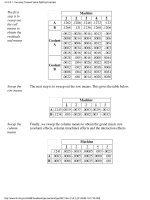
term SD is distinctly larger than the short term SD there are uncorrected error sources at work.

The use of comparison designs, described in chapter 5, facilitates this type of analysis. The
within group variability, σ
w
, is computed for each measurement sequence. Each measurement
sequence includes a check standard that is measured in each calibration. The total standard
deviation, σ
t
is computed for the collection of values for the check standard. The inequality

σ
t
>>σ
w
is taken as evidence of a long term systematic effect, perhaps as yet unidentified. For the
NIST system a very large number of measurements have been made over the years and we have
found, as shown in table 4.1, that except for long blocks there appear to be no uncorrected long
term error sources. The differences for long blocks are probably due to inadequate thermal
preparation or operator effects caused by the difficult nature of the measurement.

Table 4.1

Comparison of Short Term and Long Term Standard Deviations
for Mechanical Gauge Block Comparisons (in nanometers)

Group σ
short term
σ
σlong term


14 1.00 mm to 1.09 mm 5 6
15 1.10 mm to 1.29 mm 5 5
16 1.30 mm to 1.49 mm 5 5
17 1.50 mm to 2.09 mm 5 5
18 2.10 mm to 2.29 mm 5 5
19 2.30 mm to 2.49 mm 5 5
20 2.50 mm to 10 mm 5 5
21 10.5 mm to 20 mm 5 7
22 20.5 mm to 50 mm 6 8

23 60 mm to 100 mm 8 18
24 125 mm 9 19
150 mm 11 38
175 mm 10 22
200 mm 14 37
250 mm 11 48
300 mm 7 64
400 mm 11 58
500 mm 9 56

4.3.5 Error Budgets

An error budget is a systematic method for estimating the limit of error or uncertainty for a
measurement. In this method, one lists all known sources of error which might affect the
measurement result. In the traditional method, a theoretical analysis of error sources is made to
provide estimates of the expected variability term by term. These estimates are then combined to
obtain an estimate of the total expected error bounds.

46

The items in an error budget can be classified according to the way they are most likely to affect
the uncertainty. One category can contain items related to type B uncertainty; another can relate
to σ
w
; and a third category can relate to σ
t
. Since all sources of short term variability also affect
the long term variability, short term effects are sometimes subtracted to give an estimate of the
effects of only the sources of long term variability. This long term or "between group
variability", σ

B
, is simply calculated as (σ
t
-σ
w
). The example in table 4.2 shows a tentative
disposition for the mechanical comparison of gauge blocks.


Table 4.2

Error Source Category

Uncertainty of Master Block systematic

Stylus diameter, pressure and condition long term

Assigned Temperature Coefficients systematic

Temperature difference between blocks long term

Stability of Blocks long term

Environment: vibration, thermal changes,
operator effects short term

Block flatness/ anvil design systematic

Block geometry: effect of flatness
and parallelism on measurement

with gauging point variability short term

Comparator calibration long term

Comparator repeatability short term

Most of the error sources in table 4.2 can be monitored or evaluated by a judicious choice of a
comparison design, to be used over a long enough time so that the perturbations can exert their
full effect on the measurement process. Two exceptions are the uncertainties associated with the
assigned starting values, or restraint values, and the instrument calibration.

Table 4.3 shows error budget items associated with gauge block measurement processes. Listed
(1σ level) uncertainties are typical of the NIST measurement process for blocks under 25 mm
long. The block nominal length, L, is in meters.

47


Table 4.3

Resulting Length
Error Sources
Uncertainty in µm Note

Repeatability 0.004 + 0.12 L (1)

Contact Deformation 0.002 (2)

Value of Master Block 0.012 + 0.08 L

Temperature Difference
Between Blocks 0.17

L (3)

Uncertainty of Expansion
Coefficient 0.20

L (4)


Note 1. Repeatability is determined by analyzing the long term control data. The number
reported is the 1σ
t
value for blocks under 25 mm.

Note 2. For steel and chrome carbide, blocks of the same material are used in the comparator
process and the only error is from the variation in the surface hardness from block to block. The
number quoted is an estimate. For other materials the estimate will be higher.

Note 3. A maximum temperature difference of 0.030 ºC is assumed. Using this as the limit of a
rectangular distribution yields a standard uncertainty of 0.17L.

Note 4. A maximum uncertainty of 1x10
-6
/ºC is assumed in the thermal expansion coefficient,
and a temperature offset of 0.3 ºC is assumed. For steel and chrome carbide blocks we have no
major differential expansion error since blocks of the same material are compared. For other
materials the estimate will be higher.
These errors can be combined in various ways, as discussed in the next section.

4.3.6 Combining Type A and Type B uncertainties

Type A and type B uncertainties are treated as equal, statistically determined and if uncorrelated
are combined in quadrature.

In keeping with current international practice, the coverage factor k is set equal to two (k=2) on
NIST gauge block uncertainty statements.
) (4.2
B
+
A
k =ty UncertainExpanded = U
22
∑∑

48

Combining the uncertainty components in Table 4.3 according to these rules gives a standard
uncertainty (coverage factor k=2)

U = Expanded Uncertainty = 0.026 + 0.32L (4.3)

Generally, secondary laboratories can treat the NIST stated uncertainty as an uncorrelated type B
uncertainty. There are certain practices where the NIST uncertainty should be used with caution.
For example, if a commercial laboratory has a gauge block measured at NIST every year for
nine years, it is good practice for the lab to use the mean of the nine measurements as the length
of the block rather than the last reported measurement. In estimating the uncertainty of the
mean, however, some caution is needed. The nine NIST measurements contain type B
uncertainties that are highly correlated, and therefore cannot be handled in a routine manner.

Since the phase assigned to the NIST master blocks, the penetration, wringing film thickness and
thermal expansion differences between the NIST master and the customer block do not change
over the nine calibrations, the uncertainties due to these factors are correlated. In addition, the
length of the NIST master blocks are taken from a fit to all of its measurement history. Since
most blocks have over 20 years of measurement history, the new master value obtained when a
few new measurements are made every 3 years is highly correlated to the old value since the fit
is heavily weighted by the older data. To take the NIST uncertainty and divide it by 3 (square
root of 9) assumes that all of the uncertainty sources are uncorrelated, which is not true.

Even if the standard deviation from the mean was calculated from the nine NIST calibrations, the
resulting number would not be a complete estimate of the uncertainty since it would not include
the effects of the type B uncertainties mentioned above. The NIST staff should be consulted
before attempting to estimate the uncertainty in averaged NIST data.

4.3.7 Combining Random and Systematic Errors

There is no universally accepted method of combining these two error estimates. The traditional
way to combine random errors is to sum the variances characteristic of each error source. Since
the standard deviation is the square root of the variance, the practice is to sum the standard
deviations in quadrature. For example, if the measurement has two sources of random error
characterized by σ
1
and σ
2
, the total random error is


σ
tot
= [σ

1
2
+ σ
2
2
]
1/2
. (4.4)

This formula reflects the assumption that the various random error sources are independent. If
there are a number of sources of variation and their effects are independent and random, the
probability of all of the effects being large and the same sign is very small. Thus the combined
error will be less than the sum of the maximum error possible from each source.

Traditionally, systematic errors are not random (they are constant for all calibrations) and may
be highly correlated, so nothing can be assumed about their relative sizes or signs. It is logical

49
then to simply add the systematic errors to the total random error:

Total Uncertainty (traditions) = 3σ
tot
+ Systematic Error. (4.5)

The use of 3σ as the total random error is fairly standard in the United States. This corresponds
to the 99.7% confidence level, i.e., we claim that we are 99.7% confident that the answer is
within the 3σ bounds. Many people, particularly in Europe, use the 95% confidence level (2σ)
or the 99% confidence level (2.5σ) rather than the 99.7% level (3σ) used above. This is a small
matter since any time an uncertainty is stated the confidence level should also be stated. The
uncertainty components in Table 4.3 are all systematic except the repeatability, and the

uncertainty calculated according to the traditional method is

Total Uncertainty (traditional) = 3(0.004 + 0.12L) + 0.002 + 0.012 + 0.08L + 0.17L + 0.2L

Total Uncertainty (traditional) = 0.026 + 0.81L


4.4 The NIST Gauge Block Measurement Assurance Program

The NIST gauge block measurement assurance program (MAP) has three parts. The first is a
continual interferometric measurement of the master gauge blocks under process control
supplied by control charts on each individual gauge block. As a measurement history is built up
for each block, the variability can be checked against both the previous history of the block and
the typical behavior of other similar sized blocks. A least squares fit to the historical data for
each block provides estimates of the current length of the block as well as the uncertainty in the
assigned length. When the master blocks are used in the mechanical comparison process for
customer blocks, the interferometric uncertainty is combined in quadrature with the
Intercomparison random error. This combined uncertainty is reported as the uncertainty on the
calibration certificate.

The second part of the MAP is the process control of the mechanical comparisons with customer
blocks. Two master blocks are used in each calibration and the measured difference in length
between the master blocks is recorded for every calibration. Also, the standard deviation derived
from the comparison data is recorded. These two sets of data provide process control parameters
for the comparison process as well as estimates of short and long term process variability.

The last test of the system is a comparison of each customer block length to its history, if one
exists. This comparison had been restricted to the last calibration of each customer set, but since
early 1988 every customer calibration is recorded in a database. Thus, in the future we can
compare the new calibration with all of the previous calibrations. Blocks with large changes are

re-measured, and if the discrepancy repeats the customer is contacted to explore the problem in
more detail. When repeated measurements do not match the history, usually the block has been
damaged, or even replaced by a customer. The history of such a block is then purged from the
database.


50
4.4.1 Establishing Interferometric Master Values

The general practice in the past was to use the last interferometric calibration of a gauge block as
its "best" length. When master blocks are calibrated repeatedly over a period of years the
practice of using a few data points is clearly not the optimum use of the information available. If
the blocks are stable, a suitable average of the history data will produce a mean length with a
much lower uncertainty than the last measurement value.
Reviewing the calibration history since the late fifties indicates a reasonably stable length for
most gauge blocks. More information on stability is given in section 3.5. The general patterns
for NIST master gauge blocks are a very small constant rate of change in length over the time
covered. In order to establish a "predicted value," a line of the form:


L
t
= L
o
+ K
1
(t-t
o
) (4.6)

is fit to the data. In this relation the correction to nominal length (L
t
) at any time (t) is a function
of the correction (L
o
) at an arbitrary time (t
o
), the rate of change (K
1
), and the time interval (t-t
o
).

When the calibration history is short (occasionally blocks are replaced because of wear) there
may not be enough data to make a reliable estimate of the rate of change K
1
. We use a few
simple rules of thumb to handle such cases:

1. If the calibration history spans less than 3 years the rate of change is assumed to
be zero. Few blocks under a few inches have rates of change over 5 nm/year, and
thus no appreciable error will accumulate.

2. A linear least squares fit is made to the history (over 3 years) data. If the
calculated slope of the line does not exceed three times the standard deviation of
the slope, we do not consider the slope to be statistically significant. The data is
then refitted to a line with zero slope.

51

Figure 4.1a. Interferometric history of the 0.1 inch steel master block showing
typical stability of steel gauge blocks.





Figure 4.1b. Interferometric history of the 0.112 inch steel master block showing a predictable
change in length over time.


Figure 4.1a shows the history of the 0.1 inch block, and it is typical of most NIST master blocks.
The block has over 20 years of history and the material is very stable. Figure, 4.1b, shows a block
which has enough history to be considered unstable; it appears to be shrinking. New blocks that

52
show a non-negligible slope are re-measured on a faster cycle and if the slope continues for over 20
measurements and/or 5 years the block is replaced.

The uncertainty of predicted values, shown in figure 4.1 by lines above and below the fitted line, is a
function of the number of points in each collection, the degree of extrapolation beyond the time span
encompassed by these points, and the standard deviation of the fit.

The uncertainty of the predicted value is computed by the relation

(4.7)




where n = the number of points in the collection;

t = time/date of the prediction;

t
a
= average time/date ( the centroid of time span covered by the measurement history, that is
t
a
=Σt
i
/n);

t
i
= time/date associated with each of the n values;

σ = process standard deviation (s.d. about the fitted line);

σ
t
= s.d. of predicted value at time t.

In figure 4.2 the standard deviations of our steel inch master blocks are shown as a function of
nominal lengths. The graph shows that there are two types of contributions to the uncertainty, one
constant and the other length dependent.









)
t
-
t
(
)
t
-(t
+
n
1
3 = 3
2
ai
2
a
t
∑

σ
σ

53


Figure 4.2. Plot of standard deviations of interferometric length history of NIST
master steel gauge blocks versus nominal lengths.

The contributions that are not length dependent are primarily variations in the wringing film
thickness and random errors in reading the fringe fractions. The major length dependent component
are the refractive index and thermal expansion compensation errors.

The interferometric values assigned to each block from this analysis form the basis of the NIST
master gauge block calibration procedure. For each size gauge block commonly in use up to 100
mm (4 in.), we have two master blocks, one steel and one chrome carbide. Blocks in the long series,
125 mm (5 in.) to 500 mm (20 in.) are all made of steel, so there are two steel masters for each size.
Lengths of customer blocks are then determined by mechanical comparison with these masters in
specially designed sequences.

4.4.2 The Comparison Process

There are currently three comparison schemes used for gauge block measurements. The main
calibration scheme uses four gauge blocks, two NIST blocks and two customer blocks, measured six
times each in an order designed to eliminate the effects of linear drift in the measurement system.
For gauge blocks longer than 100mm (4 in.) there are two different schemes used. For most of these
long blocks a procedure using two NIST blocks and two customer blocks measured four times each
in a drift eliminating design is used. Rectangular blocks over 250 mm are very difficult to
manipulate in the comparators, and a reduced scheme of two NIST masters and one customer block
is used.

Comparators and associated measurement techniques are described in chapter 5. In this chapter,
only the measurement assurance aspects of processes are discussed. The MAP for mechanical
comparisons consists of a measurement scheme, extraction of relevant process control parameters,

54
process controls, and continuing analysis of process performance to determine process uncertainty.

4.4.2.1 Measurement Schemes - Drift Eliminating Designs

Gauge block comparison schemes are designed with a number of characteristics in mind. Unless
there are extenuating circumstances, each scheme should be drift eliminating, provide one or more
control measurements, and include enough repeated comparisons to provide valid statistics. Each of
these characteristics is discussed briefly in this section. The only scheme used at NIST that does not
meet these specifications is for long rectangular blocks, where the difficulty in handling the blocks
makes multiple measurements impractical.

In any length measurement both the gauge being measured and the measuring instrument may
change size during the measurement. Usually this is due to thermal interactions with the room or
operator, although with some laser based devices changes in the atmospheric pressure will cause
apparent length changes. The instrumental drift can be obtained from any comparison scheme with
more measurements than the number of unknown lengths plus one for drift, since the drift rate can
be included as a parameter in the model fit. For example, the NIST comparisons include six
measurements each of four blocks for a total of 24 measurements. Since there are only three
unknown block lengths and the drift, least squares techniques can be used to obtain the best estimate
of the lengths and drift. It has been customary at NIST to analyze the measurements in pairs,
recording the difference between the first two measurements, the difference between the next two
measurements, and so on. Since some information is not used, the comparison scheme must meet
specific criteria to avoid increasing the uncertainty of the calibration. These designs are called drift
eliminating designs.

Besides eliminating the effects of linear instrumental drift during the measurements, drift eliminating
designs allow the linear drift itself to be measured. This measured drift can be used as a process
control parameter. For small drift rates an assumption of linear drift will certainly be adequate. For
high drift rates and/or long measurement times the assumption of linear drift may not be true. The
length of time for a measurement could be used as a control parameter, but we have found it easier to
restrict the measurements in a calibration to a small number which reduces the interval and makes
recording the time unnecessary.

As an example of drift eliminating designs, suppose we wish to compare two gauge blocks, A and B.
At least two measurements for each block are needed to verify repeatability. There are two possible
measurement schemes: [ A B A B ] and [ A B B A ]. Suppose the measurements are made equally
spaced in time and the instrument is drifting by some ∆ during each interval. The measurements
made are:




55
Measurement Scheme ABAB Scheme ABBA

m
1
A A (4.8)
m
2
B + ∆ B + ∆
m
3
A + 2∆ B + 2∆

m
4
B + 3∆ A + 3∆

If we group the measurements into difference measurements:

Scheme ABAB Scheme ABBA

y
1
= m
1
- m
2
= A - (B + ∆) A - (B + ∆) (4.9a)
y
2
= m
3
- m
4
= (A+2∆)-(B+3∆) (B + 2∆)-(A+3∆) (4.9b)


Solving for B in terms of A:

B = A - (y
1
+y
2

)/2 - ∆ A - (y
1
-y
2
)/2 (4.10)

In the first case there is no way to find B in terms of A without knowing ∆, and in the second case
the drift terms cancel out. In reality, the drift terms will cancel only if the four measurements are
done quickly in a uniformly timed sequence so that the drift is most likely to be linear.

A general method for making drift eliminating designs and using the least squares method to analyze
the data is given in appendix A.

The current scheme for most gauge block comparisons uses two NIST blocks, one as a master block
(S) and one as a control (C), in the drift eliminating design shown below. Two blocks, one from
each of two customers, are used as the unknowns X and Y. The 12 measured differences, y
i
, are
given below:

y
1
= S - C
y
2
= Y - S
y
3
= X - Y
y

4
= C - S
y
5
= C - X
y
6
= Y - C (4.11)
y
7
= S - X
y
8
= C - Y
y
9
= S - Y
y
10
= X - C
y
11
= X - S
y
12
= Y - X

56

(4.12)



The calibration software allows the data to be analyzed using either the S block or the C block as the
known length (restraint) for the comparison. This permits customer blocks of different materials to
be calibrated at the same time. If one customer block is steel and the other carbide, the steel master
can be used as the restraint for the steel unknown, and the carbide master can be used for the carbide
unknown. The length difference (S-C) is used as a control. It is independent of which master block
is the restraint.

There is a complete discussion of our calibration schemes and their analysis in appendix A. Here we
will only examine the solution equations:



S = L (reference length) (4.13a)

C = (1/8) (-2y
1
+ y
2
+ 2y
4
+ y
5
- y
6
- y
7

+ y
8
- y
9
- y
10
+ y
11)
+ L (4.13b)

X = (1/8) (-y
1
+ y
2
+ y
3
+ y
4
- y
5
- 2y
7
- y
9
+ y
10
+ 2y
11
- y
12

) + L (4.13c)

Y = (1/8) (-y
1
+ 2y
2
- y
3
+ y
4
+ y
6
- y
7
- y
8
- 2y
9
+ y
11
+ y
12
) + L (4.13d)

∆ = (-1/12)(y
1
+y
2
+y
3

+y
4
+y
5
+y
6
+y
7
+y
8
+y
9
+y
10
+y
11
+y
12
) (4.13e)


The standard deviation is calculated from the original comparison data. The value of each
comparison, <y
i
>, is calculated from the best fit parameters and subtracted from the actual data, y
i
.
The square root of the sum of these differences squared divided by the square root of the degrees of
freedom is taken as the (short term or within) standard deviation of the calibration:

For example,


∆y
12
= (C - B) - y
12
(4.14a)

= (1/8) (y
2
-2y
3
+ y
5
+y
6
+ y
7
- y
8
- y
9
- y
10
- y
11
) - y
12

(4.14b)


These deviations are used to calculate the variance.
/8
)
Y
( =
2
i
12
0i=
w
2
∆
σ
∑