Financial Toolbox For Use with MATLAB Computation Visualization Programming phần 2 pptx
Bạn đang xem bản rút gọn của tài liệu. Xem và tải ngay bản đầy đủ của tài liệu tại đây (261.46 KB, 40 trang )
1 Tutorial
1-28
The default basis is actual days if none is specified. The toolbox basi s choices
are:
Thus you can compute the difference between two dates in four different ways.
The first way (
basis = 0) simply returns the difference in actual days between
two dates. The second (
basis = 1) returns the difference, but adjusted to a
360-day year in which all months have 30 days. The third and fourth methods
return a difference in dates as a fraction of either a 360- or 365-day year,
respectively.
Determining Dates
The toolbox provides many functions for determining specific dates, including
functions which account for holidays and other non-trading days.
For example, you schedule an accounting procedure for the last Friday of every
month. The
lweekdate function returns those dates for 1998; the 6 sp ecifies
Friday:
fridates = lweekdate(6, 1998, 1:12);
fridays = datestr(fridates)
fridays =
30-Jan-1998
27-Feb-1998
27-Mar-1998
24-Apr-1998
29-May-1998
26-Jun-1998
31-Jul-1998
28-Aug-1998
25-Sep-1998
30-Oct-1998
27-Nov-1998
25-Dec-1998
basis = 0
Actual days (default)
basis = 1
360-day year (assumes all months are 30 days)
basis = 2
Actual days/360
basis = 3
Actual days/365
Understanding the Financial Toolbox
1-29
Or your company cl os es o n Ma rti n Luther K in g Jr. Day, which is t he third
Monday in January. The
nweekdate functi on determines those dat es for 19 9 8
through 2001:
mlkdates = nweekdate(3, 2, 1998:2001, 1);
mlkdays = datestr(mlkdates)
mlkdays =
19-Jan-1998
18-Jan-1999
17-Jan-2000
15-Jan-2001
Accounting for holidays and other non-trading days is important when
examining financial dates. The toolbox provides the
holidays function, which
contains holidays and special non-trading days for the New York Stock
Exchange between 1950 and 2030, inclusive. You can edit the
holidays.m file
to customize it with your own holidays and non-trading days. In this example,
use it to determine the standard holidays in the last half of 1998:
lhhdates = holidays('1-Jul-1998', '31-Dec-1998');
lhhdays = datestr(lhhdates)
lhhdays =
03-Jul-1998
07-Sep-1998
26-Nov-1998
25-Dec-1998
Now use the toolbox busdate function to determine the next business day after
these holidays:
lhnextdates = busdate(lhhdates);
lhnextdays = datestr(lhnextdates)
lhnextdays =
06-Jul-1998
08-Sep-1998
27-Nov-1998
28-Dec-1998
The toolbox also provides the cfdates function to determine cash-flow dates for
securities with periodic payments. This function accounts for the coupons per
1 Tutorial
1-30
year, the day-count basis, and the end-of-month rule. For example, to
determine the cash-flow dates for a security that pays four coupons per year on
the last day of the month, on an actual/365 day-count basis, just enter the
settlement date, the maturity date, and the parameters:
paydates = cfdates('14-Mar-1997', '30-Nov-1998', 4, 3, 1);
paydays = datestr(paydates)
paydays =
31-May-1997
31-Aug-1997
30-Nov-1997
28-Feb-1998
31-May-1998
31-Aug-1998
30-Nov-1998
Formatting Currency and Charting Financial Data
The Financial Toolbox provides several functions to format currency and chart
financial data.
Currency Formats
The currency formatting functions are:
These examples show their use
dec = frac2cur('12.1', 8)
returns dec = 12.125, which is the decimal equivalent of 12-1/8. The second
input variable is the denominator of the fraction.
str = cur2str(−8264, 2)
returns the string ($8264.00). For this toolbox function, the output format is
a numerical format with dollar sign prefix, two decimal places, and negative
numbers in parentheses; e.g.,
($123.45) and $6789.01.Thestandard
cur2frac
Converts decimal currency values to fractional values
cur2str
Converts a value to Financial Toolbox bank format
frac2cur
Converts fractio nal currency values to decimal values
Understanding the Financial Toolbox
1-31
MATLAB bank format uses two decimal places, no dollar sign, and a minus
sign for neg ative numbers ; e.g.,
−123.45 and 6789.01.
Financial Charts
The toolbox financial charting functions
plot financial data and produce presentation-quality figures quickly and easily.
They work with standard MATLAB functions that draw axes, control
appearance, and add labels and titles.
Here are two plotting examples: a high-low-close chart of sample IBM stock
price data, and a Bollinger band chart of the same data. These examples load
data from an external file (
ibm.dat), then call the functions using subsets of the
data.
ibm is an R-by-6 matrix where each row R is a trading day’s data and
where columns 2, 3, and 4 contain the high, low, and closing prices,
respectively.
Note: The data in ibm.dat is fictional and for illustrative use only.
High-Low-Close Chart Example. First load the data and set up matrix dimensions.
load and size are standard MATLAB functions.
load ibm.dat;
[ro, co] = size(ibm);
Open a figure window for the chart. Use the Financial Toolbox highlow
function to plot high, low, and close prices for the last 50 trading days in the
data file.
figure;
highlow(ibm(ro−50:ro,2),ibm(ro−50:ro,3),ibm(ro−50:ro,4),[],'b');
bolling
Bollinger band chart
candle
Candlestick chart
pointfig
Point and figure chart
highlow
High, low, open, close chart
movavg
Leading and lagging moving averages chart
1 Tutorial
1-32
Add labels and title, and set axes with standard MATLAB functions. Use the
Financial Toolbox
dateaxis function to provide dates for the x-axis ticks.
xlabel('');
ylabel('Price ($)');
title('International Business Machines, 941231 - 950219');
axis([0 50 −inf inf]);
dateaxis('x',6)
MATLAB produces a figure similar to this. The plotted data and axes you see
may differ. On a color monitor, the high-low-close bars are blue.
Bollinger Chart Example. Next the Financial Toolbox bolling function produces a
Bollinger band chart using all the closing prices in the same IBM stock price
matrix. A Bollinger band chart plots actual data along with three other bands
of data. The upper band is two standard deviations above a moving average;
the lower band is two standard deviations below that moving average; and the
12/31 01/10 01/20 01/30 02/09 02/19
86
88
90
92
94
96
98
Price ($)
International Business Machines, 941231 − 950219
Understanding the Financial Toolbox
1-33
middle band is the moving average itself. This example uses a 15-day moving
average.
Assuming the previous IBM data is still loaded, simply execute the Financial
Toolbox function.
bolling(ibm(:,4), 15, 0);
Specify the axes, labels, and titles. Again, use dateaxis to add the x-axis dates.
axis([0 ro min(ibm(:,4)) max(ibm(:,4))]);
ylabel('Price ($)');
title(['International Business Machines']);
dateaxis('x', 6)
MATLAB does the rest. On a color monitor, the red lines are the upper and
lower bands, the green line is the 15-day simple moving average, and the blue
line charts the actual price data. In this reproduction, the outer lines are the
upper and lower bands, the middle smo oth line is the moving average, and the
middle jagged line is the actual price data. Again, the plotted data and axes
you see may differ from this reproduction.
1 Tutorial
1-34
For help using MATLAB plotting functions, see the “Graphics” section of
Getting Started with MATLAB. See Using MATLAB Graphics f or details on
the
axis, title, xlabel,andylabel functions.
Analyzing and Computing Cash Flows
The Financial Toolbox cash-flow functions compute interest rates, payments,
present and future values, annuities, rates of return, and depreciation streams.
Some examples in this section use this income stream: an initial investment of
$20,000 followed by three annual return payments, a second investment of
$5,000, then four more returns. Investments are negative cash flows, return
payments are positive cash flows.
stream = [−20000, 2000, 2500, 3500, −5000, 6500,
9500, 9500, 9500];
12/31 02/19 04/09 05/29 07/18 09/06 10/26 12/15 02/03
45
50
55
60
65
70
75
80
85
90
95
Price ($)
International Business Machines
Understanding the Financial Toolbox
1-35
Interest Rates / Rates of Return
Several functions calculate interest rates involved with cash flows. To compute
the internal rate of return of the cash stream, simply execute the toolbox
function
irr
ror = irr(stream)
whichgivesarateofreturnof11.72%.
Note that the internal rate of return of a cash flow may not have a unique
value. Every time the sign changes in a cash flow, the equation defining
irr
can give up to two additional answers. An irr computation requires solving a
polynomial equation, and the number of real roots of such an equation can
depend on the number of sign changes in the coefficients. The equa tion for
internal rate of return is
where Investment is a (negative ) in itia l cas h o utla y a t tim e 0, cf
n
is the cash
flow in the nth period, and n is the number of periods. Basically,
irr finds the
rate r such that the net pre sent value of the cash flo w equals the initial
investm ent. If all of the cf
n
s are positive there is only one solution. Every time
there is a change of sign between coefficients, up to two additional real roots
are possible. There is usually only one answer that makes sense, but it is
possible t o get returns of b oth 5% and 11% (for example ) from on e income
stream.
Another toolbox rate function,
effrr, calculates the effect ive rate of return
given an annual interest rate (also known as nominal rate or annual
percentage rate, APR) and number of compounding periods per year. To ask
for the effective rate of a 9% APR compounded monthly, simply enter:
rate = effrr(0.09, 12)
The answer is 9.38%.
A companion function
nomrr computes the nominal rate of return given the
effective annual rate and the number of compounding periods.
cf
1
1 r+()
cf
2
1 r+()
2
…
cf
n
1 r+()
n
Investment++++ 0=
1 Tutorial
1-36
Present / Future Values
The toolbox includes functions to compute the present or future value of cash
flows at regular or irregular time intervals with equal or unequal payments:
fvfix, fvvar, pvfix,andpvvar.The-fix functions assume equal cash flows
at regular intervals, while the
-var functions allow irregular cash flows at
irregular periods.
Now compute the net present value of the sample income stream for which you
computed the i nte rnal rat e of r eturn. This exercise also serves as a check on
that calculation because the net present value of a cash stream at its internal
rate of return should be zero. Enter
npv = pvvar(stream, ror)
which returns 2.6830e-011, or 0.000000000026830— very close to zero. The
answer usually is not exactly zero due to rounding errors and the
computational precision of the computer.
Note: Some other toolbox functions behave similarly. T he functions that
compute a bond’s yield, for example, often must solve a nonlinear equation. If
you then use that yield to compute the net present value of the bond’s income
stream, it usually doe s not exactly equal the purchase price — but the
difference is negligible for practical applications.
Sensitivity
The Financial Toolbox can also compute the Macaulay duration for a cash flow
where all values in the stream are not necessarily the same. The Macaulay
duration measures how long, on average, the owner waits before receiving a
payment.
cfdur computes the Macaulay duration and modified duration
(volatility) of a cash stream.
Returning to the sample cash flow and using a discount rate of 6%, this
example
rate = 0.06;
[duration, moddur] = cfdur(stream, rate)
gives a duration of 23.49 periods and a modified duration (volatility) of 22.16
periods. The length of these periods is the same as the length of the periods in
Understanding the Financial Toolbox
1-37
the cash flow. Note that using the computed internal rate of return as the
discount rate is not appropriate, since a cash flow wit h net present value of 0
has infinite duration.
Depreciation
The toolbox includes functions to compute standard depreciation schedules:
straight line, general declining-balance, fixed declining-balance, and sum of
years’ digits. Functi ons also compute a co mpl ete amortizat io n schedule for an
asset, and return the remaining depreciable value after a depreciation
schedule ha s bee n app lie d.
This example depreciates an automobile worth $15,000 over five years with a
salvage value of $1,500. It computes the general declining balance using two
different depreciati on ra te s: 50% ( or 1 .5), a nd 1 00% (or 2.0, also known a s
double declining balance). Enter
decline1 = depgendb(15000, 1500, 5, 1.5)
decline2 = depgendb(15000, 1500, 5, 2.0)
which returns
decline1 =
4500.00 3150.00 2205.00 1543.50 2101.50
decline2 =
6000.00 3600.00 2160.00 1296.00 444.00
These functions return the actual depreciation amount for the first four years
and the remaining depreciable value as the entry for the fifth year.
Annuities
Several toolbox functions deal with annuities. This first example shows how to
compute the interest rate associated with a series of loan payments when only
the payment amounts and principal are known. For a loan whose original
value was $5000.00 and which was paid back monthly over four years at
$130.00/month:
rate = annurate(4*12, 130, 5000, 0, 0)
The function returns a rate of 0.0094 monthly, or approximately 11.28%
annually.
1 Tutorial
1-38
The next example uses a present-value function to show how to compute the
initial principal when the payment and rate are known. For a loan paid at
$300.00/month over four years at 11% annual interest:
principal = pvfix(0.11/12, 4*12, 300, 0, 0)
The function returns the original principal value of $11,607.43.
The final example computes an amortization schedule for a loan or annuity.
The original value was $5000.00 and was paid back over 12 months at an
annual rate of 9%.
[prpmt, intpmt, balance, payment] =
amortize(0.09/12, 12, 5000, 0, 0);
This function returns vectors containing the amount of principal paid,
prpmt = [402.76 405.78 408.82 411.89 414.97 418.09
421.22 424.38 427.56 430.77 434.00 437.26]
the amount of interest paid,
intpmt = [34.50 31.48 28.44 25.37 22.28 19.17
16.03 12.88 9.69 6.49 3.26 0.00]
the remaining balance for each period of the loan,
balance = [4600.24 4197.49 3791.71 3382.89 2971.01
2556.03 2137.94 1716.72 1292.34 864.77
434.00 0.00]
and a scalar for the monthly payment.
payment = 437.26
Pricing and Computing Yields for Fixed-Income
Securities
The Financial Toolbox includes many functions t o compute accrued interest,
determine prices and yields, cal culate convexity and duration of fixed-income
securities, and generate and analyze term structure of interest rates.
Understanding the Financial Toolbox
1-39
Terminology
Since terminology varies among texts on this subject, here are some basic
definitions that apply t o thes e Financial Toolbox fun ctions. You can also find
these and other defini ti ons i n the Glossary.
The
settlement date of a bond i s the date when money first cha n ges hands; i.e.,
when a buyer pays for a bond. It need not coincide with the issue date. The
issue date is the date a bond is first offered for sale. That date usually
deter mine s whe n interest payments, known as
coupons, are made. The first
and last
coupon dates are the dates w hen the first and last coupons a re paid.
Typically a bond pays coupons annually or semi-annually.
Fixed-income securities can be purchased on dates that do not coincide with
coupon or payment dates. The length of the first and last periods may differ
from t he regular coupon period, a nd thus the bond owner is not entitled to the
full value of t he co upon fo r that p eriod. Instead, t he coup on is pro -rated
according t o how long the b o nd is h el d d uring t h at p e r io d. The toolb ox incl udes
price and yield functions tha t handle o dd first period , odd las t period, and odd
first and last perio ds.
The
maturity date of a b ond is the date when the issuer returns t he final face
value, also known as the
redemption value or par value,tothebuyer.
Typically the
purchase price, t he price actually paid for a bond, is not the
same as the redemption value. The
yiel d of a bond is d et ermined by the ratio
of redemption value to purchas e price over the life of the bond. It is the nominal
annual interest rate that gives a
future value o f the purchase p rice equal t o
the redemption value o f t he bo nd. T he cou pon payments d etermine part of th at
yield.
In the Ref erence chapte r, these fixe d-income f unctions use standard
abbreviations for variables.
Abbreviation Refers To
p
Price
ai
Accrued interest
sd
Settlement date
md
Maturity date
1 Tutorial
1-40
Pricing Functions
This example shows how easily you can compute the p rice o f a bond with an odd
first period. It uses the standard abbreviations to set up the input variables.
sd = '11/11/1992';
md = '03/01/2005';
id = '10/15/1992';
fd = '03/01/1993';
cpn = 0.0785;
yld = 0.0625;
per = 2;
basis = 0;
eom = 1;
Simply executing the function bndprice
[pr, ai] = bndprice(yld, cpn, sd, md, per, basis, eom, id, fd)
returns a price, pr = 113.60 and accrued interest, ai = 0.59.
Similar functions compute prices with regular payments, payment at maturity,
and odd first and last periods, as well as prices of Treasury bills and discounted
securities such as zero-coupon bonds.
id
Issue date
fd
First coupon date
lcd
Last coupon date
rv
Redemption value
cpn
Coupon rate
yld
Bond yield
per
Coupons per year
basis
Day-count basis
eom
Endofmonthrule
Abbreviation Refers To
Understanding the Financial Toolbox
1-41
Yield Functions
To illustr ate toolbox yield funct ions, this exampl e computes the yield of a bond
that has odd first and last periods and s et tlement in the first period. It uses
descriptive variable names rather than the standard abbreviations. First set
up variables for settlement date, maturity date, issue date, first coupon date
(
fcoup), and a last coupon date (lcoup).
settledate = '12-Jan-1994';
maturedate = '1-Oct-1995';
issuedate = '1-Jan-1994';
fcoup = '15-Jan-1994';
lcoup = '15-Apr-1994';
Now for a redemption value of $100.00, supply a purchase price of $95.70,
coupon rate of 4%, paying coupons four times a year, and assume a 36 0-day
year of equal 30-day months (
basis = 1). To find the answer the function solves
a nonlinear equation using at most 50 iterations.
purch = 95.7;
coupr = 0.04;
freq = 4;
basis = 1;
eom = 1;
Call the fun ctio n
bndyield(purch, coupr, settledate, maturedate, freq, basis,
eom, issuedate, fcoup, lcoup)
which returns the yield of 6.73%.
You can also use vectors for each of these arguments but be careful that each
vector has the same number of arguments. You receive a vector of yields in
return. Using vectors computes yields for several securities at once.
Toolbox functions also co mpute yields of Treasury bills and fixed-income
securities with payments at regular times or at maturity. For example, using
the previous dates and redemption value, a price of $95.00 and a 6% coupon
rate, this function
price = 95.0;
cpn = 0.06;
yldmat(settledate, maturedate, issuedate, redeem, price, cpn)
1 Tutorial
1-42
calculates a 13.62% yield for a security whose interest is paid at maturity.
Fixed-Income Sensitivities
The toolbox includes functions to perform sensitivity analysis such as convexity
and the Macaulay and modified durations for fixed-income securities. The
Macaulay duration of an income stream, such as a coupon bond, measures how
long, on average, the owner waits before receiving a payment. It is the
weighted average of the times payments are made, with the weights at time T
equal to the present value of the money received at time T. The modified
duration is the Macaulay duration discounted by the per-period interest rate;
i.e., divided by (1+rate/frequency). Modified duration is also known as
volatility.
To illustrate, this example computes the Macaulay and modified durations for
a bond with settlement and maturity dates as above, a redemption or par value
of $100.00, a 5% coupon rate, a 4.5% yield, semi-annual coupons, and date basis
=0(actualdays).
redeem = 100;
cpn = 0.05;
freq = 2;
yld = 0.045;
[Mac, Mod] = bonddur(settledate, maturedate, redeem, cpn,
yld, freq, 0);
The durations are (in years):
[Mac, Mod] = [0.7049 0.6894]
Term Structure of Interest Rates
The toolbox contains several functions to derive and analyze interest rate
curves, including data conversion and extrapolation, bootstrapping, and
interest-rate curve conversion functions.
One of the first problems in analyzing the term structure of interest rates is
dealing with market data reported in different formats. Treasury bills, for
example, are quoted with bid and asked bank-discount rates. Treasury notes
and bonds, on the other hand, are quoted with bid and asked prices based on
$100 face value. To examine the full spectrum of Treasury secur ities, analysts
must convert data to a single format. Toolbox functions ease this conversion.
Understanding the Financial Toolbox
1-43
In this brief example, we use only one security each; analysts often use 30, 100,
or more of each.
First, capture Treasury bill qu otes in th eir reported format
Maturity Days Bid Ask AskYield
tbill = [datenum('12/26/1997') 53 0.0503 0.0499 0.0510];
then capture Treasury bond quotes in their reported format
Coupon Maturity Bid Ask AskYield
tbond = [0.08875 datenum(1998,11,4) 103+4/32 103+6/32 0.0564];
and note that these quotes a re based on a November 3, 1997 settlement date.
settle = datenum('3-Nov-1997');
Next use the toolbox tbl2bond function to convert the Treasury bill data to
Treasury bond format:
tbtbond = tbl2bond(tbill)
tbtbond =
0 729750 99.259 99.265 0.052091
(The second element o f tbtbond is the s erial date number for December 26,
1997.)
Now combine short-term (Treasury bill) with long-term (Treasury bond) data
to set up the ov erall term structure.
tbondsall = [tbtbond; tbond]
tbondsall =
0 729750 99.259 99.265 0.052091
0.08875 730063 103.125 103.1875 0.0564
The toolbox provides a second data-preparation function, tr2bonds,toconvert
the bond data into a form ready for the bootstrapping functions.
tr2bonds
generates a matrix of bond information sorted by maturity date, plus vectors of
prices and yields.
[bonds, prices, yields] = tr2bonds(tbondsall);
With this market data, we are now ready to use one of the toolbox
bootstrapping functions to derive an implied zero curve. Bootstrapping is a
1 Tutorial
1-44
process whereby you begin with known data points and solve for unknown data
points using an underlying arbitrage theory. Every coupon bond can be valued
as a package of zero-coupon bonds which mimic its cash flow and risk
characteristics. By mapping yields-to-maturity for each theoretical
zero-coupon bond, to the dates spanning the investment horizon, we can create
a theoretical zero-rate curve. The toolbox provides two bootstrapping functions:
zbtprice derives a zero curve from bond data and prices,andzbtyield derives
a zero curve from bond data and yields.Weuse
zbtprice
[zerorates, curvedates] = zbtprice(bonds, prices, settle)
zerorates =
0.051107
0.054501
curvedates =
729750
730063
where curvedates gives the investment horizon.
datestr(curvedates)
ans =
26-Dec-1997
04-Nov-1998
Additional toolbox functions construct discount, forward, and par yield curves
from the zero curve, and vice-versa:
[discrates, curvedates] = zero2disc(zerorates, curvedates, settle);
[fwdrates, curvedates] = zero2fwd(zerorates, curvedates, settle);
[pyldrates, curvedates] = zero2pyld(zerorates, curvedates, settle);
Pricing and Analyzing Equity Derivatives
These toolbox functions compute prices, sensitivities, and profits for portfolios
of options or other equity derivatives. They use the Black-Scholes model for
European options and the binomial model for American options. Such
measures are useful for managing portfolios and for executing collars, hedges,
and straddles.
Understanding the Financial Toolbox
1-45
Sensitivity Measures
There are six basic sensitivity measures associated with option pricing: delta,
gamma, lambda, rho, theta, and vega — the “greeks.” The toolbox provides
functions for calculating each sensitivity and for implied volatility.
Delta
Deltaofaderivativesecurityistherateofchangeofitspricerelativetothe
price of the underlying asset. It is the first de rivative of the curve that relates
thepriceofthederivativetothepriceoftheunderlyingsecurity. Whendelta
is large, the price of the derivative is sensitive to small changes in the price of
the underlying security.
Gamma
Gamma of a derivative security is the rate of change of delta relative to the
price of the underlying asset; i.e., the second derivative of the option price
relative to the security price. When gamma is small, the c hange d elta is small.
This sensitivity measure is important for deciding how much to adjust a hedge
position.
Lambda
Lambda, also known as the elasticity of an option, represents the percentage
change in the price of an option relative to a 1% change in th e price of the
underlying security.
Rho
Rho is the rate of change in option price relative to the underlying security’s
risk-free interest rate.
Theta
Theta is the rate of change in the price of a derivative security relative to time.
Theta is usually very small or negative since the value of an option tends to
drop as it approaches maturity.
Vega
Vegaistherateofchangeinthepriceofaderivativesecurityrelativetothe
volatility of the underlying security. When vega is large the security is
sensitive to small changes in volatility. For example, options traders often
1 Tutorial
1-46
must decide whether to buy an option to hedge against vega or gamma. The
hedge selected usually depends upon how frequently one rebalances a hedge
position and also upon the variance of the price of the underlying asset (the
volatility). If the variance is changing rapidly, balancing against vega is
usually preferable.
Implied Volatility
The implied volatility of an o ption is the v ariance t hat makes a c all option price
equal to the market price. It is used to determine a market estimate for the
future volatility of a stock and provides the input volatility (when needed) to
the other Black-Scholes functions.
Analysis Models
Toolbox functions for analyzing equity derivatives use the Black-Scholes model
for European options and the binomial model for American options. The
Black-Scholes model makes several assumptions about the underlying
securities and their behavior. The binomial model, on the other hand, makes
far fewer assumptions about t he processes underlying an option. For further
explanation, please see the book by John Hull liste d in the Bibliography.
Black-Scholes Model
Using the Black-Scholes model entails several assumptions:
• The option price follows an Ito process.
• The o pt io n can be e x ercis e d only on its expirati on d at e.
• Short sel lin g is permi tte d .
• There are no transaction costs.
• All se curities are d ivisi ble and pay no dividends .
• There is no riskl es s arbitrage.
• Trading is a continuous process.
• The ris k- free interest rat e is constant and remains the sam e for all
maturities.
If any of these assumptions is untrue, Black-Scholes may not be an appropriate
model.
Understanding the Financial Toolbox
1-47
To il lu st ra te toolbox Bla ck -S chol es functio ns, this exampl e c omputes the ca ll
and put prices of a European option and its delta, gamma, lambda, and implied
volatility. The asset price is $100.00, the exercise price is $95.00, the risk-free
interest rate is 10%, the time to maturity is 0.25 years, the volatility is 0.50,
and the dividend rate is 0. Simply executing the toolbox functions:
[optcall, optput] = blsprice(100, 95, 0.10, 0.25, 0.50, 0);
[callval, putval] = blsdelta(100, 95, 0.10, 0.25, 0.50, 0);
gammaval = blsgamma(100, 95, 0.10, 0.25, 0.50, 0);
vegaval = blsvega(100, 95, 0.10, 0.25, 0.50, 0);
[lamcall, lamput] = blslambda(100, 95, 0.10, 0.25, 0.50, 0);
yields
• The option call price
optcall = $13.70
• The option put price
optput = $6.35
• delta for a call
callval = 0.6665 and delta for a put putval = −0.3335
• gamma
gammaval = 0.0145
• vega
vegaval = 18.1843
• lambda for a call
lamcall =4.8664andlambdaforaputlamput = –5.2528
Now as a computation check, find the implied volatility of the option using the
call option price from
blsprice.
volatility = blsimpv(100, 95, 0.10, 0.25, optcall);
The function returns an implied volatility of 0.500, the original blsprice input.
Binomial Model
The binomial model for pricing options or other equity derivatives assumes
that the probability ove r time o f ea c h possible p rice fo ll ows a binomial
distribution. The basic assumption is that prices can move to only two values,
one up and one down, over any short time period. Plotting the two values, and
then the subsequent two values each, and then the subsequent two values
each, and so on over time, is known as “b uild ing a binomial tree.” This mo del
applies to American options, which can be exercised any time up to and
including their expiration date .
1 Tutorial
1-48
This example prices an American call option using a binomial model. Again,
the asset price is $100.00, the exercise price is $95.00, the risk-free interest
rate is 10%, and the time to maturity is 0.25 years. It computes the tree in
increments of 0.05 years, so there are 0.25/0.05 = 5 periods in the example. The
volatility is 0.50, this is a call (
flag = 1), the dividend rate is 0, and it pays a
dividend of $5.00 after three periods (an ex-dividend date). Executing the
toolbox function
[optionpr, optionval] = binprice(100, 95, 0.10, 0.25, 0.05,
0.50, 1, 0, 5.0, 3);
yields the option prices optionpr =
100.00 111.27 123.87 137.96 148.69 166.28
0 89.97 100.05 111.32 118.90 132.96
0 0 81.00 90.02 95.07 106.32
0 0 0 72.98 76.02 85.02
000060.79 67.98
0000054.36
and the option values optionval =
12.10 19.17 29.35 42.96 54.17 71.28
0 5.31 9.41 16.32 24.37 37.96
0 0 1.35 2.74 5.57 11.32
000000
000000
000000
The output from the binomial function is a binary tree. Read the option prices
matrix this way: column 1 shows the price for period 0, column 2 shows the up
and down prices for period 1, column 3 shows the up-up, up-down, and
down-down prices for period 2, etc. Ignore the zeros. The option value matrix
gives the associated option value for each node in the price tree. Ignore the
zeros that correspond to a zero in the p rice t ree.
Analyzing Portfolios
Portfolio manag e r s conce nt rate their effort s on achi eving the be s t po ss ible
trade-off between risk and return. For portfolios constructed from a fixed set of
assets, the risk/re turn profile varie s wit h the portfolio compos it io n. Po rtf o lio s
that maximize the return, given the risk, or, conversely, minimi ze the risk for
Understanding the Financial Toolbox
1-49
the given return, are called optimal. Optimal portfolios define a line in the risk/
return plane called the effici ent fr ontier.
A portfolio may also have to meet additional requirements to be considered.
Different investors have different levels of risk tolerance. Selecting the
adequate portfolio for a particular investor is a difficult process. The portfolio
manager can hed ge the risk related to a particular p ortfolio along the efficient
frontier with partial investment in risk-free assets. The definition of the capital
allocation line, and finding where the final portfolio falls on this line, if at all,
is a function of:
• T he r isk/return profile of e ach ass et
• The risk- fr ee r a te
• T he borrowing rate
• T he d egree of ris k avers ion characterizing an i nvestor
The Financial Toolbox includes a set of functions designed to solve the problem
of finding the portfolio that best meets the requirements of investors, while
considering all parameters.
Portfolio Optimization Functions
The portfolio optimization functions assist portfolio managers in constructing
portfolios that optimize risk and return.
Capital Allocation
portalloc
Computes the optimal risky portfolio on the efficient frontier,
based on the risk-free rate, the borrowing rate, and the
investor's degree of risk aversion. Also generates the capital
allocation line, which provides the optimal allocation of funds
between the risky portfolio and the risk-free ass et.
1 Tutorial
1-50
Efficient Frontier Computation
frontcon
Computes port fol ios along the efficient frontier f o r a given
group of asset s. The computati on is ba sed on sets of
constraints representing the maximum and minimum weights
for each asset, and the maximum and minimum total weight
for specifi e d groups of ass et s.
portopt Computes port fol ios along the efficient frontier f o r a given
group of asset s. The computati on is ba sed on a set
user -specified linear constraints. Typically, these constraints
are generated using the constraint specification functions
describe d below.
Understanding the Financial Toolbox
1-51
Asset Data Specification
The efficient frontier computation functions require information about each of
the assets in the portfolio. This data is entered into the function via two
matrices: an expected re turn vector and a covariance matrix. The expected
return vector contains the average expected return for each asset in the
portfolio. The covariance matrix is a square matrix representing the
interrelationships between pairs of assets. This information can be directly
specified or can be estimated from an asset return time series with the function
ewstats.
Example 1: Efficient Frontier
This example computes the efficient frontier of portfolios consisting of three
different assets, using the function
frontcon. To visualize the efficient frontier
curve clearly, consider 10 different evenly spaced portfolios.
Constraint Specification
portcons
Generates the portfolio co nstraints matrix, a m atrix of
constraints for a port fo lio o f as set inve stment s using linear
inequalities. The inequalities are of the type
A*Wts' <= b,
where
Wts is a row vector of weights. The capabilities of
portcons are also provided individually by the following
functions.
pcalims Asset minimum and maximum allocation.
Generates a constraint set to fix the minimum
and maximum weight for each individual asset.
pcgcomp Group-to-group ratio constraint. Generates a
constraint set specifying the maximum and
minimum ratios between pairs of groups.
pcglims Asset group minimum and maximum allocation.
Generates a constraint set to fix the minimum
and maximum total weight for each defined
groupofassets.
pcpval Total portfolio value. Generates a constraint set
to fix the total value of the portfolio.
1 Tutorial
1-52
Assume that the expected return of the first asset is 10%, the second is 20%,
and the third is 15%. The covariance is defined in the matrix
ExpCovariance.
ExpReturn = [0.1 0.2 0.15];
ExpCovariance = [0.005 –0.010 0.004 ;
–0.010 0.040 –0.002 ;
0.004 –0.002 0.023];
NumPorts = 10;
Sincetherearenoconstraints,youcancallfrontcon directly with the data you
already have. If you call
frontcon without specifying any output arguments,
you get a graph representing the efficient frontier curve:
frontcon (ExpReturn, ExpCovariance, NumPorts);