Learning MATLAB Version 6 (Release 12) phần 8 ppsx
Bạn đang xem bản rút gọn của tài liệu. Xem và tải ngay bản đầy đủ của tài liệu tại đây (72.15 KB, 29 trang )
Simplifications and Substitutions
7-43
Simplifications and Substitutions
There are several functions that simplify symbolic expressions and are used to
perform symbolic substitutions.
Simplifications
Here are three different symbolic expressions.
syms x
f = x^3-6*x^2+11*x-6
g = (x-1)*(x-2)*(x-3)
h = x*(x*(x-6)+11)-6
Here are their prettyprinted forms, generated by
pretty(f), pretty(g), pretty(h)
32
x - 6 x + 11 x - 6
(x - 1) (x - 2) (x - 3)
x (x (x - 6) + 11) - 6
These expressions are three different representations of the same
mathematical function, a cubic polynomial in x.
Each of the three forms is preferable to the others in different situations. The
first form, f, is the most commonly used representation of a polynomial. It is
simply a linear combination of the powers of x. The second form, g, is the
factored form. It displays the roots of the polynomial and is the most accurate
for numerical evaluation near the roots. But, if a polynomial does not have such
simple roots, its factored form may not be so convenient. The third form, h, is
the Horner, or nested, representation. For numerical evaluation, itinvolves the
fewest arithmetic operations and is the most accurate for some other ranges of
x.
The symbolic simplification problem involves the verification that these three
expressions represent the same function. It also involves a less clearly defined
objective — which of these representations is “the simplest”?
7 Symbolic Math Toolbox
7-44
This toolbox provides several functions that apply various algebraic and
trigonometric identities to transform one representation of a function into
another, possibly simpler, representation. These functions are collect,
expand, horner, factor, simplify, and simple.
collect
The statement
collect(f)
views f as a polynomial in its symbolic variable, say x, and collects all the
coefficients with the same power of x. A second argument can specify the
variable in which to collect terms if there is more than one candidate. Here are
a few examples.
expand
The statement
expand(f)
distributes products over sums and applies other identities involving functions
of sums. For example,
f collect(f)
(x-1)*(x-2)*(x-3) x^3-6*x^2+11*x-6
x*(x*(x-6)+11)-6 x^3-6*x^2+11*x-6
(1+x)*t + x*t 2*x*t+t
f expand(f)
a∗(x + y) a
∗x + a∗y
(x-1)∗(x-2)∗(x-3) x^3-6
∗x^2+11∗x-6
x∗(x∗(x-6)+11)-6 x^3-6
∗x^2+11∗x-6
Simplifications and Substitutions
7-45
horner
The statement
horner(f)
transforms a symbolic polynomial f into its Horner, or nested, representation.
For example,
factor
If f is a polynomial with rational coefficients, the statement
factor(f)
expresses f as a product of polynomials of lower degree with rational
coefficients. If f cannot be factored over the rational numbers, the result is f
itself. For example,
exp(a+b) exp(a)∗exp(b)
cos(x+y) cos(x)*cos(y)-sin(x)*sin(y)
cos(3∗acos(x)) 4*x^3-3*x
f horner(f)
x^3-6∗x^2+11∗x-6 -6+(11+(-6+x)*x)*x
1.1+2.2∗x+3.3∗x^2 11/10+(11/5+33/10*x)*x
f factor(f)
x^3-6∗x^2+11∗x-6 (x-1)
∗(x-2)∗(x-3)
x^3-6∗x^2+11∗x-5 x^3-6
∗x^2+11∗x-5
x^6+1 (x^2+1)
∗(x^4-x^2+1)
f expand(f)
7 Symbolic Math Toolbox
7-46
Here is another example involving factor. It factors polynomials of the form
x^n + 1. This code
syms x;
n = (1:9)';
p = x.^n + 1;
f = factor(p);
[p, f]
returns a matrix with the polynomials in its first column and their factored
forms in its second.
[ x+1, x+1 ]
[ x^2+1, x^2+1 ]
[ x^3+1, (x+1)*(x^2-x+1) ]
[ x^4+1, x^4+1 ]
[ x^5+1, (x+1)*(x^4-x^3+x^2-x+1) ]
[ x^6+1, (x^2+1)*(x^4-x^2+1) ]
[ x^7+1, (x+1)*(1-x+x^2-x^3+x^4-x^5+x^6) ]
[ x^8+1, x^8+1 ]
[ x^9+1, (x+1)*(x^2-x+1)*(x^6-x^3+1) ]
As an aside at this point, we mention that factor can also factor symbolic
objects containing integers. This is an alternative to using the factor function
in MATLAB’s specfun directory. For example, the following code segment
N = sym(1);
for k = 2:11
N(k) = 10*N(k-1)+1;
end
[N' factor(N')]
Simplifications and Substitutions
7-47
displays the factors of symbolic integers consisting of 1s.
[ 1, 1]
[ 11, (11)]
[ 111, (3)*(37)]
[ 1111, (11)*(101)]
[ 11111, (41)*(271)]
[ 111111, (3)*(7)*(11)*(13)*(37)]
[ 1111111, (239)*(4649)]
[ 11111111, (11)*(73)*(101)*(137)]
[ 111111111, (3)^2*(37)*(333667)]
[ 1111111111, (11)*(41)*(271)*(9091)]
[ 11111111111, (513239)*(21649)]
simplify
The simplify function is a powerful, general purpose tool that applies a
number of algebraic identities involving sums, integral powers, square roots
and other fractional powers, as well as a number of functional identities
involving trig functions, exponential and log functions, Bessel functions,
hypergeometric functions, and the gamma function. Here are some examples.
f simplify(f)
x∗(x∗(x-6)+11)-6 x^3-6
∗x^2+11∗x-6
(1-x^2)/(1-x) x+1
(1/a^3+6/a^2+12/a+8)^(1/3) ((2*a+1)^3/a^3)^(1/3)
syms x y positive
log(x∗y) log(x)+log(y)
exp(x) ∗ exp(y) exp(x+y)
besselj(2,x) + besselj(0,x) 2/x*besselj(1,x)
gamma(x+1)-x*gamma(x) 0
cos(x)^2 + sin(x)^2 1
7 Symbolic Math Toolbox
7-48
simple
The simple function has the unorthodox mathematical goal of finding a
simplification of an expression that has the fewest number of characters. Of
course, there is little mathematical justification for claiming that one
expression is “simpler” than another just because its ASCII representation is
shorter, but this often proves satisfactory in practice.
The simple function achieves its goal by independently applying simplify,
collect, factor, and other simplification functions to an expression and
keeping track of the lengths of the results. The simple function then returns
the shortest result.
The simple function has several forms, each returning different output. The
form
simple(f)
displays each trial simplification and the simplification function that produced
it in the MATLAB command window. The simple function then returns the
shortest result. For example, the command
simple(cos(x)^2 + sin(x)^2)
displays the following alternative simplifications in the MATLAB command
window
simplify:
1
radsimp:
cos(x)^2+sin(x)^2
combine(trig):
1
factor:
cos(x)^2+sin(x)^2
expand:
cos(x)^2+sin(x)^2
convert(exp):
(1/2*exp(i*x)+1/2/exp(i*x))^2-1/4*(exp(i*x)-1/exp(i*x))^2
Simplifications and Substitutions
7-49
convert(sincos):
cos(x)^2+sin(x)^2
convert(tan):
(1-tan(1/2*x)^2)^2/(1+tan(1/2*x)^2)^2+4*tan(1/2*x)^2/
(1+tan(1/2*x)^2)^2
collect(x):
cos(x)^2+sin(x)^2
and returns
ans =
1
This form is useful when you want to check, for example, whether the shortest
form is indeed the simplest. If you are not interested in how simple achieves
its result, use the form
f = simple(f)
This form simply returns the shortest expression found. For example, the
statement
f = simple(cos(x)^2+sin(x)^2)
returns
f =
1
If you want to know which simplification returned the shortest result, use the
multiple output form.
[F, how] = simple(f)
This form returns the shortest result in the first variable and the simplification
method used to achieve the result in the second variable. For example, the
statement
[f, how] = simple(cos(x)^2+sin(x)^2)
7 Symbolic Math Toolbox
7-50
returns
f =
1
how =
combine
The simple function sometimes improves on the result returned by simplify,
one of the simplifications that it tries. For example, when applied to the
examples given for simplify, simple returns a simpler (or at least shorter)
result in two cases.
In some cases, it is advantageous to apply simple twice to obtain the effect of
two different simplification functions. For example, the statements
f = (1/a^3+6/a^2+12/a+8)^(1/3);
simple(simple(f))
return
2+1/a
The first application, simple(f), uses radsimp to produce (2*a+1)/a; the
second application uses combine(trig) to transform this to 1/a+2.
The simple function is particularly effective on expressions involving
trigonometric functions. Here are some examples.
f simplify(f) simple(f)
(1/a^3+6/a^2+12/a+8)^(1/3) ((2*a+1)^3/a^3)^(1/3) (2*a+1)/a
syms x y positive
log(x∗y) log(x)+log(y) log(x*y)
f simple(f)
cos(x)^2+sin(x)^2 1
2∗cos(x)^2-sin(x)^2 3
∗cos(x)^2-1
cos(x)^2-sin(x)^2 cos(2
∗x)
Simplifications and Substitutions
7-51
Substitutions
There are two functions for symbolic substitution: subexpr and subs.
subexpr
These commands
syms a x
s = solve(x^3+a*x+1)
solve the equation x^3+a*x+1 = 0 for x.
s =
[ 1/6*(-108+12*(12*a^3+81)^(1/2))^(1/3)-2*a/
(-108+12*(12*a^3+81)^(1/2))^(1/3)]
[ -1/12*(-108+12*(12*a^3+81)^(1/2))^(1/3)+a/
(-108+12*(12*a^3+81)^(1/2))^(1/3)+1/2*i*3^(1/2)*(1/
6*(-108+12*(12*a^3+81)^(1/2))^(1/3)+2*a/
(-108+12*(12*a^3+81)^(1/2))^(1/3))]
[ -1/12*(-108+12*(12*a^3+81)^(1/2))^(1/3)+a/
(-108+12*(12*a^3+81)^(1/2))^(1/3)-1/2*i*3^(1/2)*(1/
6*(-108+12*(12*a^3+81)^(1/2))^(1/3)+2*a/
(-108+12*(12*a^3+81)^(1/2))^(1/3))]
cos(x)+(-sin(x)^2)^(1/2) cos(x)+i
∗sin(x)
cos(x)+i∗sin(x) exp(i
∗x)
cos(3∗acos(x)) 4
∗x^3-3∗x
f simple(f)
7 Symbolic Math Toolbox
7-52
Use the pretty function to display s in a more readable form.
pretty(s)
s =
[ 1/3 a ]
[ 1/6 %1 - 2 ]
[ 1/3 ]
[%1]
[]
[ 1/3 a 1/2 / 1/3 a \]
[- 1/12 %1 + + 1/2 i 3 |1/6 %1 + 2 |]
[ 1/3 | 1/3|]
[ %1 \ %1 /]
[]
[ 1/3 a 1/2 / 1/3 a \]
[- 1/12 %1 + - 1/2 i 3 |1/6 %1 + 2 |]
[ 1/3 | 1/3|]
[ %1 \ %1 /]
3 1/2
%1 := -108 + 12 (12 a + 81)
The pretty command inherits the %n (n, an integer) notation from Maple to
denote subexpressions that occur multiple times in the symbolic object. The
subexpr function allows you to save these common subexpressions as well as
the symbolic object rewritten in terms of the subexpressions. The
subexpressions are saved in a column vector called sigma.
Continuing with the example
r = subexpr(s)
returns
sigma =
-108+12*(12*a^3+81)^(1/2)
r =
[ 1/6*sigma^(1/3)-2*a/sigma^(1/3)]
[ -1/12*sigma^(1/3)+a/sigma^(1/3)+1/2*i*3^(1/2)*(1/6*sigma^
(1/3)+2*a/sigma^(1/3))]
Simplifications and Substitutions
7-53
[ -1/12*sigma^(1/3)+a/sigma^(1/3)-1/2*i*3^(1/2)*(1/6*sigma^
(1/3)+2*a/sigma^(1/3))]
Notice that subexpr creates the variable sigma in the MATLAB workspace.
You can verify this by typing whos, or the command
sigma
which returns
sigma =
-108+12*(12*a^3+81)^(1/2)
subs
Let’s find the eigenvalues and eigenvectors of a circulant matrix A.
syms a b c
A = [a b c; b c a; c a b];
[v,E] = eig(A)
v =
[ -(a+(b^2-b*a-c*b-c*a+a^2+c^2)^(1/2)-b)/(a-c),
-(a-(b^2-b*a-c*b-c*a+a^2+c^2)^(1/2)-b)/(a-c), 1]
[ -(b-c-(b^2-b*a-c*b-c*a+a^2+c^2)^(1/2))/(a-c),
-(b-c+(b^2-b*a-c*b-c*a+a^2+c^2)^(1/2))/(a-c), 1]
[ 1,
1, 1]
E =
[ (b^2-b*a-c*b-
c*a+a^2+c^2)^(1/2), 0, 0]
[ 0, -(b^2-b*a-c*b-
c*a+a^2+c^2)^(1/2), 0]
[ 0, 0, b+c+a]
Suppose we want to replace the rather lengthy expression
(b^2-b*a-c*b-c*a+a^2+c^2)^(1/2)
7 Symbolic Math Toolbox
7-54
throughout v and E. We first use subexpr
v = subexpr(v,'S')
which returns
S =
(b^2-b*a-c*b-c*a+a^2+c^2)^(1/2)
v =
[ -(a+S-b)/(a-c), -(a-S-b)/(a-c), 1]
[ -(b-c-S)/(a-c), -(b-c+S)/(a-c), 1]
[ 1, 1, 1]
Next, substitute the symbol S into E with
E = subs(E,S,'S')
E =
[ S, 0, 0]
[ 0, -S, 0]
[ 0, 0, b+c+a]
Now suppose we want to evaluate v at a=10. We can do this using the subs
command.
subs(v,a,10)
This replaces all occurrences of a in v with 10.
[ -(10+S-b)/(10-c), -(10-S-b)/(10-c), 1]
[ -(b-c-S)/(10-c), -(b-c+S)/(10-c), 1]
[ 1, 1, 1]
Notice, however, that the symbolic expression represented by S is unaffected by
this substitution. That is, the symbol a in S is not replaced by 10. The subs
command is also a useful function for substituting in a variety of values for
several variables in a particular expression. Let’s look at S. Suppose that in
addition to substituting a=10, we also want to substitute the values for 2 and
10 for b and c, respectively. The way to do this is to set values for a, b, and c in
the workspace. Then subs evaluates its input using the existing symbolic and
double variables in the current workspace. In our example, we first set
Simplifications and Substitutions
7-55
a = 10; b = 2; c = 10;
subs(S)
ans =
8
To look at the contents of our workspace, type whos, which gives
Name Size Bytes Class
A 3x3 878 sym object
E 3x3 888 sym object
S 1x1 186 sym object
a 1x1 8 double array
ans 1x1 140 sym object
b 1x1 8 double array
c 1x1 8 double array
v 3x3 982 sym object
a
, b, and c are now variables of class double while A, E, S, and v remain symbolic
expressions (class sym).
If you want to preserve a, b, and c as symbolic variables, but still alter their
value within S, use this procedure.
syms a b c
subs(S,{a,b,c},{10,2,10})
ans =
8
Typing whos reveals that a, b, and c remain 1-by-1 sym objects.
The subs command can be combined with double to evaluate a symbolic
expression numerically. Suppose we have
syms t
M = (1-t^2)*exp(-1/2*t^2);
P = (1-t^2)*sech(t);
and want to see how M and P differ graphically.
One approach is to type
ezplot(M); hold on; ezplot(P)
7 Symbolic Math Toolbox
7-56
but this plot
does not readily help us identify the curves.
Instead, combine subs, double, and plot
T = -6:0.05:6;
MT = double(subs(M,t,T));
PT = double(subs(P,t,T));
plot(T,MT,'b',T,PT,'r ')
title(' ')
legend('M','P')
xlabel('t'); grid
to produce a multicolored graph that indicates the difference between M and P.
−6 −4 −2 0 2 4 6
−0.8
−0.6
−0.4
−0.2
0
0.2
0.4
0.6
0.8
1
t
(1−t
2
) sech(t)
Simplifications and Substitutions
7-57
Finally the use of subs with strings greatly facilitates the solution of problems
involving the Fourier, Laplace, or z-transforms.
−6 −4 −2 0 2 4 6
−1
−0.8
−0.6
−0.4
−0.2
0
0.2
0.4
0.6
0.8
1
t
M
P
7 Symbolic Math Toolbox
7-58
Variable-Precision Arithmetic
Overview
There are three different kinds of arithmetic operations in this toolbox.
For example, the MATLAB statements
format long
1/2+1/3
use numeric computation to produce
0.83333333333333
With the Symbolic Math Toolbox, the statement
sym(1/2)+1/3
uses symbolic computation to yield
5/6
And, also with the toolbox, the statements
digits(25)
vpa('1/2+1/3')
use variable-precision arithmetic to return
.8333333333333333333333333
The floating-point operations used by numeric arithmetic are the fastest of the
three, and require the least computer memory, but the results are not exact.
The number of digits in the printed output of MATLAB’s double quantities is
controlled by the format statement, but the internal representation is always
the eight-byte floating-point representation provided by the particular
computer hardware.
Numeric MATLAB’s floating-point arithmetic
Rational Maple’s exact symbolic arithmetic
VPA Maple’s variable-precision arithmetic
Variable-Precision Arithmetic
7-59
In the computation of the numeric result above, there are actually three
roundoff errors, one in the division of 1 by 3, one in the addition of 1/2 to the
result of the division, and one in the binary to decimal conversion for the
printed output. On computers that use IEEE floating-point standard
arithmetic, the resulting internal value is the binary expansion of 5/6,
truncated to 53 bits. This is approximately 16 decimal digits. But, in this
particular case, the printed output shows only 15 digits.
The symbolic operations used by rational arithmetic are potentially the most
expensive of the three, in terms of both computer time and memory. The results
are exact, as long as enough time and memory are available to complete the
computations.
Variable-precision arithmetic falls in between the other two in terms of both
cost and accuracy. A global parameter, set by the function digits, controls the
number of significant decimal digits. Increasing the number of digits increases
the accuracy, but also increases both the time and memory requirements. The
default value of digits is 32, corresponding roughly to floating-point accuracy.
The Maple documentation uses the term “hardware floating-point” for what we
are calling “numeric” or “floating-point” and uses the term “floating-point
arithmetic” for what we are calling “variable-precision arithmetic.”
Example: Using the Different Kinds of Arithmetic
Rational Arithmetic
By default,the Symbolic Math Toolbox uses rational arithmetic operations, i.e.,
Maple’s exact symbolic arithmetic. Rational arithmetic is invoked when you
create symbolic variables using the sym function.
The sym function converts a double matrix to its symbolic form. For example, if
the double matrix is
A =
1.1000 1.2000 1.3000
2.1000 2.2000 2.3000
3.1000 3.2000 3.3000
its symbolic form, S = sym(A), is
S =
[11/10, 6/5, 13/10]
7 Symbolic Math Toolbox
7-60
[21/10, 11/5, 23/10]
[31/10, 16/5, 33/10]
For this matrix A, it is possible to discover that the elements are the ratios of
small integers, so the symbolic representation is formed from those integers.
On the other hand, the statement
E = [exp(1) sqrt(2); log(3) rand]
returns a matrix
E =
2.71828182845905 1.41421356237310
1.09861228866811 0.21895918632809
whose elements are not the ratios of small integers, so sym(E) reproduces the
floating-point representation in a symbolic form.
[3060513257434037*2^(-50), 3184525836262886*2^(-51)]
[2473854946935174*2^(-51), 3944418039826132*2^(-54)]
Variable-Precision Numbers
Variable-precision numbers are distinguished from the exact rational
representation by the presence of a decimal point. A power of 10 scale factor,
denoted by 'e', is allowed. To use variable-precision instead of rational
arithmetic, create your variables using the vpa function.
For matrices with purely double entries, the vpa function generates the
representation that is used with variable-precision arithmetic. Continuing on
with our example, and using digits(4), applying vpa to the matrix S
vpa(S)
generates the output
S =
[1.100, 1.200, 1.300]
[2.100, 2.200, 2.300]
[3.100, 3.200, 3.300]
and with digits(25)
F = vpa(E)
Variable-Precision Arithmetic
7-61
generates
F =
[2.718281828459045534884808, 1.414213562373094923430017]
[1.098612288668110004152823, .2189591863280899719512718]
Converting to Floating-Point
To convert a rational or variable-precision number to its MATLAB
floating-point representation, use the double function.
In our example, both double(sym(E)) and double(vpa(E)) return E.
Another Example
The next example is perhaps more interesting. Start with the symbolic
expression
f = sym('exp(pi*sqrt(163))')
The statement
double(f)
produces the printed floating-point value
2.625374126407687e+17
Using the second argument of vpa to specify the number of digits,
vpa(f,18)
returns
262537412640768744.
whereas
vpa(f,25)
returns
262537412640768744.0000000
We suspect that f might actually have an integer value. This suspicion is
reinforced by the 30 digit value, vpa(f,30)
262537412640768743.999999999999
7 Symbolic Math Toolbox
7-62
Finally, the 40 digit value, vpa(f,40)
262537412640768743.9999999999992500725944
shows that f is very close to, but not exactly equal to, an integer.
Linear Algebra
7-63
Linear Algebra
Basic Algebraic Operations
Basic algebraic operations on symbolic objects are the same as operations on
MATLAB objects of class double. This is illustrated in the following example.
The Givens transformation produces a plane rotation through the angle t. The
statements
syms t;
G = [cos(t) sin(t); -sin(t) cos(t)]
create this transformation matrix.
G =
[ cos(t), sin(t) ]
[ -sin(t), cos(t) ]
Applying the Givens transformation twice should simply be a rotation through
twice the angle. The corresponding matrix can be computed by multiplying G
by itself or by raising G to the second power. Both
A = G*G
and
A = G^2
produce
A =
[cos(t)^2-sin(t)^2, 2*cos(t)*sin(t)]
[ -2*cos(t)*sin(t), cos(t)^2-sin(t)^2]
The simple function
A = simple(A)
uses a trigonometric identity to return the expected form by trying several
different identities and picking the one that produces the shortest
representation.
7 Symbolic Math Toolbox
7-64
A =
[ cos(2*t), sin(2*t)]
[-sin(2*t), cos(2*t)]
A Givens rotation is an orthogonal matrix, so its transpose is its inverse.
Confirming this by
I = G.' *G
which produces
I =
[cos(t)^2+sin(t)^2, 0]
[ 0, cos(t)^2+sin(t)^2]
and then
I = simple(I)
I =
[1, 0]
[0, 1]
Linear Algebraic Operations
Let’s do several basic linear algebraic operations.
The command
H = hilb(3)
generates the 3-by-3 Hilbert matrix. With format short, MATLAB prints
H =
1.0000 0.5000 0.3333
0.5000 0.3333 0.2500
0.3333 0.2500 0.2000
The computed elements of H are floating-point numbers that are the ratios of
small integers. Indeed, H is a MATLAB array of class double. Converting H to
a symbolic matrix
H = sym(H)
Linear Algebra
7-65
gives
[ 1, 1/2, 1/3]
[1/2, 1/3, 1/4]
[1/3, 1/4, 1/5]
This allows subsequent symbolic operations on H to produce results that
correspond to the infinitely precise Hilbert matrix, sym(hilb(3)), not its
floating-point approximation, hilb(3). Therefore,
inv(H)
produces
[ 9, -36, 30]
[-36, 192, -180]
[ 30, -180, 180]
and
det(H)
yields
1/2160
We can use the backslash operator to solve a system of simultaneous linear
equations. The commands
b = [1 1 1]'
x = H\b % Solve Hx = b
produce the solution
[ 3]
[-24]
[ 30]
All three of these results, the inverse, the determinant, and the solution to the
linear system, are the exact results corresponding to the infinitely precise,
rational, Hilbert matrix. On the other hand, using digits(16), the command
V = vpa(hilb(3))
7 Symbolic Math Toolbox
7-66
returns
[ 1., .5000000000000000, .3333333333333333]
[.5000000000000000, .3333333333333333, .2500000000000000]
[.3333333333333333, .2500000000000000, .2000000000000000]
The decimal points in the representation of the individual elements are the
signal to use variable-precision arithmetic. The result of each arithmetic
operation is rounded to 16 significant decimal digits. When inverting the
matrix, these errors are magnified by the matrix condition number, which for
hilb(3) is about 500. Consequently,
inv(V)
which returns
[ 9.000000000000082, -36.00000000000039, 30.00000000000035]
[-36.00000000000039, 192.0000000000021, -180.0000000000019]
[ 30.00000000000035, -180.0000000000019, 180.0000000000019]
shows the loss of two digits. So does
det(V)
which gives
.462962962962958e-3
and
V\b
which is
[ 3.000000000000041]
[-24.00000000000021]
[ 30.00000000000019]
Since H is nonsingular, the null space of H
null(H)
and the column space of H
colspace(H)
Linear Algebra
7-67
produce an empty matrix and a permutation of the identity matrix,
respectively. To make a more interesting example, let’s try to find a value s for
H(1,1) that makes H singular. The commands
syms s
H(1,1) = s
Z = det(H)
sol = solve(Z)
produce
H =
[ s, 1/2, 1/3]
[1/2, 1/3, 1/4]
[1/3, 1/4, 1/5]
Z =
1/240*s-1/270
sol =
8/9
Then
H = subs(H,s,sol)
substitutes the computed value of sol for s in H to give
H =
[8/9, 1/2, 1/3]
[1/2, 1/3, 1/4]
[1/3, 1/4, 1/5]
Now, the command
det(H)
returns
ans =
0
and
inv(H)