Engineering Materials Vol II (microstructures processing design) 2nd ed. - M. Ashby_ D. Jones (1999) Episode 5 pps

The light alloys 111
Thermal stability
Aluminium and magnesium melt at just over 900 K. Room temperature is 0.3 T
m
, and
100°C is 0.4 T
m
. Substantial diffusion can take place in these alloys if they are used for
long periods at temperatures approaching 80–100°C. Several processes can occur to
reduce the yield strength: loss of solutes from supersaturated solid solution, over-
ageing of precipitates and recrystallisation of cold-worked microstructures.
This lack of thermal stability has some interesting consequences. During supersonic
flight frictional heating can warm the skin of an aircraft to 150°C. Because of this,
Rolls-Royce had to develop a special age-hardened aluminium alloy (RR58) which
would not over-age during the lifetime of the Concorde supersonic airliner. When
aluminium cables are fastened to copper busbars in power circuits contact resistance
heating at the junction leads to interdiffusion of Cu and Al. Massive, brittle plates of
CuAl
2
form, which can lead to joint failures; and when light alloys are welded, the
properties of the heat-affected zone are usually well below those of the parent metal.
Background reading
M. F. Ashby and D. R. H. Jones, Engineering Materials I, 2nd edition, Butterworth-Heinemann,
1996, Chapters 7 (Case study 2), 10, 12 (Case study 2), 27.
Further reading
I. J. Polmear, Light Alloys, 3rd edition, Arnold, 1995.
R. W. K. Honeycombe, The Plastic Deformation of Metals, Arnold, 1968.
D. A. Porter and K. E. Easterling, Phase Transformations in Metals and Alloys, 2nd edition, Chapman
and Hall, 1992.
Problems
10.1 An alloy of A1–4 weight% Cu was heated to 550°C for a few minutes and was

then quenched into water. Samples of the quenched alloy were aged at 150°C for
Table 10.5 Yield strengths of work-hardened aluminium alloys
Alloy number
s
y
(MPa)
Annealed “Half hard”“Hard”
1100 35 115 145
3005 65 140 185
5456 140 300 370
112 Engineering Materials 2
various times before being quenched again. Hardness measurements taken from
the re-quenched samples gave the following data:
Ageing time (h) 0 10 100 200 1000
Hardness (MPa) 650 950 1200 1150 1000
Account briefly for this behaviour.
Peak hardness is obtained after 100 h at 150°C. Estimate how long it would
take to get peak hardness at (a) 130°C, (b) 170°C.
[Hint: use Fig. 10.10.]
Answers: (a) 10
3
h; (b) 10 h.
10.2 A batch of 7000 series aluminium alloy rivets for an aircraft wing was inadvert-
ently over-aged. What steps can be taken to reclaim this batch of rivets?
10.3 Two pieces of work-hardened 5000 series aluminium alloy plate were butt welded
together by arc welding. After the weld had cooled to room temperature, a series
of hardness measurements was made on the surface of the fabrication. Sketch the
variation in hardness as the position of the hardness indenter passes across the
weld from one plate to the other. Account for the form of the hardness profile,
and indicate its practical consequences.

10.4 One of the major uses of aluminium is for making beverage cans. The body is
cold-drawn from a single slug of 3000 series non-heat treatable alloy because
this has the large ductility required for the drawing operation. However, the top
of the can must have a much lower ductility in order to allow the ring-pull to
work (the top must tear easily). Which alloy would you select for the top from
Table 10.5? Explain the reasoning behind your choice. Why are non-heat treatable
alloys used for can manufacture?
Steels: I – carbon steels 113
Chapter 11
Steels: I – carbon steels
Introduction
Iron is one of the oldest known metals. Methods of extracting* and working it have
been practised for thousands of years, although the large-scale production of carbon
steels is a development of the ninetenth century. From these carbon steels (which still
account for 90% of all steel production) a range of alloy steels has evolved: the low
alloy steels (containing up to 6% of chromium, nickel, etc.); the stainless steels (con-
taining, typically, 18% chromium and 8% nickel) and the tool steels (heavily alloyed
with chromium, molybdenum, tungsten, vanadium and cobalt).
We already know quite a bit about the transformations that take place in steels and
the microstructures that they produce. In this chapter we draw these features together
and go on to show how they are instrumental in determining the mechanical properties
of steels. We restrict ourselves to carbon steels; alloy steels are covered in Chapter 12.
Carbon is the cheapest and most effective alloying element for hardening iron. We
have already seen in Chapter 1 (Table 1.1) that carbon is added to iron in quantities
ranging from 0.04 to 4 wt% to make low, medium and high carbon steels, and cast
iron. The mechanical properties are strongly dependent on both the carbon content
and on the type of heat treatment. Steels and cast iron can therefore be used in a very
wide range of applications (see Table 1.1).
Microstructures produced by slow cooling (“normalising”)
Carbon steels as received “off the shelf” have been worked at high temperature (usu-

ally by rolling) and have then been cooled slowly to room temperature (“normalised”).
The room-temperature microstructure should then be close to equilibrium and can be
inferred from the Fe–C phase diagram (Fig. 11.1) which we have already come across
in the Phase Diagrams course (p. 342). Table 11.1 lists the phases in the Fe–Fe
3
C system
and Table 11.2 gives details of the composite eutectoid and eutectic structures that
occur during slow cooling.
* People have sometimes been able to avoid the tedious business of extracting iron from its natural ore.
When Commander Peary was exploring Greenland in 1894 he was taken by an Eskimo to a place near Cape
York to see a huge, half-buried meteorite. This had provided metal for Eskimo tools and weapons for over
a hundred years. Meteorites usually contain iron plus about 10% nickel: a direct delivery of low-alloy iron
from the heavens.
114 Engineering Materials 2
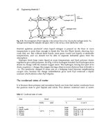
Fig. 11.1. The left-hand part of the iron–carbon phase diagram. There are five phases in the Fe–Fe
3
C
system:
L
, d, g, a and Fe
3
C (see Table 11.1).
Atomic
packing
d.r.p.
b.c.c.
f.c.c.
b.c.c.
Complex
Table 11.1 Phases in the Fe–Fe

3
C system
Phase
Liquid
d
g(also called “austenite”)
a(also called “ferrite”)
Fe
3
C (also called “iron
carbide” or “cementite”)
Description and comments
Liquid solution of C in Fe.
Random interstitial solid solution of C in b.c.c. Fe. Maximum
solubility of 0.08 wt% C occurs at 1492°C. Pure d Fe is the
stable polymorph between 1391°C and 1536°C (see Fig. 2.1).
Random interstitial solid solution of C in f.c.c. Fe. Maximum
solubility of 1.7 wt% C occurs at 1130°C. Pure g Fe is the stable
polymorph between 914°C and 1391°C (see Fig. 2.1).
Random interstitial solid solution of C in b.c.c. Fe. Maximum
solubility of 0.035 wt% C occurs at 723°C. Pure a Fe is the
stable polymorph below 914°C (see Fig. 2.1).
A hard and brittle chemical compound of Fe and C containing
25 atomic % (6.7 wt%) C.
Steels: I – carbon steels 115
Table 11.2 Composite structures produced during the slow cooling of Fe–C alloys
Name of structure Description and comments
Pearlite The composite eutectoid structure of alternating plates of a and Fe
3
C produced when

g containing 0.80 wt% C is cooled below 723°C (see Fig. 6.7 and Phase Diagrams
p. 344). Pearlite nucleates at g grain boundaries. It occurs in low, medium and high
carbon steels. It is sometimes, quite wrongly, called a phase. It is not a phase but is a
mixture
of the two separate phases a and Fe
3
C in the proportions of 88.5% by weight
of a to 11.5% by weight of Fe
3
C. Because grains are single crystals it is
wrong
to say
that Pearlite forms in grains: we say instead that it forms in
nodules
.
Ledeburite The composite eutectic structure of alternating plates of g and Fe
3
C produced when
liquid containing 4.3 wt% C is cooled below 1130°C. Again,
not
a phase! Ledeburite
only occurs during the solidification of cast irons, and even then the g in ledeburite
will transform to a + Fe
3
C at 723°C.
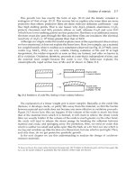
Fig. 11.2. Microstructures during the slow cooling of pure iron from the hot working temperature.
Figures 11.2–11.6 show how the room temperature microstructure of carbon steels
depends on the carbon content. The limiting case of pure iron (Fig. 11.2) is straight-
forward: when
γ

iron cools below 914°C
α
grains nucleate at
γ
grain boundaries and the
microstructure transforms to
α
. If we cool a steel of eutectoid composition (0.80 wt%
C) below 723°C pearlite nodules nucleate at grain boundaries (Fig. 11.3) and the micro-
structure transforms to pearlite. If the steel contains less than 0.80% C (a hypoeutectoid
steel) then the
γ
starts to transform as soon as the alloy enters the
α
+
γ
field (Fig. 11.4).
“Primary”
α
nucleates at
γ
grain boundaries and grows as the steel is cooled from A
3
116 Engineering Materials 2
Fig. 11.3. Microstructures during the slow cooling of a eutectoid steel from the hot working temperature. As
a point of detail, when pearlite is cooled to room temperature, the concentration of carbon in the a decreases
slightly, following the a/a + Fe
3
C boundary. The excess carbon reacts with iron at the a–Fe
3

C interfaces to
form more Fe
3
C. This “plates out” on the surfaces of the existing Fe
3
C plates which become very slightly
thicker. The composition of Fe
3
C is independent of temperature, of course.
Fig. 11.4. Microstructures during the slow cooling of a hypoeutectoid steel from the hot working temperature.
A
3
is the standard labelling for the temperature at which a first appears, and A
1
is standard for the eutectoid
temperature.
Hypo
eutectoid means that the carbon content is
below
that of a eutectoid steel (in the same sense
that hypodermic means “under the skin”!).
Steels: I – carbon steels 117
Fig. 11.5. Microstructures during the slow cooling of a hypereutectoid steel. A
cm
is the standard labelling for
the temperature at which Fe
3
C first appears.
Hyper
eutectoid means that the carbon content is

above
that of a
eutectoid steel (in the sense that a hyperactive child has an above-normal activity!).
Fig. 11.6. Room temperature microstructures in slowly cooled steels of different carbon contents. (a) The
proportions by weight of the different
phases
. (b) The proportions by weight of the different
structures
.
118 Engineering Materials 2
to A
1
. At A
1
the remaining
γ
(which is now of eutectoid composition) transforms to
pearlite as usual. The room temperature microstructure is then made up of primary
α
+ pearlite. If the steel contains more than 0.80% C (a hypereutectoid steel) then we get a
room-temperature microstructure of primary Fe
3
C plus pearlite instead (Fig. 11.5).
These structural differences are summarised in Fig. 11.6.
Mechanical properties of normalised carbon steels
Figure 11.7 shows how the mechanical properties of normalised carbon steels change
with carbon content. Both the yield strength and tensile strength increase linearly with
carbon content. This is what we would expect: the Fe
3
C acts as a strengthening phase,

and the proportion of Fe
3
C in the steel is linear in carbon concentration (Fig. 11.6a).
The ductility, on the other hand, falls rapidly as the carbon content goes up (Fig. 11.7)
because the
α
–Fe
3
C interfaces in pearlite are good at nucleating cracks.
Fig. 11.7. Mechanical properties of normalised carbon steels.
Quenched and tempered carbon steels
We saw in Chapter 8 that, if we cool eutectoid
γ
to 500°C at about 200°C s
−1
, we will
miss the nose of the C-curve. If we continue to cool below 280°C the unstable
γ
will
begin to transform to martensite. At 220°C half the
γ
will have transformed to martensite.
And at –50°C the steel will have become completely martensitic. Hypoeutectoid and
hypereutectoid steels can be quenched to give martensite in exactly the same way
(although, as Fig. 11.8 shows, their C-curves are slightly different).
Figure 11.9 shows that the hardness of martensite increases rapidly with carbon
content. This, again, is what we would expect. We saw in Chapter 8 that martensite is
a supersaturated solid solution of C in Fe. Pure iron at room temperature would be
b.c.c., but the supersaturated carbon distorts the lattice, making it tetragonal
Steels: I – carbon steels 119

Fig. 11.8. TTT diagrams for (a) eutectoid, (b) hypoeutectoid and (c) hypereutectoid steels. (b) and (c) show
(dashed lines) the C-curves for the formation of primary a and Fe
3
C respectively. Note that, as the carbon
content increases, both
M
S
and
M
F

decrease
.
Fig. 11.9. The hardness of martensite increases with carbon content because of the increasing distortion of
the lattice.
120 Engineering Materials 2
Fig. 11.10. Changes during the tempering of martensite. There is a large driving force trying to make the
martensite transform to the equilibrium phases of a + Fe
3
C. Increasing the temperature gives the atoms more
thermal energy, allowing the transformation to take place.
(Fig. 11.9). The distortion increases linearly with the amount of dissolved carbon
(Fig. 11.9); and because the distortion is what gives martensite its hardness then this,
too, must increase with carbon content.
Although 0.8% carbon martensite is very hard, it is also very brittle. You can quench
a 3 mm rod of tool steel into cold water and then snap it like a carrot. But if you temper
martensite (reheat it to 300–600°C) you can regain the lost toughness with only a
moderate sacrifice in hardness. Tempering gives the carbon atoms enough thermal
energy that they can diffuse out of supersaturated solution and react with iron to form
small closely spaced precipitates of Fe

3
C (Fig. 11.10). The lattice relaxes back to the
undistorted b.c.c. structure of equilibrium
α
, and the ductility goes up as a result. The
Fe
3
C particles precipitation-harden the steel and keep the hardness up. If the steel is
Steels: I – carbon steels 121
over-tempered, however, the Fe
3
C particles coarsen (they get larger and further apart)
and the hardness falls. Figure 11.11 shows the big improvements in yield and tensile
strength that can be obtained by quenching and tempering steels in this way.
Cast irons
Alloys of iron containing more than 1.7 wt% carbon are called cast irons. Carbon
lowers the melting point of iron (see Fig. 11.1): a medium-carbon steel must be heated
to about 1500°C to melt it, whereas a 4% cast iron is molten at only 1160°C. This is why
cast iron is called cast iron: it can be melted with primitive furnaces and can be cast
into intricate shapes using very basic sand casting technology. Cast iron castings have
been made for hundreds of years.* The Victorians used cast iron for everything they
could: bridges, architectural beams and columns, steam-engine cylinders, lathe beds,
even garden furniture. But most cast irons are brittle and should not be used where
they are subjected to shock loading or high tensile stresses. When strong castings are
needed, steel can be used instead. But it is only within the last 100 years that steel
castings have come into use; and even now they are much more expensive than cast
iron.
There are two basic types of cast iron: white, and grey. The phases in white iron are
α
and Fe

3
C, and it is the large volume fraction of Fe
3
C that makes the metal brittle. The
name comes from the silvery appearance of the fracture surface, due to light being
reflected from cleavage planes in the Fe
3
C. In grey iron much of the carbon separates
Fig. 11.11. Mechanical properties of quenched-and-tempered steels. Compare with Fig. 11.7.
* The world’s first iron bridge was put up in 1779 by the Quaker ironmaster Abraham Darby III. Spanning
the River Severn in Shropshire the bridge is still there; the local village is now called Ironbridge. Another
early ironmaster, the eccentric and ruthless “iron-mad” Wilkinson, lies buried in an iron coffin surmounted
by an iron obelisk. He launched the world’s first iron ship and invented the machine for boring the cylinders
of James Watt’s steam engines.
122 Engineering Materials 2
out as elemental carbon (graphite) rather than Fe
3
C. Grey irons contain ≈2 wt% Si: this
alters the thermodynamics of the system and makes iron–graphite more stable than
iron–Fe
3
C. If you cut a piece of grey iron with a hacksaw the graphite in the sawdust
will turn your fingers black, and the cut surface will look dark as well, giving grey iron
its name. It is the graphite that gives grey irons their excellent wear properties – in fact
grey iron is the only metal which does not “scuff” or “pick up” when it runs on itself.
The properties of grey iron depend strongly on the shape of the graphite phase. If it is
in the form of large flakes, the toughness is low because the flakes are planes of
weakness. If it is in the form of spheres (spheroidal-graphite, or “SG”, iron) the tough-
ness is high and the iron is surprisingly ductile. The graphite in grey iron is normally
flaky, but SG irons can be produced if cerium or magnesium is added. Finally, some

grey irons can be hardened by quenching and tempering in just the way that carbon
steels can. The sliding surfaces of high-quality machine tools (lathes, milling machines,
etc.) are usually hardened in this way, but in order to avoid distortion and cracking only
the surface of the iron is heated to red heat (in a process called “induction hardening”).
Some notes on the TTT diagram
The C-curves of TTT diagrams are determined by quenching a specimen to a given
temperature, holding it there for a given time, and quenching to room temperature
(Fig. 11.12). The specimen is then sectioned, polished and examined in the microscope.
The percentage of Fe
3
C present in the sectioned specimen allows one to find out how
far the
γ
→
α
+ Fe
3
C transformation has gone (Fig. 11.12). The complete set of C-curves
Fig. 11.12. C-curves are determined using quench–hold–quench sequences.
Steels: I – carbon steels 123
can be built up by doing a large number of experiments at different temperatures and
for different times. In order to get fast enough quenches, thin specimens are quenched
into baths of molten salt kept at the various hold temperatures. A quicker alternative
to quenching and sectioning is to follow the progress of the transformation with a
high-resolution dilatometer: both
α
and Fe
3
C are less dense than
γ

and the extent of the
expansion observed after a given holding time tells us how far the transformation has
gone.
When the steel transforms at a high temperature, with little undercooling, the pearlite
in the steel is coarse – the plates in any nodule are relatively large and widely spaced.
At slightly lower temperatures we get fine pearlite. Below the nose of the C-curve the
transformation is too fast for the Fe
3
C to grow in nice, tidy plates. It grows instead as
isolated stringers to give a structure called “upper bainite” (Fig. 11.12). At still lower
temperatures the Fe
3
C grows as tiny rods and there is evidence that the
α
forms by a
displacive transformation (“lower bainite”). The decreasing scale of the microstructure
with increasing driving force (coarse pearlite → fine pearlite → upper bainite → lower
bainite in Fig. 11.12) is an example of the general rule that, the harder you drive a
transformation, the finer the structure you get.
Because C-curves are determined by quench–hold–quench sequences they can, strictly
speaking, only be used to predict the microstructures that would be produced in a steel
subjected to a quench–hold–quench heat treatment. But the curves do give a pretty good
indication of the structures to expect in a steel that has been cooled continuously. For really
accurate predictions, however, continuous cooling diagrams are available (see the literature of
the major steel manufacturers).
The final note is that pearlite and bainite only form from undercooled
γ
. They never
form from martensite. The TTT diagram cannot therefore be used to tell us anything
about the rate of tempering in martensite.

Further reading
K. J. Pascoe, An Introduction to the Properties of Engineering Materials, Van Nostrand Reinhold,
1978.
R. W. K. Honeycombe and H. K. D. H. Bhadeshia, Steels: Microstructure and Properties, 2nd
edition, Arnold, 1995.
R. Fifield, “Bedlam comes alive again”, in New Scientist, 29 March 1973, pp. 722–725. Article on
the archaeology of the historic industrial complex at Ironbridge, U.K.
D. T. Llewellyn, Steels – Metallurgy and Applications, 2nd edition, Butterworth-Heinemann, 1994.
Problems
11.1 The figure below shows the isothermal transformation diagram for a coarse-grained,
plain-carbon steel of eutectoid composition. Samples of the steel are austenitised
at 850°C and then subjected to the quenching treatments shown on the diagram.
Describe the microstructure produced by each heat treatment.
124 Engineering Materials 2
11.2 You have been given samples of the following materials:
(a) Pure iron.
(b) 0.3 wt% carbon steel.
(c) 0.8 wt% carbon steel.
(d) 1.2 wt% carbon steel.
Sketch the structures that you would expect to see if you looked at polished
sections of the samples under a reflecting light microscope. Label the phases, and
any other features of interest. You may assume that each specimen has been
cooled moderately slowly from a temperature of 1100°C.
11.3 The densities of pure iron and iron carbide at room temperature are 7.87 and
8.15 Mg m
−3
respectively. Calculate the percentage by volume of a and Fe
3
C in
pearlite.

Answers: α, 88.9%; Fe
3
C, 11.1%.
·
·
700
600
500
400
300
200
100
0
–100
1
10
10
2
10
3
10
4
Time(s)
M
F
M
50
M
S
a

b
1%
50% 99%
d
cf
e
Temperature (˚C)
·
·
·
·
·
·
·
·
·
·
Steels: II – alloy steels 125
Chapter 12
Steels: II – alloy steels
Introduction
A small, but important, sector of the steel market is that of the alloy steels: the low-
alloy steels, the high-alloy “stainless” steels and the tool steels. Alloying elements are
added to steels with four main aims in mind:
(a) to improve the hardenability of the steel;
(b) to give solution strengthening and precipitation hardening;
(c) to give corrosion resistance;
(d) to stabilise austenite, giving a steel that is austenitic (f.c.c.) at room temperature.
Hardenability
We saw in the last chapter that carbon steels could be strengthened by quenching and

tempering. To get the best properties we must quench the steel past the nose of the C-
curve. The cooling rate that just misses the nose is called the critical cooling rate (CCR).
If we cool at the critical rate, or faster, the steel will transform to 100% martensite.* The
CCR for a plain carbon steel depends on two factors – carbon content and grain size.
We have already seen (in Chapter 8) that adding carbon decreases the rate of the
diffusive transformation by orders of magnitude: the CCR decreases from ≈10
5
°C s
−1
for pure iron to ≈200°C s
−1
for 0.8% carbon steel (see Fig. 12.1). We also saw in Chap-
ter 8 that the rate of a diffusive transformation was proportional to the number of
nuclei forming per m
3
per second. Since grain boundaries are favourite nucleation
sites, a fine-grained steel should produce more nuclei than a coarse-grained one. The
fine-grained steel will therefore transform more rapidly than the coarse-grained steel,
and will have a higher CCR (Fig. 12.1).
Quenching and tempering is usually limited to steels containing more than about
0.1% carbon. Figure 12.1 shows that these must be cooled at rates ranging from 100 to
2000°C s
−1
if 100% martensite is to be produced. There is no difficulty in transforming the
surface of a component to martensite – we simply quench the red-hot steel into a bath
of cold water or oil. But if the component is at all large, the surface layers will tend to
insulate the bulk of the component from the quenching fluid. The bulk will cool more
slowly than the CCR and will not harden properly. Worse, a rapid quench can create
shrinkage stresses which are quite capable of cracking brittle, untempered martensite.
These problems are overcome by alloying. The entire TTT curve is shifted to the

right by adding a small percentage of the right alloying element to the steel – usually
* Provided, of course, that we continue to cool the steel down to the martensite finish temperature.
126 Engineering Materials 2
Fig. 12.1. The effect of carbon content and grain size on the critical cooling rate.
Fig. 12.2. Alloying elements make steels more hardenable.
molybdenum (Mo), manganese (Mn), chromium (Cr) or nickel (Ni) (Fig. 12.2). Numer-
ous low-alloy steels have been developed with superior hardenability – the ability to
form martensite in thick sections when quenched. This is one of the reasons for adding
the 2–7% of alloying elements (together with 0.2–0.6% C) to steels used for things like
crankshafts, high-tensile bolts, springs, connecting rods, and spanners. Alloys with
lower alloy contents give martensite when quenched into oil (a moderately rapid
quench); the more heavily alloyed give martensite even when cooled in air. Having
formed martensite, the component is tempered to give the desired combination of
strength and toughness.
Hardenability is so important that a simple test is essential to measure it. The Jominy
end-quench test, though inelegant from a scientific standpoint, fills this need. A bar
100 mm long and 25.4 mm in diameter is heated and held in the austenite field. When
all the alloying elements have gone into solution, a jet of water is sprayed onto one
end of the bar (Fig. 12.3). The surface cools very rapidly, but sections of the bar behind
Steels: II – alloy steels 127
Fig. 12.3. The Jominy end-quench test for hardenability.
Fig. 12.4. Jominy test on a steel of high hardenability.
the quenched surface cool progressively more slowly (Fig. 12.3). When the whole bar
is cold, the hardness is measured along its length. A steel of high hardenability will
show a uniform, high hardness along the whole length of the bar (Fig. 12.4). This is
because the cooling rate, even at the far end of the bar, is greater than the CCR; and the
whole bar transforms to martensite. A steel of medium hardenability gives quite dif-
ferent results (Fig. 12.5). The CCR is much higher, and is only exceeded in the first few
centimetres of the bar. Once the cooling rate falls below the CCR the steel starts to
transform to bainite rather than martensite, and the hardness drops off rapidly.

128 Engineering Materials 2
Fig. 12.5. Jominy test on a steel of medium hardenability. M = martensite, B = bainite, F = primary ferrite,
P = pearlite.
Solution hardening
The alloying elements in the low-alloy steels dissolve in the ferrite to form a substitutional
solid solution. This solution strengthens the steel and gives useful additional strength.
The tool steels contain large amounts of dissolved tungsten (W) and cobalt (Co) as well,
to give the maximum feasible solution strengthening. Because the alloying elements
have large solubilities in both ferrite and austenite, no special heat treatments are
needed to produce good levels of solution hardening. In addition, the solution-hardening
component of the strength is not upset by overheating the steel. For this reason, low-
alloy steels can be welded, and cutting tools can be run hot without affecting the
solution-hardening contribution to their strength.
Precipitation hardening
The tool steels are an excellent example of how metals can be strengthened by precipita-
tion hardening. Traditionally, cutting tools have been made from 1% carbon steel
with about 0.3% of silicon (Si) and manganese (Mn). Used in the quenched and tem-
pered state they are hard enough to cut mild steel and tough enough to stand up to the
shocks of intermittent cutting. But they have one serious drawback. When cutting
tools are in use they become hot: woodworking tools become warm to the touch, but
metalworking tools can burn you. It is easy to “run the temper” of plain carbon
Steels: II – alloy steels 129
metalworking tools, and the resulting drop in hardness will destroy the cutting edge.
The problem can be overcome by using low cutting speeds and spraying the tool with
cutting fluid. But this is an expensive solution – slow cutting speeds mean low produc-
tion rates and expensive products. A better answer is to make the cutting tools out of
high-speed steel. This is an alloy tool steel containing typically 1% C, 0.4% Si, 0.4% Mn,
4% Cr, 5% Mo, 6% W, 2% vanadium (V) and 5% Co. The steel is used in the quenched
and tempered state (the Mo, Mn and Cr give good hardenability) and owes its strength
to two main factors: the fine dispersion of Fe

3
C that forms during tempering, and the
solution hardening that the dissolved alloying elements give.
Interesting things happen when this high-speed steel is heated to 500–600°C. The
Fe
3
C precipitates dissolve and the carbon that they release combines with some of the
dissolved Mo, W and V to give a fine dispersion of Mo
2
C, W
2
C and VC precipitates.
This happens because Mo, W and V are strong carbide formers. If the steel is now cooled
back down to room temperature, we will find that this secondary hardening has made it
even stronger than it was in the quenched and tempered state. In other words, “run-
ning the temper” of a high-speed steel makes it harder, not softer; and tools made out
of high-speed steel can be run at much higher cutting speeds (hence the name).
Corrosion resistance
Plain carbon steels rust in wet environments and oxidise if heated in air. But if chro-
mium is added to steel, a hard, compact film of Cr
2
O
3
will form on the surface and this
will help to protect the underlying metal. The minimum amount of chromium needed
to protect steel is about 13%, but up to 26% may be needed if the environment is
particularly hostile. The iron–chromium system is the basis for a wide range of stain-
less steels.
Stainless steels
The simplest stainless alloy contains just iron and chromium (it is actually called

stainless iron, because it contains virtually no carbon). Figure 12.6 shows the Fe–Cr
phase diagram. The interesting thing about this diagram is that alloys containing
ը13% Cr have a b.c.c. structure all the way from 0 K to the melting point. They do not
enter the f.c.c. phase field and cannot be quenched to form martensite. Stainless irons
containing ը13% Cr are therefore always ferritic.
Hardenable stainless steels usually contain up to 0.6% carbon. This is added in order
to change the Fe–Cr phase diagram. As Fig. 12.7 shows, carbon expands the
γ
field so
that an alloy of Fe–15% Cr, 0.6% C lies inside the
γ
field at 1000°C. This steel can be
quenched to give martensite; and the martensite can be tempered to give a fine disper-
sion of alloy carbides.
These quenched and tempered stainless steels are ideal for things like non-rusting
ball-bearings, surgical scalpels and kitchen knives.*
* Because both ferrite and martensite are magnetic, kitchen knives can be hung up on a strip magnet
screwed to the kitchen wall.
130 Engineering Materials 2
Fig. 12.6. The Fe–Cr phase diagram.
Many stainless steels, however, are austenitic (f.c.c.) at room temperature. The most
common austenitic stainless, “18/8”, has a composition Fe–0.1% C, 1% Mn, 18% Cr,
8% Ni. The chromium is added, as before, to give corrosion resistance. But nickel is
added as well because it stabilises austenite. The Fe–Ni phase diagram (Fig. 12.8) shows
why. Adding nickel lowers the temperature of the f.c.c.–b.c.c. transformation from
914°C for pure iron to 720°C for Fe–8% Ni. In addition, the Mn, Cr and Ni slow the
diffusive f.c.c.–b.c.c. transformation down by orders of magnitude. 18/8 stainless steel
can therefore be cooled in air from 800°C to room temperature without transforming
to b.c.c. The austenite is, of course, unstable at room temperature. However, diffu-
sion is far too slow for the metastable austenite to transform to ferrite by a diffusive

mechanism. It is, of course, possible for the austenite to transform displacively to give
Fig. 12.7. Simplified phase diagram for the Fe–Cr–0.6% C system.
Steels: II – alloy steels 131
martensite. But the large amounts of Cr and Ni lower the M
S
temperature to ≈0°C. This
means that we would have to cool the steel well below 0°C in order to lose much
austenite.
Austenitic steels have a number of advantages over their ferritic cousins. They are
tougher and more ductile. They can be formed more easily by stretching or deep
drawing. Because diffusion is slower in f.c.c. iron than in b.c.c. iron, they have better
creep properties. And they are non-magnetic, which makes them ideal for instruments
like electron microscopes and mass spectrometers. But one drawback is that austenitic
steels work harden very rapidly, which makes them rather difficult to machine.
Background reading
M. F. Ashby and D. R. H. Jones, Engineering Materials I, 2nd edition, Butterworth-Heinemann,
1996, Chapters 21, 22, 23 and 24.
Further reading
K. J. Pascoe, An Introduction to the Properties of Engineering Materials, Van Nostrand Reinhold,
1978.
R. W. K. Honeycombe and H. K. D. H. Bhadeshia, Steels: Microstructure and Properties, 2nd
edition, Arnold, 1995.
Smithells’ Metals Reference Book, 7th edition, Butterworth-Heinemann, 1992 (for data on uses and
compositions of steels, and iron-based phase diagrams).
A. H. Cottrell, An Introduction to Metallurgy, 2nd edition, Arnold, 1975.
D. T. Llewellyn, Steels – Metallurgy and Applications, 2nd edition, Butterworth-Heinemann, 1994.
Fig. 12.8. The Fe–Ni phase diagram.
132 Engineering Materials 2
Problems
12.1 Explain the following.

(a) The critical cooling rate (CCR) is approximately 700°C s
–1
for a fine-grained
0.6% carbon steel, but is only around 30°C s
–1
for a coarse-grained 0.6% carbon
steel.
(b) A stainless steel containing 18% Cr has a bcc structure at room temperature,
whereas a stainless steel containing 18% Cr plus 8% Ni has an fcc structure at
room temperature.
(c) High-speed steel cutting tools retain their hardness to well above the tem-
perature at which the initial martensitic structure has become over-tempered.
12.2 A steel shaft 40 mm in diameter is to be hardened by austenitising followed by
quenching into cold oil. The centre of the bar must be 100% martensite. The
following table gives the cooling rate at the centre of an oil quenched bar as a
function of bar diameter.
Bar diameter (mm) Cooling rate (°C s
−
1
)
500 0.17
100 2.5
20 50
5 667
It is proposed to make the shaft from a NiCrMo low-alloy steel. The critical
cooling rates of NiCrMo steels are given quite well by the empirical equation

log ( ) . .
()
.

10
1
43 327
16
CCR in C s C
Mn Cr Mo Ni
°=− −
++ +
−
where the symbol given for each element denotes its weight percentage. Which of
the following steels would be suitable for this application?
[Hint: there is a log–log relationship between bar diameter and cooling rate.]
Answer: Steels B, C, D, G.
Steel Weight percentages
CMnCrMoNi
A 0.30 0.80 0.50 0.20 0.55
B 0.40 0.60 1.20 0.30 1.50
C 0.36 0.70 1.50 0.25 1.50
D 0.40 0.60 1.20 0.15 1.50
E 0.41 0.85 0.50 0.25 0.55
F 0.40 0.65 0.75 0.25 0.85
G 0.40 0.60 0.65 0.55 2.55
Case studies in steels 133
Chapter 13
Case studies in steels
Metallurgical detective work after a boiler explosion
The first case study shows how a knowledge of steel microstructures can help us trace
the chain of events that led to a damaging engineering failure.
The failure took place in a large water-tube boiler used for generating steam in a
chemical plant. The layout of the boiler is shown in Fig. 13.1. At the bottom of the

boiler is a cylindrical pressure vessel – the mud drum – which contains water and
sediments. At the top of the boiler is the steam drum, which contains water and steam.
The two drums are connected by 200 tubes through which the water circulates. The
tubes are heated from the outside by the flue gases from a coal-fired furnace. The
water in the “hot” tubes moves upwards from the mud drum to the steam drum, and
the water in the “cool” tubes moves downwards from the steam drum to the mud
drum. A convection circuit is therefore set up where water circulates around the boiler
and picks up heat in the process. The water tubes are 10 m long, have an outside
diameter of 100 mm and are 5 mm thick in the wall. They are made from a steel of
composition Fe–0.18% C, 0.45% Mn, 0.20% Si. The boiler operates with a working
pressure of 50 bar and a water temperature of 264°C.
Fig. 13.1. Schematic of water-tube boiler.
134 Engineering Materials 2
Fig. 13.2. Schematic of burst tube.
In the incident some of the “hot” tubes became overheated, and started to bulge.
Eventually one of the tubes burst open and the contents of the boiler were discharged
into the environment. No one was injured in the explosion, but it took several months
to repair the boiler and the cost was heavy. In order to prevent another accident, a
materials specialist was called in to examine the failed tube and comment on the
reasons for the failure.
Figure 13.2 shows a schematic diagram of the burst tube. The first operation was to
cut out a 20 mm length of the tube through the centre of the failure. One of the cut
surfaces of the specimen was then ground flat and tested for hardness. Figure 13.3
shows the data that were obtained. The hardness of most of the section was about
2.2 GPa, but at the edges of the rupture the hardness went up to 4 GPa. This indicates
(see Fig. 13.3) that the structure at the rupture edge is mainly martensite. However,
away from the rupture, the structure is largely bainite. Hardness tests done on a spare
boiler tube gave only 1.5 GPa, showing that the failed tube would have had a ferrite
+ pearlite microstructure to begin with.
In order to produce martensite and bainite the tube must have been overheated to at

least the A
3
temperature of 870°C (Fig. 13.4). When the rupture occurred the rapid
outrush of boiler water and steam cooled the steel rapidly down to 264°C. The cooling
rate was greatest at the rupture edge, where the section was thinnest: high enough to
quench the steel to martensite. In the main bulk of the tube the cooling rate was less,
which is why bainite formed instead.
The hoop stress in the tube under the working pressure of 50 bar (5 MPa) is 5 MPa
× 50 mm/5 mm = 50 MPa. Creep data indicate that, at 900°C and 50 MPa, the steel
should fail after only 15 minutes or so. In all probability, then, the failure occurred by
creep rupture during a short temperature excursion to at least 870°C.
How was it that water tubes reached such high temperatures? We can give two
probable reasons. The first is that “hard” feed water will – unless properly treated –
Case studies in steels 135
Fig. 13.3. The hardness profile of the tube.
Fig. 13.4. Part of the iron–carbon phase diagram.