Modern Developments in X-Ray and Neutron Optics Episode 2 pptx
Bạn đang xem bản rút gọn của tài liệu. Xem và tải ngay bản đầy đủ của tài liệu tại đây (2.43 MB, 40 trang )
20 F. Sch¨afers
The direction cosines are transformed correspondingly:
α
S
= D
˜x
(θ) D
z
(χ) α
S
, (2.10)
and finally
⎛
⎝
l
S
m
S
n
S
⎞
⎠
=
⎛
⎝
l
s
cos χ − m
s
sin χ
l
s
sin χ cos θ + m
s
cos χ cos θ
l
s
sin χ sin θ + m
s
cos χ sin θ
⎞
⎠
. (2.11)
In the new coordinate system the ray is described by
⎛
⎝
x
y
z
⎞
⎠
(t)=
⎛
⎝
x
S
y
S
z
S
⎞
⎠
+ t
⎛
⎝
l
S
m
S
n
S
⎞
⎠
(2.12)
2.5.4 Misalignment
A six-dimensional misalignment of an optical element can be taken into
account: three translations of the coordinate system by δx, δy and δz and
three rotations by the misorientation angles δχ (x-y plane), δϕ (x-z plane)
and δψ (y-z plane). Since the rotations are not commutative, the coordinate
system is first rotated by these angles in the given order and then translated.
For the outgoing ray to be described in the non-misaligned system, the coor-
dinate system is backtransformed (in reverse order). Thus, the optical axis
remains unaffected by the misalignment.
2.5.5 Second-Order Surfaces
Optical elements are described by the general equation for second-order
surfaces:
F (x, y, z)=a
11
x
2
+ a
22
y
2
+ a
33
z
2
+2a
12
xy +2a
13
xz
+2a
23
yz +2a
14
x +2a
24
y +2a
34
z + a
44
=0.
(2.13)
This description refers to a right-handed coordinate system attached to the
centre of the mirror with its surface in x-z plane, and y-axis points to the
normal). This coordinate system is used for the optical elements PL
ane,
CO
ne, CY linder and SP here.
Note that for the elements EL
lipsoid and PA raboloid acoordinatesystem
is used, which again is attached to the centre of the mirror (with x-axis on the
surface), but the z-axis is parallel to the symmetry axis of this element for an
easier description in terms of the a
ij
parameters (see Figs. 2.9 and 2.10). The
a
ij
-values of Table 2.2 are given for this system. Thus, the rotation angle of
the coordinate system from source to element is here θ+α (EL)and2θ (PA),
respectively, θ being the grazing incidence angle and α the tangent angle on
the ellipse.
2 The BESSY Raytrace Program RAY 21
a
b
Y
Ell
Z
Ell
Focus
X
Ell
Y
Mi
Z
Mi
Y
Ell
Z
Ell
Y
o
Z
o
Z
So
Y
So
X
So
X
Im
Z
Im
Y
Im
α
Θ
α
Source
Fig. 2.9. Ellipsoid: definitions and coordinate systems
θ
θ
θ
X
Pa
X
So
Z
Pa
Z
Mi
Z
Pa
Z
o
Y
Mi
Z
So
Source
Directrix
Y
So
Y
Pa
Y
Pa
Y
Im
Z
Im
X
Im
P
Fig. 2.10. Paraboloid: Definitions and coordinate systems
The individual surfaces are described by the following equations:
• Plane y =0
• Cylinder(in z −dir.) x
2
+ y
2
=0
• Cylinder(in x − dir.) y
2
+ z
2
=0
• Sphere x
2
+(y −R)
2
+ z
2
− R
2
=0
• Ellipsoid x
2
/C
2
+(y −y
0
)
2
/B
2
+(z −z
0
)
2
/A
2
− 1=0
• Paraboloid x
2
/C
2
+(y −y
0
)
2
/B
2
− 2P (z −z
0
)=0
(2.14)
Alternatively to the input of suitable parameters, such as mirror radii or
half axes of ellipses, in an experts modus (EO), the a
ij
parameters can be
directly given, such that any second-order surface, whatever shape it has, can
be simulated.
22 F. Sch¨afers
Tab le 2.2. Parameters of the second-order optical elements
Name PM CY CO SP EL PA
a
11
0 1/0 1 − c
m
1 B
2
/C
2
P
2
/C
2
a
22
01 1− 2c
m
11 1
a
33
0 0/1 0 1 B
2
/A
2
0
a
12
00 0 0 0 0
a
13
00 0 0 0 0
a
23
00
c
m
− c
2
m
00 0
a
14
00 0 0 0
a
24
−1 ρ · sign −a
23
R
√
c
m
−
z
m
2
R · sign −y
0
−y
0
a
34
000z
0
B
2
/A
2
−P
a
44
00 0 0 y
2
0
+ z
2
0
B
2
/A
2
− B
2
y
2
0
− 2Pz
0
− P
2
Sign
(concave/convex)
01/−11/−11/−11 1
F
x
− (a
11
x + a
12
y +
a
13
z + a
14
)
0 −x/0 −x −a
11
x −a
11
x
F
y
− (a
22
y · sign +
a
12
xa
23
z + a
24
)
1 ρ · sign R · sign y
0
− yy
0
− y
F
z
− (a
33
z + a
13
x +
a
23
y + a
34
)
00/−z −z −(z
0
+ z)(B/A)
2
P
z
0
= A
2
/B
2
y
0
tan(α) z
0
= f cos(α, β) · sig
y
0
= r
a
sin(θ − α) y
0
= f sin(2 α, β)
tan(α)=tan(θ) P =2f sin
2
(θ)sig
(r
a
− r
b
)/(r
a
+ r
b
)
ρ:radius R, ρ:radii R: radius f: mirror–source/focus–dist.
z
m
: mirror
length c
m
=
(r−ρ)
z
m
2
A, B, C half axes in z,y,x-dir;
r
a
,r
b
: mirror to focus 1,2; θ:
grazing angle of central ray; α:
tangent angle
C: halfpar. in x;Sig=±1; f.
collimation/focussing; θ:grazing
angle of central ray; α, β =2θ, 0
(coll); α, β =0, 2θ (foc.)
Plane Ell.: C = infty.; Rotational
Ell.: B = C<>A; Ellipsoid:
A = B = C; Sphere: A = B = C
Plane P : C = infty.; Rotational
P : C = P; Elliptical P : C = P
2 The BESSY Raytrace Program RAY 23
2.5.6 Higher-Order Surfaces
A similar expert modus is available for surfaces, which cannot be described
by the second-order equation. The general equation is the following:
F (x, y, z)=a
11
x
2
+signa
22
y
2
+ a
33
z
2
+2a
12
xy +2a
13
xz +2a
23
yz
+2a
14
x +2a
24
y +2a
34
z + a
44
+ b
12
x
2
y + b
21
xy
2
+ b
13
x
2
z + b
31
xz
2
+ b
23
y
2
z + b
32
yz
2
=0
(2.15)
Here, again all a
ij
and b
ij
parameters can be given explicitly by the user to
describe any geometrical surface.
For special higher order surfaces the surface is described by the following
equations.
Toroid
F (x, y, z)=
(R − ρ)+sign(ρ)
ρ
2
− x
2
2
− (y −R)
2
− z
2
= 0 (2.16)
Sign = ±1 for concave/convex curvature.
The surface normal is calculated according to (see Chap. 5.7)
F
x
=
−2x sign(ρ)
ρ
2
− x
2
(R − ρ)+sign(ρ)
ρ
2
− x
2
2
(2.17)
F
y
= −2(y − R) (2.18)
F
z
= −2z. (2.19)
Elliptical Paraboloid
F (x, y, z)=
2fx
2
2f −
z+z
0
cos 2θ
− 2p(z + z
0
) − p
2
=0. (2.20)
Elliptical Toroid
In analogy to a spherical toroid, an elliptical toroid is constructed from an
ellipse (instead of a circle) in the (y, z) plane with small circles of fixed radius
ρ attached in each point perpendicular to the guiding ellipse.
The mathematical description of the surface is based on the description of
a toroid, where in each point of the ellipse a ‘local’ toroid with radius R(z)
and center (y
c
(z),z
c
(z)) is approximated (Fig. 2.11).
Following this description the elliptical toroid surface is given by
F (x, y, z)=0=(z − z
c
(z))
2
+(y − y
c
(z))
2
−
R (z) − ρ +
ρ
2
− x
2
2
(2.21)
24 F. Sch¨afers
α
α
α
R(z
0
,y
0
)
(z
0
,y
0
)
(z
c
,y
c
)
a
b
z
y
x
Fig. 2.11. Construction of an elliptical toroid. The ET is locally approximated by
a conventional spherical toroid with radius R(z)andcenter(z
c
(z),y
c
(z))
with R(z)=a
2
b
2
z
2
a
4
+
a
2
− z
2
a
2
b
2
3
2
=
1
ab
b
2
− a
2
a
2
z
2
+ a
2
3
2
z
c
(z)=z − R(z)sinα(z),
y
c
(z)=y(z)+R(z)cosα(z),
z
c
=1− R
sin α − Rα
cos α,
y
c
= y
+ R
cos α − Rα
sin α,
y(z)=−
b
a
a
2
− z
2
,
α =arctan(y
) = arctan
b
a
z
√
a
2
− z
2
,
y
=
∂y
∂z
=tanα =
b
a
z
√
a
2
− z
2
α
=
∂α
∂z
=
y
1+y
2
,
y
=
∂
2
y
∂z
2
=
ab
(a
2
− z
2
)
3
2
.
The surface normal is given by the partial derivatives
∂F
∂x
=2
x
ρ
2
− x
2
R − ρ +
ρ
2
− x
2
, (2.22)
2 The BESSY Raytrace Program RAY 25
∂F
∂y
=2(y −y
c
), (2.23)
∂F
∂z
=2(z −z
c
(1 − z
c
) − 2y
c
(y − y
c
) − 2R
R − ρ +
ρ
2
− x
2
. (2.24)
2.5.7 Intersection Point
The intersection point (x
M
,y
M
,z
M
) of the ray with the optical element is
determined by solving the quadratic equation in t generated by inserting (2.12)
into (2.13) or (2.15). For the special higher-order surfaces (TO, EP, ET) the
intersection point is determined iteratively.
Then the local surface normal for this intersection point n = n(x
M
,y
M
,z
M
)
is found by calculating the partial derivative of F (x
M
,y
M
,z
M
)
f = ∇F, (2.25)
with the components
f
x
=
∂F
∂x
f
y
= −
∂F
∂y
f
z
=
∂F
∂z
. (2.26)
The local surface normal is then given by the unit vector
n =
⎛
⎝
n
x
n
y
n
z
⎞
⎠
=
1
f
x
2
+ f
y
2
+ f
z
2
⎛
⎝
f
x
f
y
f
z
⎞
⎠
. (2.27)
Whenever the intersection point found is outside the given dimensions of the
optical element, the ray is thrown away as a geometrical loss and the next ray
starts within the source according to Chap. 5.2.
2.5.8 Slope Errors, Surface Profiles
Once the intersection point and the local surface normal is found, these are
the parameters that are modified to include real surfaces as deviations from
the mathematical surface profile, namely figure and finish errors (slope errors,
surface roughness), thermal distortion effects or measured surface profiles.
The surface normal is modified incrementally by rotating the normal
vector in the y-z (meridional plane) and in the x-y plane (sagittal). The
determination of the rotation angles depends on the type of error to be
included.
1. Slope errors, surface roughness: the rotation angles are chosen statistically
(according to the procedure described in Sect. 2.3.1) within a 6σ-width of
the input value for the slope error.
2. Thermal bumps: a gaussian height profile in x-andz-direction with a given
amplitude, and σ-width can be put onto the mirror centre.
26 F. Sch¨afers
3. Cylindrical bending: a cylindrical profile in z-direction (dispersion direc-
tion) with a given amplitude can be superimposed onto the mirror surface.
4. Measured surface profiles, e.g. by a profilometer.
5. Surface profiles calculated separately, e.g. by a finite element analysis
program.
In cases (2–5) the modified mirror is stored in a 251 × 251 surface mesh
which contains the amplitudes (y-coordinates). For cases (2) and (3) this mesh
is calculated within RAY, for the cases (4) and (5) ASCII data files with
surface profilometer data (e.g. LTP or ZEISS M400 [27]) or finite-element-
analysis data (e.g. ANSYS [28]) can be read in. The new y-coordinate of
the intersection point and the local slope are interpolated from such a table
accordingly.
2.5.9 Rays Leaving the Optical Element
For those rays that have survived the interaction with the optical element –
geometrically and within the reflectivity statistics (Chap. 6) – the direction
cosines of the reflected/transmitted/refracted ray (α
2
)=(l
2
,m
2
,n
2
)arecal-
culated from the incident ray (α
1
)=(l
1
,m
1
,n
1
) and the local surface normal
n.
Mirrors
For mirrors and crystals the entrance angle, α, is equal to the exit angle, β.
In vector notation this means that the cross product is
n × (α
2
− α
1
)=0, (2.28)
since the difference vector is parallel to the normal. For the direction cosines
of the reflected ray the result is given by
α
2
= α
1
− 2(n ◦ α
1
)n (2.29)
or in coordinates
l
2
= l
1
− 2n
x
ln
x
+mn
y
+ nn
z
n
x
2
+ n
y
2
+ n
z
2
(2.30)
and, correspondingly, for m
2
and n
2
.
Gratings
The emission angle β for diffraction gratings is obtained by the grating
equation
kλ = d (sin α +sinβ) , (2.31)
k, diffraction order; λ, wavelength; d, grating constant.
2 The BESSY Raytrace Program RAY 27
1. The grating is rotated by δχ = a tan(n
x
/n
y
) around the z-axis and by
δψ = a sin(n
z
) around the x-axis, so that the intersection point is plane
(surface normal parallel to the y-axis). The grating lines are parallel to the
x-direction.
2. Then the direction cosines of the diffracted beam are determined by
⎛
⎝
l
2
m
2
n
2
⎞
⎠
=
⎛
⎜
⎝
l
1
m
2
1
+ n
2
1
− (n
1
− a
1
)
2
n
1
− a
1
⎞
⎟
⎠
, (2.32)
a
1
= k
λ
d
cos δψ.
3. The grating is rotated back to the original position by −δψ and −δχ.
For varied line spacing (VLS) gratings, the local line density n =1/d(l/mm)
as a function of the (x, z)-position is determined by [29]
n = n
0
·
1+2b
2
z +3b
3
z
2
+4b
4
z
3
+2b
5
x +3b
6
x
2
+4b
7
x
3
. (2.33)
Transmitting Optics
For transmitting optics (SL
it, FO il) the direction of the ray is unchanged by
geometry. However, diffraction is taken into account for the case of rectangular
or circular slits by randomly modifying the direction of each ray according to
the probability for a certain direction ϕ
P (ϕ)=
sin u
u
, (2.34)
with u =
πb sinϕ
λ
(b, slit opening; λ, wavelength),
so that for a statistical ensemble of rays a Fraunhofer (rectangular slits) or
bessel pattern (circular slits) appears (see Fig. 2.12). ZO
neplate transmitting
optics are described in [12,13].
Azimuthal Rotation
After successful interaction with the optical element the surviving ray is
described in a coordinate system, which is rotated by the reflection angle
θ and the azimuthal angle χ, such that the z-axis follows once again the
direction of the outgoing central ray as it was for the incident ray. The old
values of the source/mirror points and direction cosines are replaced by these
new ones, so that a new optical element can be attached now in similar way.
28 F. Sch¨afers
Fig. 2.12. Fraunhofer diffraction pattern on a rectangular slit
2.5.10 Image Planes
If the ray has traversed the entire optical system, the intersection points
(x
I
,y
I
) with up to three image planes at the distances z
I
1,2,3
are determined
according to
x
I
y
I
=
x
y
+
1
n
l
m
(z
I
1,2,3
− z). (2.35)
Once a ray reaches the image plane or whenever a ray is lost within the optical
system a new ray is created within the source and the procedure starts all over.
2.5.11 Determination of Focus Position
For the case of imaging systems, if the focus position is to be determined, the
x-andy-coordinates of that ray which has the largest coordinates are stored
along the light beam in the range of the expected focal position (search in a
distance from last OE of +/− ). The so found cross section of the beam
(width and height) is displayed graphically. Since at each position a different
ray may be the outermost one, there may be bumps in this focal curve which
depend on the quality of the imaging. Especially, for optical systems with large
divergences (and thus large optical aberrations) or which include dispersing
elements, this curve is only schematic and serves as a quick check of the focal
properties of the system.
2.5.12 Data Evaluation, Storage and Display
The x, z-coordinates of the intersection point (x, y for source, slits, foils,
zoneplates and image planes) and the angles l, n (l, m, respectively) are stored
into 100 × 100 matrices. These matrices are multichannel arrays, one for the
source, for each optical element and for each image plane, whose dimensions
2 The BESSY Raytrace Program RAY 29
(and with it the pixel size) have been fixed before in a ‘test-raytrace’ run.
They represent the illuminated surface in x-z projection. The corresponding
surface pixel element that has been hit by a ray is increased by 1, so that
intensity profiles and/or heat load can be displayed.
Additionally, the x-andz-coordinates (y, respectively) of the first 10,000
rays are stored in a 10,000x2 ASCII matrix to display footprint patterns of
the optical elements, for point diagrams at the image planes or for further
evaluation outside the program.
2.6 Reflectivity and Polarisation
Not only the geometrical path of the rays is followed, but also the inten-
sity and polarisation properties of each ray are traced throughout an optical
setup. Thus, it is easily possible to preview depolarisation effects throughout
the optical path, or to optimize an optical setup for use as, for example, a
polarisation monitor. For this, each ray is treated individually with a defined
energy and polarisation state.
RAY employs the Stokes formalism for this purpose. The Stokes vector
S =(S
0
,S
1
,S
2
,S
3
) describing the polarisation (S
1
,S
2
: linear, S
3
: circular
polarisation) for each ray is given either as free input parameter or, for dipole
sources, is calculated according to the Schwinger theory. S
0
, the start intensity
of the ray from the source
S
0
=
√
S
1
2
+ S
2
2
+ S
3
2
, is set to 1 for the artificial
sources. It is scaled to a realistic photon flux value for the synchrotron sources
Dipole, Wiggler or the Undulator-File.
The Stokes vector is defined by the following equations:
S
0
=
(E
o
p
)
2
+(E
o
s
)
2
2=1,
S
1
=
(E
o
p
)
2
− (E
o
s
)
2
2=P
l
cos(2δ),
S
2
= E
o
p
E
o
s
cos(φ
p
− φ
s
)=P
l
sin(2δ),
S
3
= −E
o
p
E
o
s
sin(φ
p
− φ
s
)=P
c
, (2.36)
with the two components of the electric field vector defined as
E
p,s
(z,t)=E
o
p,s
exp [i (ωt −kz + φ
p,s
)] . (2.37)
and P
l
,P
c
are the degree of linear and circular polarisation, respectively. δ is
the azimuthal angle of the major axis of the polarisation ellipse. Note that
P
l
= P cos(2ε)
and P
c
= P sin(2ε), (2.38)
with P being the degree of total polarisation and ε the ellipticity of the
polarisation ellipse (tan ε = R
p
/R
s
) .
30 F. Sch¨afers
Tab le 2. 3. Definition of circular polarisation
Phase φ
p−s
90
◦
, −270
◦
−90
◦
, 270
◦
(π/2, −3π/2) (−π/2, 3π/2)
Rotation sense (in time) Clockwise Counter-clockwise
Rotation sense (in space) Counter-clockwise Clockwise
Polarisation (optical def.) R(ight) CP L(eft) CP
Helicity (atomic def.) Negative (σ−) Positive (σ+)
Stokes vector Negative Positive
Tab le 2.4. Physical interaction for the different optical components
Mirrors Gratings Foils Slits Zone-plates Crystals
Fresne l
equations
Diffraction Fresnel
equations
––Dynamic
theory
Reflectivity Efficiency Transmission Transmission Transmission Reflectivity
R
s
,R
p
,Δ
sp
E
s
,E
p
,Δ
sp
T
s
,T
p
,Δ
sp
T
s
,T
p
=1
Δ
sp
=0
T
s
,T
p
=1,
Δ
sp
=0
R
s
,R
p
,Δ
sp
Since the SR is linearly polarised within the electron orbital plane (I
perp
=
0), the plane of linear polarisation is coupled to the x-axis (i.e. horizontal).
Thus, the Stokes vector for SR is defined in our geometry as (see Chap. 3.4)
P
lin
= S
1
=(I
perp
− I
par
)/(I
perp
+ I
par
)=(I
y
− I
x
)/(I
y
+ I
x
)=−1, (2.39)
S
1
= +1 would correspond to a vertical polarisation plane.
For the definition of the circular polarisation the nomenclature of
Westerfeld et al. [30] and Klein/Furtak [31] has been used. This is summarised
in Table 2.3:
For example, for the case of synchrotrons and storage rings, the radiation
that is emitted off-plane, upwards, has negative helicity, right-handed CP
(S
3
= −1), when the electrons are travelling clockwise, as seen from the top.
The modification of the Stokes vector throughout the beamline by inter-
action of the light with the optical surface is described by the following steps
(see e.g. [28]):
(1) Give each ray a start value for the Stokes parameter within the source,
S
ini
, according to input or as calculated for SR sources
(2) Calculate the intensity loss at the first optical element for s- and p-
polarisation geometry and the relative phase, Δ = δ
s
− δ
p
, according
to the physical process involved (see Table 2.4):
• Mirrors, Foils
The optical properties of mirrors, multilayers, filters, gratings and crystals
are calculated from the compilation of atomic scattering factors in the
spectral range from 30 eV to 30 keV [32]. Another data set covers the X-
ray range from 5 up to 50 keV [33]. Additional data for lower energies
down to 1 eV are also available for some elements and molecules [34].
2 The BESSY Raytrace Program RAY 31
10
-3
10
-2
10
-1
10
0
10
1
10
2
Structure factors f
o
, f
H
, f
HC
Cromer f
1
,f
2
(Z=2-92)
Henke (Z=1-92) f
1
, f
2
Palik (Al, Au, C, Cr, Cu, Ir, Ni, Os, Pt, Si n, k)
Molecules: Al
2
O
3
, MgF
2
, Diamond, SiC, SiO
2
n,k
Photon Energy (keV)
Optical data tables for RAY
Fig. 2.13. Data bases used for the calculation of optical properties
A summary of the various data tables available within the program is
given in Fig. 2.13. For compound materials that can be defined by the case
sensitive chemical formula (e.g. MgF
2
), the contributions of the chemical
elements are weighted according to their stochiometry. A tabulated or,
if not available, calculated value for the density is proposed but can be
changed. The surface roughness of mirrors or multilayers is taken into
account according to the Nevot–Croce formalism [35].
All reflection mirrors and transmission foils in an optical setup can
have a multilayer coating (plus an additional top coating). The optical
properties of these structures are calculated in transmission and reflection
geometry by a recursive application of the Fresnel equations. For periodic
multilayers, the layer thickness, the density and the surface roughness
must be specified for each type of interface. For aperiodic structures like
broad-band or supermirrors, the exact structure has to be provided in a
data-file.
• Gratings
For the calculation of (monolayer covered) reflection gratings, a code
developed by Neviere is used [36], which allows for the calculation for
three different grating profiles (sinusoidal, laminar or blazed). In addition
to fixed deviation angle mounts, optionally the incidence angle can be
coupled to the photon energy and the c
ff
factor in the case of a Petersen
32 F. Sch¨afers
SX700 type monochromator (PGM or SGM with a plane pre-mirror which
enables the deviation angle across the grating to be varied).
• Crystals
For crystals the diffraction properties are calculated from the dynamical
theory using the Darwin–Prins formalism [37]. For all crystals with zinc
blende structure such as Si, Ge or InSb as well as for quartz and beryl,
the crystal structure factors are determined within the program for any
photon energy and the corresponding Bragg angle. For other crystals, the
rocking curves can also be evaluated if the structure factors are known
from other sources. The calculation is possible for any allowed crystal
reflection and asymmetry (see Chap. 2.7).
(3) Transform the incident Stokes vector,
S
ini
, into the coordinate system of
the optical element
S
M
by rotation around the azimuthal angle χ (R-
matrix)
S
M
= R
˜y
(χ)
S
ini
, (2.40)
S
M
=
⎛
⎜
⎜
⎜
⎝
S
0M
S
1M
S
2M
S
3M
⎞
⎟
⎟
⎟
⎠
=
⎛
⎜
⎜
⎜
⎝
10 00
0cos2χ sin 2χ 0
0 −sin 2χ cos 2χ 0
00 01
⎞
⎟
⎟
⎟
⎠
•
⎛
⎜
⎜
⎜
⎝
S
0ini
S
1ini
S
2ini
S
3ini
⎞
⎟
⎟
⎟
⎠
. (2.41)
Thus, the azimuthal angle of an optical element determines the polarisa-
tion geometry of the interaction. For instance, for horizontally polarised
synchrotron radiation (S
1
= − 1), an azimuthal angle of χ =0
◦
corre-
sponds to an s-polarisation geometry (polarisation plane perpendicular
to the reflection plane) with the beam going upwards. Since the coordi-
nate system is right-handed, χ =90
◦
corresponds to a deviation to the
right, when looking with the beam and a p-polarisation geometry (polar-
isation plane parallel to reflection plane). Similarly χ = 180
◦
and 270
◦
,
respectively, determine a beam going down and to the left, respectively.
Note that the azimuthal angle is coupled to the coordinate system and not
to the polarisation state. χ =0
◦
always determines a deviation upwards,
but this may be an s-polarisation geometry, as in our example above, and
can also be a p-geometry (when S
1inc
=+1).
(4) Calculate the Stokes vector after the optical element
S
final
by applying
the M¨uller matrix, M,onto
S
M
S
final
= M
S
M
(2.42)
⎛
⎜
⎜
⎜
⎝
S
0final
S
1final
S
2final
S
3final
⎞
⎟
⎟
⎟
⎠
=
⎛
⎜
⎜
⎜
⎜
⎝
R
s
+R
p
2
R
p
−R
s
2
00
R
p
−R
s
2
R
s
+R
p
2
00
00R
s
R
p
cos Δ R
s
R
p
sin Δ
00−R
s
R
p
sin Δ R
s
R
p
cos Δ
⎞
⎟
⎟
⎟
⎟
⎠
◦
⎛
⎜
⎜
⎜
⎝
S
0M
S
1M
S
2M
S
3M
⎞
⎟
⎟
⎟
⎠
.
(2.43)
2 The BESSY Raytrace Program RAY 33
(5) Accept this ray only when its intensity (S
0,final
) is within the ‘correct’
statistic, i.e. when
(S
0,final
/S
0,ini
− ran (z)) > 0. (2.44)
(6) Rotate the Stokes vector
S
final
back by −χ and take this as incident Stokes
vector for the next optical element
S
ini
= R
˜y
(−χ)
S
final
. (2.45)
(7) Store the Stokes vector for this optical element, go to the next one (2) or
start with the next ray within the source (1).
2.7 Crystal Optics (with M. Krumrey)
For ray tracing, the geometrical point of view is most relevant. In this aspect,
the main difference between crystals and mirrors or reflection grating is that
the radiation is not reflected at the surface, but at the lattice planes in the
material. In contrast to gratings which have already been treated as dispersive
elements, reflection for a given incidence angle on the lattice plane occurs only
if the well-known Bragg condition is fulfilled:
λ =2d sin Θ, (2.46)
where λ is the wavelength, d is the lattice plane distance and Θ is the incidence
angle of the radiation with respect to the lattice plane. The selected lattice
planes are not necessarily parallel to the surface, resulting in an asymmetry
described by the asymmetry factor b:
b =
sin(θ
B
− α)
sin(θ
B
+ α)
, (2.47)
with Θ
B
being the Bragg angle for which (2.46) is fulfilled and α the angle
between the lattice plane and the crystal surface.
The subroutine package for crystal optics in RAY is based on the descrip-
tion of dynamic theory [38–40] as given by Matsushita and Hashizume in [41]
and the paper from Batterman and Cole [37]. The reflectance is calculated
according to the Darwin–Prins formalism, which requires the knowledge of
the crystal structure factors F
o
,F
h
and F
hc
. These factors can be derived
for any desired crystal reflection, identified by the Miller indices (hkl), if the
crystal structure, the chemical elements involved and the lattice constants
(or constants for non-cubic crystals) are known. For some crystals with zinc
blende structure (e.g. Si, InSb, etc.) or quartz structure, the structure factors
are calculated automatically. This calculation combines the geometrical prop-
erties, especially the atomic positions in the unit cell which are read from a
34 F. Sch¨afers
file, with the element-specific atomic scattering factors. The atomic scattering
factor, f, is written here as
f = f
0
+Δf
1
+Δf
2
. (2.48)
This form allows one to separate the form factor f
0
, which is calculated in
dependence on (sin θ
B
)/λ based on a table of nine coefficients which are read
for every chemical element from a file. The photon energy dependent anoma-
lous dispersion corrections Δf
1
and Δf
2
are calculated from the Henke tables
for photon energies up to 30 keV. For higher photon energies, the Cromer
tables are directly used up to 50 keV and extrapolated beyond. Both data sets
are also stored in files for all chemical elements.
Using the structure factors F
o
,F
h
and F
hc
, which can, for other crystals,
also be inserted by the user, the reflectance is obtained as
R =(η ±
η
2
− 1)s. (2.49)
Here, s is simply defined as
s =
F
h
/
F
hc
(2.50)
while the parameter η is calculated according to
η =
2b(α − Θ
B
)sin2Θ+γF
o
(1 − b)
2γ |P |s
|b|
, (2.51)
where γ is defined as
γ =
r
e
λ
2
πV
C
. (2.52)
Here, r
e
is the classical electron radius and V
c
is the crystal unit cell volume.
The polarisation is taken into account by the factor P , which equals unity for
σ-polarisation and cos 2Θ
B
for π-polarisation.
In addition to the reflectance, the dispersion correction ΔΘ for the incident
and the outgoing ray at the crystal surface is calculated. For this purpose a
crystal reflection curve is calculated according to (2.49) and the difference from
its centre to the Bragg angle Θ
B
is extracted. Only in the case of symmetrically
cut crystals are the dispersion corrections identical:
ΔΘ
out
= bΔΘ
in
. (2.53)
At present, plane and cylindrical crystals are treated in reflection geometry
(Bragg case). Also crystals with a d-spacing gradient (graded crystals with
d = d(z)) are taken into account. This versatility enables a realistic sim-
ulation to be made of nearly every X-ray-optical arrangement in use with
conventional X-ray sources or at synchrotron radiation facilities (double-, four
2 The BESSY Raytrace Program RAY 35
02468101214
0.0
0.2
0.4
0.6
0.8
1.0
-15 deg
15 deg
s-Reflectivity
θ − θ
B
(arcsec)
Si (311)
10 keV
0 deg
Fig. 2.14. Rocking curves of Si(311) crystal with asymmetric cut (15
◦
and −15
◦
)
and symmetric cut (0
◦
)forσ-polarisation at a photon energy of 10 keV
crystal monochromators, 2-bounce, 4-bounce in-line geometries for highest
resolution, dispersive or non-dispersive settings, etc. [42, 43]).
Typical X-ray reflectance curves obtained with this subroutine package are
shown for illustration. The raytracing code was applied for the calculations
of Si(311) asymmetrically and symmetrically cut flat crystals. The angle of
asymmetry was chosen to be 15
◦
and −15
◦
. In Fig. 2.14 the comparative
results between RAY and REFLEC [12] codes for the σ-polarisation state are
shown. RAY results in this figure are represented by the noisy curve. The
statistics are determined by the number of rays calculated (10
6
incident rays,
distributed into 100 channels).
2.8 Outlook: Time Evolution of Rays
(with R. Follath, T. Zeschke)
In this article a program has been described, which is capable of simulating the
behaviour of an optical system. Originally the program was designed for the
calculation of X-ray optical setups on electron storage rings for synchrotron
radiation. Similar programs had been written at most of the facilities for
in-house use tailored to their specific applications. Many of them have not
survived. Over more than 20 years of use by many people and continuous
upgrade, debugging and development, the RAY-program described here has
turned into a versatile optics database, by which almost all of the existing
synchrotron radiation beamlines from the infrared region to the hard X-ray
range can be accessed. In addition, other sources can be modelled since the
light sources are described by relatively few parameters.
36 F. Sch¨afers
However, the program has limitations, of course, and it is essential to be
aware of them when using it:
• The results are valid only within the mathematical or physical model
implemented.
• The program may still have bugs (it has – definitely!!).
• The user may have made typing errors in the input menu.
• The user may have made errors in interpreting unclear or ambiguous input
parameters or results.
The program is in continuous development and new ideas about sources or
optical elements are implemented relatively fast, so that new demands can be
addressed quickly.
One of the latest developments was driven by the advent of the new gen-
eration Free Electron Light (FEL) Sources at which the time structure of
the radiation in the femto-second regime is of utmost importance. As outlook
for the future of raytracing this development, which is still in progress, is
discussed here briefly.
To handle the time structure, a ray is not only described by its geometry,
energy and polarisation, but also by its geometrical path length or, in other
words, by its travel time.
This enables one to follow the time evolution of an ensemble of rays, start-
ing with a well-defined time-structure in the source, through an optical system.
By storing the individual path lengths of each ray a pulse-broadening at each
element and at the focal plane can be detected.
In the source, each ray is given a start-clock time, t
0
, which can be either
t
0
= 0 for all rays (complete coherence), or have a gaussian or flat-top
distribution (less than complete coherence).
The path length of a ray is calculated as difference between the coordinates
of the previous optical element (x
old, y old, z old) (or, for the first optical
element, the source coordinates (x
so, y so, z so)) and the actual coordinates
(x,y,z). The path length is measured with respect to the path length of the
principal ray, given by the distance to the preceding element zq.Onlygeo-
metrical differences are taken into account, no phase changes on reflection or
penetration effects on multilayers are considered.
The path length is given by the equation
pl =
((x − x
old
)
2
+(y −y
old
)
2
+(z −z
old
)
2
) − zq. (2.54)
The phase of the ray with respect to the central ray and its relative travel
time is then
ϕ =
2π
λ
pl, (2.55)
t =
pl
c
c: speed of light (m s
−1
). (2.56)
Assuming pl in millimetre, the travel time is given in nanoseconds.
2 The BESSY Raytrace Program RAY 37
Fig. 2.15. Illumination of a reflection grating and baffling to preserve the time
structure of the light beam
−300 −200 −100 0 100 200 300
0
100
100 fs
210 fs
intensity
time [fs]
Fig. 2.16. Time structure of the rays after travelling through the beamline;
confined–unconfined by the grating of Fig. 2.15
As an example, Fig. 2.15 shows the illumination of a reflection grating,
which is part of a soft X-ray plane grating monochromator (PGM-) beamline
that has been modelled for the TESLA FEL project [44], in which the conser-
vation of the fs-time structure is essential. By baffling the illuminated grating
length down to 10 mm in the dispersion direction the pulse broadening of the
monochromatic beam (Fig. 2.16) can be kept well within the required 100 fs,
which corresponds to the time structure of a SASE-FEL-source. As a result,
the pulse length remains essentially unchanged by the optics.
By combining the path length information of each ray with its spatial
information (footprint on an optical element or focus) a three-dimensional
space–time picture over an ensemble of rays can be constructed. Such an
example is given in Fig. 2.17. Here the focus of a highly demagnifying toroidal
mirror (10:1) illuminated at grazing incidence (2.5
◦
) by a diffraction-limited
gaussian source with σ =0.2 mm cross section and σ =0.3mrad divergence
is shown. The illumination is coherent, i.e. all rays have the same start-time
within the source. The focus (Fig. 2.17a) shows the typical blurring due to
coma and astigmatic coma, and the grey scale colour attributed to each ray
(Fig. 2.17b) determines the relative travel time (i.e. phase) with respect to
the central ray. This is a snap shop over the focus; rays arrive at the focus in
a time indicated by an increasing grey-scale.
38 F. Sch¨afers
(a) (b)
Fig. 2.17. Footprint of rays (a) and their individual phases (b) arriving at the focus
of a toroidal mirror in grazing incidence (θ =2.5
◦
, 10:1 demagnification)
Fig. 2.18. Interference pattern at the focus of a 2.5
◦
incidence toroidal mirror, 10:1
demagnification
In the individual phases an interference pattern in the coma blurred wings
becomes visible. After complex addition of all rays within a certain array
element according to
I =
j
e
iϕ
j
2
, (2.57)
an interference pattern becomes visible also in the intensity profile (Fig. 2.18).
This profile looks very similar to the results obtained with programs on
2 The BESSY Raytrace Program RAY 39
the basis of Fourier-Optics (see this book [6]) and shows the potential of
a conventional raytrace program in treating interference effects.
So far in this simple example only the phase and the space coordinates of
the rays have been connected to demonstrate the treatment of collective inter-
ference effects in the particle model. This model can be extended further to
incoherent or partially coherent illumination simply by modifying the incident
time-variable of the source suitably. Coherent packages within a total ensemble
of rays can be extracted, which are determined by the same wavelength, the
same polarisation plane, the same x-y-position (lateral coherence length) or
the same path length (transversal coherence). Hence, there is a huge potential
for further development of wave-phenomena within the particle model.
Acknowledgements
Thanks are due to hundreds of users of the program over more than 20
years, in particular to all collegues of the BESSY optics group. Without
their comments, questions, critics, suggestions, problems and patience over
the years the program would not exist.
In particular, Josef Feldhaus as the ‘father’ of the program, William Peat-
man for encouragement, support and worldwide advertisement, A.V. Pimpale,
K.J.S. Sawhney and M. Krumrey for assistance in implementing essential
additional features such as new sources and crystal optics are to be grate-
fully acknowledged. G. Reichardt implemented the grating calculations and
was indispensable in formulating the mathematical aspects of this manuscript.
D. Abramsohn managed successfully the adaptation of the FORTRAN source
code to any PC-WINDOWS platform and by this he made it accessible world
wide. A. Erko is to be thanked for the implementation of zoneplate optics,
continuous encouragement and never-ending ideas for implementation of new
optical elements.
References
1. J. Feldhaus, RAY (unpublished) and personal communication (1984)
2. C. Welnak, G.J. Chen, F. Cerrina, Nucl. Instrum. Methods Phys. Res. A 347,
344 (1994)
3. T. Yamada, N. Kawada, M. Doi, T. Shoji, N. Tsuruoka, H. Iwasaki, J.
Synchrotron Radiat. 8, 1047 (2001)
4. J. Bahrdt, Appl. Opt. 36, 4367 (1997)
5. O. Chubar, P. Elleaume, in Proceedings of 6th European Particle Accelerator
Conference EPAC-98, 1998, pp. 1177–1179
6. M. Bolder, J. Bahrdt, O. Chubar, Wavefront Propagation (this book, Chapter 5)
7. P.R. Bevington, Data Reduction and Error Analysis for the Physical Sciences
(McGraw-Hill, New York, 1969)
8. M. Born, E. Wolf, Principles of Optics, 6th edn. (Pergamon Press, New
York, 1980)
40 F. Sch¨afers
9. F.A. Jenkins, H.E. White, Fundamentals of Optics, 4th edn. (McGraw-Hill, New
York, 1981)
10. W.B. Peatman, Gratings, Mirrors and Slits (Gordon & Breach, New York, 1997)
11. A. Pimpale, F. Sch¨afers, A. Erko, Technischer Bericht, BESSY TB 190, 1 (1994)
12. A. Erko, F. Sch¨afers, N. Artemiev, in Advances in Computational Methods for
X-Ray and Neutron Optics SPIE-Proceedings, vol. 5536, 2004, pp. 61–70
13. A. Erko, in X-Ray Optics; Raytracing model of a Zoneplate, ed. by B. Beckhoff
et al. Handbook of Practical X-Ray Fluorescence Analysis (Springer, Berlin
Heidelberg New York, 2006) pp. 173–179
14. F. Sch¨afers, Technischer Bericht, BESSY TB 202, 1 (1996)
15. F. Sch¨afers and M. Krumrey, Technischer Bericht, BESSY TB 201, 1 (1996)
16. H.Petersen,C.Jung,C.Hellwig,W.B.Peatman,W.Gudat,Rev.Sci.Instrum.
66, 1 (1995)
17. W.B. Peatman, U. Schade, Rev. Sci. Instrum. 72, 1620 (2001)
18. M.R. Weiss, et al. Nucl. Instrum. Methods Phys. Res. A 467–468, 449 (2001)
19. A. Erko, F. Sch¨afers, W. Gudat, N.V. Abrosimov, S.N. Rossolenko, V. Alex, S.
Groth, W. Schr¨oder, Nucl. Instrum. Methods Phys. Res. A 374, 408 (1996)
20. A. Erko, F. Sch¨afers, A. Firsov, W.B. Peatman, W. Eberhardt, R. Signorato
Spectrochim. Acta B 59, 1543 (2004)
21. EFFI: Software Code to Calculate VUV/X-ray Optical Elements, developed by
F. Sch¨afers, BESSY, Berlin (unpublished)
22. OPTIMO: Software Code to Optimize VUV/X-ray Optical Elements, developed
by F. Eggenstein, BESSY, Berlin (unpublished)
23. J. Schwinger, Phys. Rev. 75, 1912 (1949)
24. URGENT: Software Code for Insertion Devices, developed by R.P. Walker, B.
Diviacco, Sincrotrone Trieste, Italy (1990)
25. C. Jacobson, H. Rarback, in Insertion Devices for Synchrotron Radiation.SPIE
Proc., vol. 582 (SMUT: Software code for insertion devices), 1985, p. 201
26. WAVE: Software Code for Insertion Devices, developed by M. Scheer, BESSY,
Berlin (unpublished)
27. M400: Coordinate Measuring Machine, ZEISS, Oberkochen, Germany
28. ANSYS: Finite Element Analysis (FEM) Program, registered trademark of
SWANSON Analyzer Systems, Inc., Houston, TX
29. M. Fujisawa, A. Harasawa, A. Agui, M. Watanabe, A. Kakizaki, S. Shin, T.
Ishii, T. Kita, T. Harada, Y. Saitoh, S. Suga, Rev. Sci. Instrum. 67, 345 (1996)
30. W.B. Westerveld, K. Becker, P.W. Zetner, J.J. Corr, J.W. McConkey, Appl.
Opt. 24, 2256 (1985)
31. M.V. Klein, T.E. Furtak, Optik (Springer-Lehrbuch, Berlin Heidelberg New
York, 1988)
32. B.L. Henke, E.M. Gullikson, J.C. Davis, At. Data Nucl. Data Tables 54,
181 (1993)
33. D.T. Cromer, J.T. Waber, Atomic Scattering Factors for X-Rays in Interna-
tional Tables for X-Ray Crystallography, vol. IV (Kynoch Press, Birmingham,
1974), pp. 71–147
34. E.D. Palik (ed.), Handbook of Optical Constants of Solids (Academic Press, New
York, 1985); J.H. Weaver et al., Phys. Data 18, 2 (1981)
35. L. Nevot, P. Croce, Rev. Phys. Appl. 15, 761 (1980)
36. M. Neviere, J. Flamand, J.M. Lerner, Nucl. Instrum. Methods 195, 183 (1982);
R. Petit (ed.) Electromagnetic Theory of Gratings, (Springer Verlag, Berlin
Heidelberg New York, 1980) and references therein
2 The BESSY Raytrace Program RAY 41
37. B.W. Batterman, H. Cole, Rev. Mod. Phys. 36, 681 (1964)
38. D.W.J. Cruickshank, H.J. Juretsche, N. Kato (eds.), P.P. Ewald and his Dynam-
ical Theory of X-ray Diffraction (International Union of Crystallography and
Oxford University Press, Oxford, 1992)
39. W.H. Zachariasen, Theory of X-ray Diffraction in Crystals, (Wiley, New York,
1945)
40. Z.G. Pinsker, Dynamical Scattering of X-rays in Crystals, (Springer Verlag,
Berlin Heidelberg New York, 1978)
41. T. Matsushita, H. Hashizume, In: Handbook of Synchrotron Radiation,byE.E.
Koch (ed.) (North Holland, Amsterdam, 1993)
42. J.W.M. DuMond, Phys. Rev. 52, 872 (1937)
43. Yu. Shvyd’ko, in X-Ray Optics, High-Energy-Resolution Applications, Springer
Series in Optical Sciences vol. 98 (Springer, Berlin Heidelberg New York, 2004)
44. R. Follath, AIP Conf. Proc. 879-I, 513 (2007)
3
Neutron Beam Phase Space Mapping
J. F¨uzi
Abstract. A method based on energy-resolved pinhole camera imaging is pro-
posed and characterized as a tool for neutron-beam phase-space mapping. It relies
on time-resolved, two-dimensional position-sensitive neutron detection. Examples
of applications in neutron source brightness evaluation, quality assessment of neu-
tron optical components and velocity selector transfer function determination are
presented.
The neutron beam phase space in real space is defined as the flux distribution
with respect to five parameters: two positional (x and y with respect to the
beam axis or a laboratory reference axis), two angular (δ
x
and δ
y
with respect
to the same axis) dimensions and wavelength (velocity, energy). The result of
its determination is a five-dimensional array that characterizes the beam in a
given cross section.
The knowledge of the neutron beam phase space can serve several pur-
poses:
– Experimental verification of numerical simulations
– Quality assessment of neutron optical components
• Brightness of moderators and cold neutron sources
• Average reflectivity, alignment accuracy, throughput of neutron guides
• Selectivity, transmission of monochromators
• Transfer functions of velocity selectors, focusing devices
– Information for corrective actions
– Input data for downstream instrument design and optimization
Direct and simultaneous measurement of the whole phase space is not
possible because the detectors cannot assess the orientation of the neutron
velocity. Pinhole imaging offers the possibility to measure the beam intensity
distribution with respect to the neutron velocity direction in real space, for
the position in the beam cross section defined by the pinhole.
Moreover, exceedingly intense beams lead to saturation or even damage
of the detectors. The use of small pinholes leads to the reduction of the total
44 J. F¨uzi
flux that reaches the detector below its saturation level. The image obtained
also becomes clearer as the pinhole diameter is reduced.
A third issue is that small pinholes together with narrow chopper open-
ings allow accurate determination of the flight time, thus improving the
energy/wavelength resolution.
The main advantage of pinhole imaging is that the neutron paths can be
traced back to the source, including – if necessary – a few reflections.
3.1 Measurement Principle
The energy resolved pinhole imaging technique [1] enables successive measure-
ment of three-dimensional restrictions (to the position of the pinhole in the
beam cross section) of the five-dimensional phase space to be made. The neu-
trons originating from a pinhole situated at the position (x
0
,y
0
) with respect
to the reference axis z will reach the detector situated at distance l from the
pinhole at a point (x, y) with respect to the same axis (Fig. 3.1):
x = x
0
+ Δ
x
= x
0
+ l tan δ
x
(3.1)
y = y
0
+ Δ
y
= y
0
+ l tan δ
y
.
The speed components with respect to the reference axis are connected to
the divergence angles by:
v
x
= v
z
tan δ
x
v
y
= v
z
tan δ
y
v
z
=
v
1+tan
2
δ
x
+tan
2
δ
y
. (3.2)
The neutron wavelength is determined by measurement of the flight time,
t, required for the neutron to cover the distance between the source and the
Fig. 3.1. Parameter definition and measurement principle
3 Neutron Beam Phase Space Mapping 45
detector. In case of continuous sources a chopper is required to perform this
measurement, and the origin of the flight distance is at the chopper. When
the pinhole and the chopper are at the same position,
v =
l
t
1+tan
2
δ
x
+tan
2
δ
y
(3.3)
λ =
h
m
n
v
≈
3,956
v
holds, where h is the Planck constant and m
n
the neutron mass. The
wavelength units are in Angstrom if the velocity is expressed in m s
−1
.
The flux distribution is computed according to
Φ
d
=
I
ηdλdΩdAt
k
ch
, (3.4)
where η is the detector gas absorption efficiency; I the number of counts
measured on n
x
× n
y
detector pixels in one time bin; dA [cm
2
] the pinhole
area; dΩ = n
x
· n
y
· d
2
/l
p
2
the solid angle corresponding to the observed
area; l
p
[mm] the pinhole-detector distance; d [mm] the detector pixel size; t
[s] the measurement time; dλ =3,956 · t
d
/l
f
[
˚
A] the incremental wavelength;
t
d
[ms] the length of a time bin, l
f
[mm] the flight length (chopper-detector
distance in case of continuous sources, moderator–detector distance in case of
pulsed sources); k
ch
the chopper ratio (chopper period/chopper open time):
k
ch
= t
ch
/t
o
. The detector gas absorption efficiency is
η =1− exp
−
g
μ
=1−exp
−
gp
k
λ
, (3.5)
where p [bar] is the
3
He gas pressure, g [cm] its active thickness μ [cm] the gas
absorption length. For p =2.5 bar and g =3.5 cm, the constant k =12.98 cm
bar
˚
A results. Finally the formula
Φ
d
= I
l
f
l
2
p
3,956ηt
d
n
x
n
y
d
2
dAt
k
ch
[n cm
−2
s
−1
sr
−1
˚
A
−1
] (3.6)
holds for the brightness determination of the pinhole area and of the beam
cross section, respectively, of the elements viewed through it.
The uncertainty of the wavelength determination is
Δλ =
l
f
l
2
f
−
g
2
4
[λg +3,956(t
o
+ t
d
)] , (3.7)
where l
f
is expressed in cm.
The angular accuracy is defined by the pinhole radius r, parallax error, the
detector pixel size and the quality-filtering limit, ε, defined as the accepted
error of the sum of the delay times in the two senses with respect to the delay
line length:
Δδ =
r +
g
2
tan δ + d + ε
l
. (3.8)