Modern Developments in X-Ray and Neutron Optics Episode 3 doc
Bạn đang xem bản rút gọn của tài liệu. Xem và tải ngay bản đầy đủ của tài liệu tại đây (1.42 MB, 40 trang )
62 J.
ˇ
Saroun and J. Kulda
is represented by a rectangular, circular, or elliptical area at the interface
between moderator and neutron channel with an associated neutron flux dis-
tribution. In RESTRAX, the neutron flux is described either analytically as
a Maxwellian distribution, or more accurately by a lookup table. In the latter
case, a one-dimensional table with wavelength distribution is combined with
two-dimensional tables describing correlations between angular and spatial
coordinates. Such a table can be easily created by postprocessing of modera-
tor simulation data, which results in a much more realistic model compared
to the analytical description and allows for simulations of neutron fluxes on
absolute scale.
4.3.2 Diffractive Optics
Simulation of neutron transport through crystals in RESTRAX is based on a
random-walk algorithm, which solves intensity-transfer Darwin equations [8]
numerically, in principle for any shape of the crystal block. Details of the algo-
rithm are described in [14]. It is based on the assumption of dominant effect
of the mosaic structure on the rocking curve width, where mosaic blocks are
treated as perfect crystal domains. However, the random walk is not followed
through individual mosaic blocks, which would be an extremely slow process
in some cases. Instead, the crystal is characterized by the scattering cross sec-
tion per unit volume, σ(ε), which depends on the misorientation angle, ε of a
mosaic block as
σ(ε)=Qη
−1
g(ε/η), (4.1)
where η is the width of the misorientation probability distribution, g(x)andQ
stands for the kinematical reflectivity. The diffraction vector depends on the
misorientation angle and, in the case of gradient crystals, also on the position
in the crystal, which can be expressed as
G(r)=G
0
+ ∇G · r + G(ε + γ), (4.2)
where the second term describes a uniform deformation gradient and the third
one the angular misorientation of a mosaic block parallel (ε) and perpendicular
(γ) to the scattering plane defined by G
0
and incident beam directions. For
a neutron with given phase-space coordinates, r, k, we can write the Bragg
condition in vector form as
[k + G
0
+ ∇G · (r + kτ)+G(ε + γ)]
2
− k
2
=0, (4.3)
where kτ is the neutron flight-path from a starting point at r. For the random-
walk simulation, we need to find an appropriate generator of the random
time-of-flight, τ . By neglecting second-order terms in (4.3), we obtain a linear
relation between ε and the time-of-flight parameter, τ ,
ε = ε
0
+ βkτ , (4.4)
4 Raytrace of Neutron Optical Systems with RESTRAX 63
where ε
0
=
(k + G
0
+ ∇G · r + Gγ)
2
− k
2
2Gk cos θ
B
and β =
(k + G
0
) ·∇G · k
Gk
2
cos θ
B
.
(4.5)
Substitution for ε in (4.1) then leads to a position-dependent scattering
cross-section, which, by integration along the flight path, yields the proba-
bility, P (τ) that a neutron will be reflected somewhere on its flight path kτ.
With the symbol Φ(ε/η) denoting the cumulative probability function corre-
sponding to the mosaic distribution g(ε/η), we can express this probability
as [15]
P (τ)=1− exp
−
Q
β
Φ
ε
0
+ βkτ
η
− Φ
ε
0
η
. (4.6)
Provided that we know the inverse function to Φ(x), we can generate τ by
transformation from uniformly distributed random numbers, ξ.Letτ
o
be the
time-of-flight to the crystal exit. Then the next node (scattering point) of the
random walk would be
τ =
η
kβ
Φ
−1
Φ
ε
0
η
−
β
Q
ln (1 − ξP(τ
0
))
−
ε
0
kβ
, (4.7)
while the neutron history has to be weighted by the probability P (τ
0
). In
subsequent steps, the random walk continues in the directions k + G(τ)and
k until the neutron escapes from the crystal (or an array of crystals) or the
weight of the history decreases below a threshold value. Absorption is taken
into account by multiplying the event weight by the appropriate transmis-
sion coefficient calculated for a given neutron wavelength and material [16].
In Fig. 4.3, such a random walk is illustrated by showing points of second
−10 0 10
0
1
2
3
−15 −10 −50 5
−4
−2
0
2
4
x [mm]
y [mm]
k+G
k
grad(Δd) [m
−1
]
0.0
0.1
0.2
0.3
Intensity / rel. units
x [mm]
Fig. 4.3. A map of simulated points of second and further reflections inside a
Ge crystal, reflection 511, mosaicity η =6
, and deformation corresponding to a
temperature gradient along y-axis, |∇G|/G =0.1m
−1
. On the right hand, simulated
spatial profiles of reflected neutron beam are plotted for different magnitudes of the
deformation gradient
64 J.
ˇ
Saroun and J. Kulda
and further reflections in a deformed mosaic Ge crystal and the resulting
topography of the reflected beam.
There are two important aspects of this procedure. First is the efficiency,
because for usual mosaic crystals, only few steps are made in each history
resulting in a very fast procedure. Second, both mosaic and bent perfect crys-
tals can be simulated by the same algorithm. Indeed, in the limit η → 0, we
obtain τ = −ε
0
(kβ)
−1
and the neutron transport is deterministic, as expected
for elastically bent crystals in the quasiclassical approximation [17]. In addi-
tion, the weight factor in this case, P (∞)=1− exp(−Q|β|
−1
), is identical
to the quantum-mechanical solution for the peak reflectivity of bent perfect
crystals [18]. On the other hand, this model fails in the limit of perfect crys-
tals (very small mosaicity and deformation), which would require another
approach using dynamical diffraction theory.
The crystal component is flexible enough for modeling most of the contem-
porary neutron monochromators and analyzers as far as they can be described
as a regular array of crystal segments with a linear positional dependence
of tilt angles. More sophisticated multianalyzers (e.g., the RITA spectrome-
ter [19]) featuring independent movements of individual segments can only be
simulated in a step-by-step manner with the final result being obtained by a
superposition of the partials.
4.3.3 Reflective Optics
Raytrace of neutrons through various types of reflecting optics elements is a
straightforward task, provided that we can treat the problem in the framework
of the geometrical optics approximation and that we know the reflectivity
function of the reflecting surfaces. With neutrons, the geometrical approx-
imation is fully adequate for the simulation of transport through elements
such as neutron guides or benders and the reflectivity of real Ni and super-
mirror coatings can be determined experimentally. Mirror reflectivity can be
thus stored in lookup tables and the problem is reduced to a geometrical
description of the device, apart from computing issues related to numerical
precision and convergence problems. Using this approach, RESTRAX can sim-
ulate various neutron optics elements, such as curved neutron guides, benders,
elliptic or parabolic multichannel guides and most recently also supermirror
transmission polarizers.
As an example, we present the simulation of multichannel supermirror
guides aimed to focus neutrons onto small samples after passing through
a doubly focusing monochromator [20]. Although RESTRAX can simulate
two-dimensional grids of reflecting lamellae, for practical reasons we have con-
sidered a multichannel device as a sequence of one-dimensional horizontally
and vertically focusing sections (Fig. 4.4). Equidistant 0.5 mm thick blades
were assumed to be curved either elliptically or parabolically, having reflect-
ing surfaces on the concave sides with the reflectivity of an m = 3 supermirror.
4 Raytrace of Neutron Optical Systems with RESTRAX 65
0.5 m
0.3 m
0.5 m
80 mm
125 mm
Fig. 4.4. The multichannel supermirror device with the dimensions indicated
For elliptic guides, the number of blades was 20 and 30 for horizontal and ver-
tical focusing, respectively. For the parabolic guide, the respective numbers
were 14 and 22. Gaps between the blades and focal distances were defined
by entrance and exit widths (or heights) of the guides. We have assumed
that the entrance dimensions are equal to the ellipse minor axis in the case
of elliptic profile. The simulations involved the entire beam path including
a cold source with a tabulated flux distribution, straight
58
Ni neutron guide
with cross section 6 × 12 cm
2
and a doubly focusing PG002 monochromator
with 7 ×9 segments at the nominal wavelength 0.405 nm. A lookup table with
the measured reflectivity of a real m = 3 supermirror was used to achieve
a realistic description of the guide properties. Except for the multichannel
guide and the horizontally focusing monochromator, the instrument layout
corresponded to the IN14 spectrometer at the Institut Laue-Langevin in
Grenoble.
It is quite difficult to optimize the parameters of such a device analyti-
cally, because it is not obvious how the focusing by the monochromator and
the multichannel guide would link to each other and also what the penalty
in terms of neutron transmission through the guide and what the effect of
the relaxed instrument resolution would be. Some of the relevant parameters
(crystal curvatures, guide focal lengths, and spacing between the lamellae)
were optimized using the raytrace code and Levenberg–Marquardt techniques
implemented in RESTRAX [20]. The results for an optimized parabolically
shaped multichannel guide are shown in Fig. 4.5. In contrast to an experiment,
Monte Carlo simulation permits one to investigate the beam structure in dif-
ferent phase-space projections quite readily. For example, a projection in the
plane of divergence angle and wave-vector magnitude can clearly resolve the
directly transmitted and reflected neutrons due to their different dispersion
relation, resulting from prior reflection on the monochromator. This effect is
entirely hidden in other projections, as illustrated in Fig. 4.5.
66 J.
ˇ
Saroun and J. Kulda
−20 −10 0 10 20
−20
−10
0
10
20
x [mm]
y [mm]
−1.0 −0.5 0.0 0.5 1.0
−1.0
−0.5
0.0
0.5
1.0
k
x
[nm]
−1
k
x
[nm]
−1
k
y
[nm]
−1
k
z
[nm]
−1
−1.0 −0.5 0.0 0.5 1.0
15.2
15.4
15.6
15.8
Fig. 4.5. Simulated beam profiles at the sample in different real and momentum
space projections for the optimized parabolic guide. The right-hand image permits
one to easily distinguish directly transmitted neutrons in the central part from the
reflected ones, due to their inverted dispersion relation
4.4 Simulations of Entire Instruments
Ultimately, the matter of concern is in simulations of the entire neutron scat-
tering instrument, which provide data relevant for instrument design and data
analysis, such as neutron flux, beam structure in phase-space or resolution
functions. Examples of RESTRAX applications in instrument development
can be found in the literature [21–26]. In the following section, we give a brief
summary of the raytrace method used to simulate TAS resolution functions.
4.4.1 Resolution Functions
The intensity of a neutron beam scattered by the sample with a probability
W (k
i
, k
f
) and registered by the detector in a TAS configuration with the
nominal settings of initial and final wave-vectors, k
i0
, k
f0
,isgivenby
I(k
i0
, k
f0
)=
W (k
i
, k
f
)Φ
I
(r, k
i
)P
F
(r, k
f
)drdk
i
dk
f
. (4.8)
The function Φ
I
(r, k
i
) represents the flux distribution of incident neutrons
at a point r inside the sample while P
F
(r, k
f
) is the distribution of probability
that the neutron with phase-space coordinates (r, k
f
) is detected by the ana-
lyzer part of the instrument. Evaluation of this integral by the MC method is
advantageous for two reasons: the high dimensionality of the integral and the
fact that the latter two distributions in the integrand can be sampled directly
by the raytrace technique. For this purpose, we set the scattering probabil-
ity of the sample W (k
i
, k
f
) = 1. The instrument response function is then
obtained as an ensemble of (k
i,e
, k
f,e
) vectors and their weights, p
e
,which
describe all possible scattering events detected by the instrument. They have
the distribution given by the integral
R(k
i
, k
f
)=
Φ
I
(r, k
i
)P
F
(r, k
f
)dr. (4.9)
4 Raytrace of Neutron Optical Systems with RESTRAX 67
-0.10 -0.05 0.00 0.05 0.10
−0.3
−0.2
−0.1
0.0
0.1
0.2
0.3
(ξ 0 0) (ξ 0 0)
ΔE [meV]
-0.10 -0.05 0.00 0.05 0.10
−0.3
−0.2
−0.1
0.0
0.1
0.2
0.3
ΔE [meV]
Fig. 4.6. Resolution functions of the whole TAS instrument without (left)andwith
(right) the multichannel guide. The center of the resolution function corresponds to
elastic scattering at Q =(0, 0, 10) nm
−1
Convolution with a scattering function, S(Q,ω), is carried out in analogy
to the integral in (4.8) as a sum of the scattering function values over all
events,
I(Q
0
,ω
0
)=
e
k
f,e
k
i,e
S(Q
e
,ω
e
)p
e
, (4.10)
where Q = k
f
− k
i
and ω =
¯h
2m
k
i
2
− k
f
2
.
Since the events can bear memory of initial and final spin states, this
method makes it possible to distinguish resolution functions for the four
combinations of initial and final neutron spin states.
In Fig. 4.6, we show the resolution functions simulated for the TAS IN14
at the ILL, Grenoble, equipped with the multichannel guide described in the
previous section. Inflation of the resolution volume as a result of beam com-
pression by the multichannel guide is proportional to the gain in neutron
flux at the sample. However, the resolution in energy transfer is not affected
because the guide can be tuned to the monochromator curvature so that
monochromatic focusing condition is fulfilled.
References
1. M.W. Johnson, C. Stephanou, MCLIB: a library of Monte Carlo subroutines for
neutron scattering problems, RAL Technical Reports, RL-78-090 (1978)
2. P.A. Seeger, L.L. Daemen, Proc. SPIE 5536, 109 (2004)
3.W.T.Lee,X.L.Wang,J.L.Robertson,F.Klose,C.Rehm,Appl.Phys.A
74(Suppl.), s1502 (2002)
4. P. Willendrup, E. Farhi, K. Lefmann, Physica B 350, e735 (2004)
5. G. Zsigmond, K. Lieutenant, S. Manoshin, H.N. Bordallo, J.D.M. Champion,
J.Peters,J.M.Carpenter,F.Mezei,Nucl.Instr.Meth.A529, 218 (2004)
6. J.
ˇ
Saroun, J. Kulda, Physica B 234–236, 1102 (1997)
68 J.
ˇ
Saroun and J. Kulda
7. V. Sears, Neutron Optics (Oxford University Press, New York, Oxford, 1989)
p. 259
8. V. Sears, Acta Cyst. A 56, 35 (1997)
9. J.
ˇ
Saroun, J. Kulda, J. Neutron Res. 6, 125 (1997)
10. J.
ˇ
Saroun, J. Kulda, Proc. SPIE 5536, 124 (2004)
11. P.M. Bentley, C. Pappas, K. Habicht, E. Lelievre-Berna, Physica B 385–386,
1349 (2006)
12. J.F. Breismeister, MCNPF: A general Monte Carlo n-particle transport code,
Report LA-12625-M (LANL, Los Alamos, NM, 1997)
13. J.C. Nimal, T. Vergnaud, in Advanced Monte Carlo for Radiation Physics, Par-
ticle Transport Simulation and Applications, ed. by A. Kling, F. Bar˜ao, M.
Nakagawa, L. T´avora, P. Vaz (Springer, Berlin Heidelberg New York, 2001),
p. 651
14. J.
ˇ
Saroun, Nucl. Instrum. Methods A 529, 162 (2004)
15. H.C. Hu, J. Appl. Cryst. 26, 251 (1993)
16. A. Freund, Nucl. Instrum. Methods. 213, 495 (1983)
17. A.D. Stoica, M. Popovici, J. Appl. Cryst. 22, 448 (1989)
18. J. Kulda, Acta Cryst. A 40, 120 (1984)
19. K. Lefmann, D.F. McMorrow, H.M. Rønnov, K. Nielsen, K.N. Clausen, B. Lake,
G. Aeppli, Physica B 283, 343 (2000)
20. J.
ˇ
Saroun, J. Kulda, Physica B 385–386, 1250 (2006)
21. A. Hiess, R. Currat, J.
ˇ
Saroun, F.J. Bermejo, Physica B 276–278, 91 (2000)
22. J.
ˇ
Saroun, J. Kulda, A. Wildes, A. Hiess, Physica B 276–278, 148 (2000)
23. R. Gilles, B. Krimmer, J.
ˇ
Saroun, H. Boysen, H. Fuess, Mater. Sci. Forum 378–
381, 282 (2001)
24. J. Kulda, P. Courtois, J.
ˇ
Saroun, M. Thomas, M. Enderle, P. Flores P, SPIE
4509, 13 (2001)
25. J. Kulda, J.
ˇ
Saroun, P. Courtois, M. Enderle, M. Thomas, P. Flores, Appl. Phys.
A 74(Suppl.), s246 (2002)
26. J.
ˇ
Saroun, T. Pirling, R.B. Rogge, Appl. Phys. A 74(Suppl.), s1489 (2002)
5
Wavefront Propagation
M. Bowler, J. Bahrdt, and O. Chubar
Abstract. The modelling of photon optical systems for third generation syn-
chrotrons and free electron lasers, where the radiation has a high degree of coherence,
requires the complex electric field of the radiation to be computed accurately, taking
into account the detailed properties of the source, and then propagated across the
optical elements – so called wavefront propagation. This chapter gives overviews of
two different numerical approaches, used in the wavefront propagation codes SRW
and PHASE. Comparisons of the results from these codes for some simple test cases
are presented, along with details of the numerical parameters used in the tests.
5.1 Introduction
In recent years, there has been an upsurge in the provision of new powerful
sources of transversely coherent radiation based on electron accelerators. Free
electron lasers (FELs) are providing coherent radiation from THz wavelengths
to the ultraviolet, and there are projects in place to build FELs providing X-
rays with the XFEL at HASYLAB in Hamburg, the Linear Coherent Light
Source LCLS at Stanford and the Spring8 Compact SASE Source SCSS in
Japan. Coherent synchrotron radiation (CSR) at wavelengths similar to or
longer than the electron bunch is also produced by accelerating electrons. For
CSR, the intensity is proportional to the square of the number of electrons in
the bunch, hence very intense THz radiation is produced at bending magnets
when the bunch length is of the order of a hundred microns, such as is required
for FEL operation. Finally, the radiation from undulators, which provide the
main sources of radiation in the new storage ring synchrotron radiation (SR)
sources from UV to hard X-rays, has a high degree of coherence.
Traditionally, ray tracing, based on geometric optics, has been used to
model the beamlines that transport the SR radiation from the source to the
experiment. This has provided a sufficiently accurate model for most situa-
tions, although at the longer wavelength end of the spectrum some allowances
for increased divergence of radiation due to diffraction at slits must be made.
70 M. Bowler et al.
For the coherent sources, interference effects are important as well as diffrac-
tion, and one needs to know the phase of the radiation field as well as the
amplitude. Hence wavefront propagation, which models the evolution of the
electric field through the optical system, is required.
The full solution of the Fresnel Kirchoff equation for propagating the field
is possible, but it is computationally intensive and approximate solutions are
sought. One approximation applicable to paraxial systems is to use the method
of Fourier Optics. The code SRW (synchrotron radiation workshop) generates
the source radiation field and also allows for its propagation across “thin”
optics. This code is described in Sect. 5.2. Beamlines at UV and shorter
wavelengths require highly grazing incidence optics, and in this case the thin
optic assumption may not be appropriate. The Stationary Phase method is
applicable in this regime and is used to approximate the propagation in the
code PHASE, described in Sect. 5.3.
To cross-check both approximations, a Gaussian beam has been propa-
gated across toroidal mirrors of different grazing angles and demagnifications,
using both codes, and the size of the focal spots compared. These results are
presented in Sect. 5.4 along with a study of the ability of both codes to handle
astigmatic focusing.
SRW and PHASE have both been used to model the beamline for trans-
porting THz radiation from the Energy Recovery Linac Prototype (ERLP)
at Daresbury Laboratory. This is described in Sect. 5.5. Finally Sect. 5.6
summarizes the results and looks at future needs for wavefront propagation
simulations.
The contribution of the COST P7 action has been in making two of these
codes, PHASE and SRW, more widely known to the optics community, in
running the test cases and in providing documentation to aid the new user.
Two of the authors of these codes have joined with the COST P7 participants
to write this chapter.
5.2 Overview of SRW
The SRW software project was started at the European Synchrotron Radia-
tion Facility in 1997 [1]. The purpose of this project was to provide users with
a collection of computational tools for various simulations involving the pro-
cesses of emission and propagation of synchrotron radiation. The SRW code
is composed of two main parts, SRWE and SRWP, enabling the following:
• Computation of various types of synchrotron radiation emitted by an elec-
tron beam in magnetic fields of arbitrary configuration, being considered
in the near-field region (SRWE)
• CPU-efficient simulation of wavefront propagation through optical ele-
ments and drift spaces, using the principles of wave optics (SRWP).
5 Wavefront Propagation 71
Thanks to the accurate and general computation method implemented
in SRWE, a large variety of types of spontaneous synchrotron emission by
relativistic electrons can be simulated, e.g., radiation from central parts and
edges of bending magnets, short magnets, chicanes, various planar and ellip-
tical undulators and wigglers. Either computed or measured magnetic fields
can be used in these simulations. Simple Gaussian beams can also be easily
simulated. The extension of this part of the code to self-amplified spontaneous
emission (SASE) and high-gain harmonic generation (HGHG) is currently in
progress. An SRWE calculation typically provides an initial radiation wave-
front, i.e., a distribution of the frequency-domain electric field of radiation
in a transverse plane at a given finite distance from the source (e.g., at the
position of the first optical element of a beamline), in a form appropriate for
further manipulation.
After the initial wavefront has been computed in SRWE, it can be used by
SRWP, without leaving the same application front-end. SRWP applies mainly
the methods of Fourier optics, with the propagation of a (fully-coherent) wave-
front in free space being described by the Fresnel integral, and the “thin”
approximation being used to simulate individual optical elements – apertures,
obstacles (opaque, semi-transparent or phase-shifting), zone plates, refractive
lenses.
If necessary, the calculation of the initial electric field and its further
propagation can be programed to be repeated many times (with necessary
pre- and post-processing), using the scripting facility of the hosting front-end
application.
5.2.1 Accurate Computation of the Frequency-Domain Electric
Field of Spontaneous Emission by Relativistic Electrons
The electric field emitted by a relativistic electron moving in free space is
known to be described by the retarded scalar and vector potentials, which
represent the exact solution of the Maxwell equations for this case [2]:
A = e
+∞
−∞
β
R
δ(τ −t + R/c)dτ, ϕ = e
+∞
−∞
1
R
δ(τ −t + R/c)dτ, (5.1)
where e is the charge of electron, c is the speed of light,
β =
β(τ) is the electron
relative velocity, R is the distance between the observation point r and the
instantaneous electron position r
e
(τ),R= |
R(τ)|,
R(τ)=r −r
e
(τ),tis the
time in laboratory frame, τ is the integration variable having the dimension
of time, and δ(x) is the delta-function. The Gaussian system of units is used
in (5.1) and subsequently.
72 M. Bowler et al.
One can represent the delta-function in (5.1) as a Fourier integral, and
then differentiate the potentials (assuming the convergence of all integrals) to
obtain the radiation field
E = −
1
c
∂
A
∂τ
−∇ϕ =
1
2π
+∞
−∞
E
ω
exp(−iωt)dω,
E
ω
=
ieω
c
+∞
−∞
β −
1+
ic
ωR
n
1
R
exp[iω(τ + R/c)]dτ, (5.2)
where
E
ω
is the electric field in frequency domain; n =
R/R is a unit vector
directed from the instantaneous electron position to the observation point. We
note that (5.2) has the same level of generality as (5.1), since no particular
assumptions about the electron trajectory or the observation point have been
made so far. One can show equivalence of (5.2) to the expression for the electric
field containing the acceleration and velocity terms [3]. The exponent phase
in (5.2) can be expanded into a series, taking into account the relativistic
motion of the electron, and assuming small transverse components of the
electron trajectory and small observation angles:
τ + R/c ≈
z −z
e0
c
+
1
2
τγ
−2
e
+
τ
0
(x
2
e
+ y
2
e
)d˜τ +
(x − x
e
)
2
+(y − y
e
)
2
c(z −cτ)
, (5.3)
where γ
e
is the reduced energy of electron (γ
e
1); x, y, z are respectively
the horizontal, vertical, and longitudinal Cartesian coordinates of the obser-
vation point r; x
e
,y
e
are the transverse (horizontal and vertical) coordinates
of the electron trajectory; x
e
,y
e
are the trajectory angles (or the transverse
components of the relative velocity vector
β); and z
e0
is the initial longitu-
dinal position of the electron. The transverse components of the vector n in
(5.2) can be approximated as
n
x
≈ (x − x
e
)/(z −cτ),n
y
≈ (y − y
e
)/(z − cτ). (5.4)
The dependence of the transverse coordinates and angles of the electron trajec-
tory on τ can be obtained by solving the equation of motion under the action
of the Lorentz force in an external magnetic field. In the linear approximation
this gives
(x
e
,x
e
,y
e
,y
e
)
T
≈ A · (x
e0
,x
e0
,y
e0
,y
e0
)
T
+ B, (5.5)
where (x
e0
,x
e0
,y
e0
,y
e0
)
T
is the four-vector of initial and instantaneous
transverse coordinates and angles of the electron trajectory, A = A(τ)is
a4× 4 matrix, and B = B(τ ) is a four-vector with the components being
scalar functions of τ .
Since the approximations used by (5.3) and (5.4) take into account the
variation of the distance between the instantaneous electron position and the
5 Wavefront Propagation 73
observation point during the electron motion, the expression (5.2) with these
approximations is valid for observations in the near field region.
Consider a bunch of N
e
electrons circulating in a storage ring, giving an
average current I. The number of photons per unit time per unit area per
unit relative spectral interval emitted by such an electron bunch is
dN
ph
dtdS(dω/ω)
=
c
2
αI
4π
2
e
3
N
e
E
ωbunch
2
, (5.6)
where
E
ωbunch
is the electric field emitted by the bunch in one pass in a storage
ring, α is the fine structure constant.
E
ωbunch
can be represented as a sum of
two terms describing, respectively, the incoherent and coherent synchrotron
radiation [4]:
E
ωbunch
2
≈ N
e
E
ω
(r;X
e0
,γ
e0
)
2
˜
f(X
e0
,γ
e0
)dX
e0
dγ
e0
+
N
e
(N
e
− 1)
E
ω
(r;X
e0
,z
e0
,γ
e0
)f(X
e0
,z
e0
,γ
e0
)dX
e0
dz
e0
dγ
e0
2
, (5.7)
where
E
ω
is the electric field emitted by one electron with the initial phase
space coordinates x
e0
,y
e0
,z
e0
,x
e0
,y
e0
,γ
e0
, abbreviated to X
e0
z
e0
,γ
e0
in
(5.7); f is the initial electron distribution in 6D phase space, normalized to
unity;
˜
f =
fdz
e0
. The Stokes components of the spontaneous emission can
be calculated by replacing the squared amplitude of the electric field in (5.7)
with the corresponding products of the transverse field components or their
complex conjugates.
5.2.2 Propagation of Synchrotron Radiation Wavefronts:
From Scalar Diffraction Theory to Fourier Optics
Let us consider the propagation of the electric field of synchrotron radiation
in free space after an aperture with opaque nonconductive edges. Using the
approach of scalar diffraction theory, one can find the electric field of the
radiation within a closed volume from the values of the field on a surface
enclosing this volume by means of the Kirchhoff integral theorem [5]. After
applying the Kirchhoff boundary conditions to the transverse components of
the frequency-domain electric field emitted by one relativistic electron (see
(5.2)), one obtains
E
ω2⊥
(r
2
) ≈
ω
2
e
4πc
2
+∞
−∞
dτ
Σ
β
e⊥
−n
R⊥
RS
exp[iω[τ +(R + S)/c]]
(
· n
R
+
·n
S
)dΣ, (5.8)
where
R = r
1
− r
e
,
S = r
2
− r
1
,withr
e
being the position of the electron,
r
1
a point at the surface Σ within the aperture, and r
2
the observation point
74 M. Bowler et al.
Fig. 5.1. Illustration of the Kirchhoff integral theorem applied to synchrotron
radiation
(see Fig. 5.1). S = |
S|,R= |
R|,n
R
=
R/R, n
S
=
S/S,
is a unit vector
normal to the surface Σ. The expression (5.8) is valid for R λ, S λ,
where λ =2πc/ω is the radiation wavelength. One can interpret (5.8) as a
coherent superposition of diffracted waves from virtual point sources located
continuously on the electron trajectory, with the amplitudes and phases of
these sources dependent on their positions. This approach allows the calcula-
tion of complicated cases of SR diffraction, not necessarily limited by small
observation angles.
In the approximation of small angles, the propagation of the SR elec-
tric field in free space can be described by the well-known Huygens–Fresnel
principle [6], which becomes a convolution-type relation for the case of the
propagation between parallel planes:
E
ω2⊥
(x
2
,y
2
) ≈
ω
2πicL
E
ω1⊥
(x
1
,y
1
)
exp
iω
c
[L
2
+(x
2
− x
1
)
2
+(y
2
− y
1
)
2
]
1/2
dx
1
dy
1
, (5.9)
where
E
ω1⊥
and
E
ω2⊥
are the fields before and after the propagation and
L is the distance between the planes. For efficient computation of (5.9), the
methods of Fourier optics can be used.
The propagation through a “thin” optical element can be simulated by
multiplication of the electric field by a complex transfer function T
12
,which
takes into account the phase shift and attenuation introduced by the optical
element:
E
ω2⊥
(x, y) ≈
E
ω1⊥
(x, y)T
12
(x, y). (5.10)
As a rule, the “thin” optical element approximation is sufficiently accurate for
(nearly) normal incidence optics, e.g., for slits, Fresnel zone plates, refractive
lenses, mirrors at large incidence angles, when the optical path of the radiation
in the optical element itself is considerably smaller than distances between the
elements or the distance from the last element to the observation plane.
5 Wavefront Propagation 75
For cases when the longitudinal extent of an optical element (along the
optical axis) cannot be neglected, e.g., for grazing incidence mirrors, in partic-
ular when the observation distance is comparable to the longitudinal extent of
the optical element, the “thin” approximation defined by (5.10) may need to be
replaced by a more accurate method, which would propagate the electric field
from a transverse plane just before the optical element to a plane immediately
after it. Such propagators may be based on (semi-) analytical solutions of the
Fourier integral(s) by means of asymptotic expansions. The general approach
is still valid; the free-space propagator defined by (5.9) can be used imme-
diately after the optic, followed by propagators through subsequent optical
element(s), if any.
To take into account the contribution to the propagated radiation from
the entire electron bunch, one must integrate over the phase space volume
occupied by the bunch, treating the incoherent and coherent terms. For the
simulation of incoherent emission (first term in (5.7)), one can sum up the
intensities resulting from propagation of electric fields emitted by different
“macro-particles” to a final observation plane. In many cases, like imag-
ing by a thin lens, diffraction by a single slit, etc., the intensity in the
observation plane is linked to the transverse electron distribution function
via a convolution-type relation. In such cases the simulation can be acceler-
ated dramatically. An alternative method for the propagation of the incoherent
(partially-coherent) emission consists in manipulation with a mutual intensity
or a Wigner distribution [6].
If the synchrotron radiation source is diffraction limited, the wavefront
described by the first term in (5.7) is transversely coherent, and therefore
it is sufficient to treat the propagation of the electric field emitted by only
one “average” electron. Similarly, to simulate propagation of the coherent
SR described by the second term in (5.7), it is also sufficient to manipulate
with only one electric field wavefront, obtained after integration of the single-
electron field over the phase space volume of the electron bunch.
5.2.3 Implementation
The emission part of the code (SRWE) contains several different methods
for performing fast computation of various “special” types of synchrotron
radiation. However, the core of the code is the CPU-efficient computation of
the frequency-domain radiation electric field given by (5.2) with the radi-
ation phase approximated by (5.3) in an arbitrary transversely uniform
magnetic field.
The wavefront propagation in SRWP is based on a prime-factor 2D FFT.
The propagation simulations are fine-tuned by a special “driver” utility, which
estimates the required transverse ranges and sampling rates of the electric
field, and re-sizes or re-samples it automatically before and after propagation
through each individual optical element or drift space, as necessary for a given
overall accuracy level of the calculation. In practice this means that running
76 M. Bowler et al.
SRWP is not more complicated than the use of conventional geometrical ray-
tracing.
The SRW code is written in C++, compiled as a shared library, and inter-
faced to the “IGOR Pro” scientific graphing and data analysis package (from
WaveMetrics). Windows and Mac OS versions of the SRW are freely available
from the ESRF and SOLEIL web sites.
5.3 Overview of PHASE
In this section, we describe the principle of wavefront propagation within the
frame of the stationary phase approximation. The method is complementary
to the Fourier Optics technique with the following advantages:
• There is no ray tracing required across the optical elements as is needed
in Fourier Optics. Hence, the method is valid also for thick lenses or long
mirrors under grazing incidence angles.
• There are no restrictions concerning the grid spacing, the number of
grid points, or the grid point distribution in the source and the image
planes. One-dimensional cuts as well as images with small dimensions
in one direction (e.g., monochromator slits with arbitrary shape) can be
evaluated.
• Under certain conditions the propagation across several elements can be
done in a single step.
• No aliasing is observed even for strongly demagnifying grazing incidence
optics.
• The memory requirements are low.
The disadvantages are the following:
• The speed of simulation is significantly slower for the same number of grid
points since the CPU time scales with N
4
rather than N
2
lnN,withN
being the number of grid points. On the other hand, the array dimension N
needed to propagate ±3σ of a Gaussian mode with a comparable resolution
is generally much smaller as compared to Fourier Optics, which makes the
CPU times of both methods comparable.
• The locations of the source plane and intermediate planes can not be
chosen arbitrarily (see further).
• The description of the optical surface is restricted to low order polynomials,
i.e., randomly distributed slope errors cannot be modelled.
The algorithm has been implemented into the code PHASE [7, 8]. The opti-
cal elements are described by fifth order polynomials. All expressions have
been expanded up to fourth order in the image coordinates and angles. The
FORTRAN code has been generated automatically using the algebraic code
REDUCE [9].
5 Wavefront Propagation 77
Currently, PHASE is being rewritten to be used as a library within a script
language. Several existing codes for pre- and post processing the electric fields
will be included. This version will provide more flexibility to the user than
the existing monolithic program.
5.3.1 Single Optical Element
In the following we assume a small divergence of the photon beam, which
allows us to neglect the longitudinal field component. First, we will derive the
transformation of the transverse field components from the source plane across
a single optical element to the image plane (see Fig. 5.2 for the definition of
the variables).
According to the Huygens–Fresnel principle the electric fields transform as
E(
a
)=
h(
a
,a)
E(a)da, (5.11)
where
h(
a
,a) ∝
1
λ
2
Surface
exp(ik(r + r
))
rr
b(w, l)dwdl, (5.12)
k =2π/λ is the wave vector and b(w, l) is the transmittance function of the
optical element, which is not included in further equations. The propagator
h includes the integration over the element surface. Principally, the propaga-
tor for two elements can be composed of the propagators of two individual
elements in the following manner:
h(
a
,a)=
h
2
(
a
,
a
)h
1
(
a
,a)d
a
. (5.13)
Fig. 5.2. Variables in the source and image plane and at the optical element
78 M. Bowler et al.
The total number of integration dimensions has increased to six, two dimen-
sions for the surface integration over each element and two dimensions for
the intermediate plane. The combined propagator can be rewritten in a way
that the integration across the intermediate plane is skipped. This is justi-
fied since the beam properties are not modified at the intermediate plane.
Therefore, the two element geometry requires two additional integrations as
compared to the one element case. Each further optical element enhances the
integration dimensions by two. Even for the one element geometry a simpli-
fication of the propagator is required to carry out the integration within a
reasonable CPU time.
The integration over an optical element surface can be confined to a
rather narrow region where the optical path length is nearly constant. If the
path length changes rapidly, the integrand oscillates very fast and does not
contribute to the integral.
We expand the propagator h around a principle ray where the optical
path length PL has zero first derivatives with respect to the optical element
coordinates and, hence, the phase variations are small.
h(a,
a
) ∝
1
r
w
0
,l
0
r
w
0
,l
0
exp[ik(r
w
0
,l
0
+ r
w
0
,l
0
)]
exp[ik(
∂
2
PL
∂δw
2
δw
2
2
+
∂
2
PL
∂δl
2
δl
2
2
+
∂
2
PL
∂δw∂δl
δwδl)]dδwdδl. (5.14)
The quadratic form in δw and δl can be transformed to a normal form where
the cross products vanish (principle axis theorem). Then, the double integral
can be broken up into two integrals, which can be integrated analytically to
infinity:
···dδwdδl =
2πi · sign
k
|a |·|b|
=
2πi · sign
k
|D|
, (5.15)
where a and b are the principle axes. The determinant D is invariant for
orthogonal transformations:
a · b = D =
∂
2
PL
∂δw
2
∂
2
PL
∂δw∂δl
∂
2
PL
∂δl∂δw
∂
2
PL
∂δl
2
(5.16)
Thus, the integral can be solved analytically using the coefficients of the
untransformed quadratic form. The second invariant of the quadratic form
is the trace T and using D and T the expression sign can be evaluated:
sign = 1 if T,D > 0
sign = −1otherwise
The surface integral of the propagator has been removed and the propagation
now scales with the fourth power of the grid size N. This procedure is called
5 Wavefront Propagation 79
the stationary phase approximation [10] and it is justified as long as (1) the
optical element does not scrape the beam and (2) the principle rays with
identical source and image coordinates are well separated, which means that
the quadratic approximation of the path length variation is valid. The latter
constraint requires a careful choice of the location of the source plane in
order to exclude a zero second derivative of the path length. A proper choice
is indicated by a weak dependence of the results on small variations of the
position of the source plane. The input data that are given for a certain
longitudinal position can easily be propagated in free space to the source
plane of the following PHASE propagation. This first step is done by Fourier
optics.
For a sequence of optical elements it is useful to describe all expressions in
terms of the coordinates and angles of the image plane, which we call initial
coordinates in this context (the coordinates of the source plane are named
final coordinates). The integration over the source plane is replaced by an
integration over the angles of the image plane:
E(
a
)=
h(
a
,a)
E(a)
∂(y, z)
∂(dy
, dz
)
d(dy
)d(dz
). (5.17)
The functional determinant containing the derivatives of the old with respect
to the new coordinates is expanded in the initial coordinates (y
,z
, dy
, dz
).
Similarly, the expression 1/
|D| can be expanded in the same variables. These
equations are the basis for the extension of the propagation method to several
optical elements in the next section.
For narrow beams the path length derivatives can be replaced by
∂
2
PL
∂δw
2
∂
2
PL
∂δl
2
−
∂
2
PL
∂δw∂δl
2
=
cos(α)cos(β)
r
2
r
2
∂(y, z)
∂(dy
, dz
)
. (5.18)
The expression on the right hand side can be generalized to a combination
of several optical elements. There is, however, no obvious way to improve the
accuracy of this substitution for wider photon beams.
Prior to the wavefront propagation, analytic power series expansions with
respect to the initial coordinates (y
,z
, dy
, dz
) of the five items listed in
Table 5.1 are evaluated [7, 8]. Items 2 and 3 describe the phase advance ΔΦ
across the element:
ΔΦ = ((PL(w
0
,l
0
) − PL(0, 0))/λ +mod(w, 1/n)) 2π, (5.19)
where 1/n is the groove separation if the element is a grating. For mirrors
the second term in the bracket is skipped. Items 4 and 5 are described by a
common set of expansion coefficients and are multiplied together.
5.3.2 Combination of Several Optical Elements
Generally, the transformation of the coordinates and angles across an opti-
cal element is nonlinear. On the other hand, the transformation of all cross
80 M. Bowler et al.
Tab le 5. 1. Quantities to be expanded with respect to the initial coordinates and
angles
1 The final coordinates (y, z) in the source plane have to be known for the
interpolation of the electric fields.
2 The path length differences which determine the phase variations of the
principle rays.
3 The intersection points (w
0
,l
0
) of the principle rays with the optical element
are needed if the element is a diffraction grating.
4 The functional determinant relating source coordinates and image angles.
5 The expression 1/
|D| accounting for the surface integration.
products of the coordinates and angles is linear and can be described in a
matrix formalism:
Y
f
= M · Yi
Y
f/i
=(y
f/i
,z
f/i
, dy
f/i
, dz
f/i
,y
f/i
2
,y
f/i
z
f/i
). (5.20)
Expanding the products to fourth order the corresponding matrix has the
dimensions of 70 × 70. First, the quantities 1–4 of Table 5.1 are derived for
each optical element k. Then, the coordinates and angles of the intermediate
planes are expressed by the coordinates and angles of the image plane of the
complete beamline:
Y
m
=
N
k=m+1
M
k
·
Y
N
= ℵ·Y
N
. (5.21)
Using these transformation maps the expressions 1–4 of Table 5.1 can be
expanded with respect to the variables in the image plane of the beamline, e.g.,
ΔΦ
m
= ΔΦ
Cm
· Y
m
= ΔΦ
Cm
· ℵ·Y
N
w
0m
= wc
0m
· Y
m
= wc
0m
· ℵ·Y
N
. (5.22)
The derivation of the fifth expression in Table 5.1 is more complicated. To
account for all possible optical paths a 2N-dimensional integral A has to be
evaluated. Again, all cross terms are removed via a principle axis transforma-
tion from the coordinates (δw
1
,δl
1
, ···δl
N
) to the coordinates (y
1
, ···y
2N
)
and the integral is solved analytically using the stationary phase approxima-
tion. The integral is related to the product of the eigenvalues (λ
1
,λ
2
, ···λ
2N
)
of the matrix
G (see (5.24)) via
A(w
10
,l
10
, w
N0
,l
N0
)=
1
N+1
i=1
r
i
∂(δw
1
,δl
1
···δl
N
)
∂(y
1
···y
2N
)
·
2π
k
N
e
imπ/4
− e
−i(2N−m)π/4
1
|λ
1
· λ
2
···λ
2N
|
. (5.23)
5 Wavefront Propagation 81
The expression ∂(w
1
,l
1
···l
N
)/∂(y
1
···y
2N
) equals one if the principle axis
transformation is a pure rotation. m is the number of positive eigenvalues.
Using again the invariance of the determinant we get
λ
1
· λ
2
···λ
2N
=
g
w
1
w
1
g
w
1
l
1
g
w
1
w
2
g
w
2
l
2
··· 0
g
l
1
w
1
g
l
1
l
1
g
l
1
w
2
g
l
1
l
2
··· 0
g
w
2
w
1
g
w
2
l
1
g
w
2
w
2
g
w
2
l
2
··· 0
g
l
2
w
1
g
l
2
l
1
g
l
2
w
2
g
l
2
l
2
··· 0
··· ··· ··· ··· ··· ···
0000··· g
l
N
l
N
. (5.24)
The expansion coefficients g
p
i
q
j
represent the second derivatives of the path
length with respect to the optical element coordinates p
i
and q
j
of the elements
i and j. They are zero if |p − q| > 1. Each coefficient is a fourth order power
series of the initial coordinates and angles and using these expansions the
square root of the inverse of the determinant can be expanded with respect
to the same variables. In principle m can be determined within an explicit
derivation of all eigenvalues. We evaluate, however, only the determinant, the
product of the eigenvalues, and we can only conclude from the sign of the
determinant whether m is even or odd. A sign ambiguity of the integral A
remains. This is acceptable since we are finally interested in the intensities
rather than the amplitudes. For more details we refer to [11].
5.3.3 Time Dependent Simulations
So far we have discussed the propagation of monochromatic waves that are
infinitely long. In reality, finite pulses with a certain degree of longitudinal
coherence have to be propagated. The complete radiation field of an FEL
can be generated with time dependent FEL codes like GENESIS [12]. Gen-
erally, these radiation pulses are described by hundreds or thousands of time
slices where each slice describes the transverse electric field distribution at a
certain time.
Prior to the propagation these fields have to be decomposed into their
monochromatic components. For each grid point in the transverse plane the
time dependence of the electric field is converted to a frequency distribution
via an FFT. All relevant frequency slices (those for which the intensity is large
and the frequency is not blocked by the monochromator) are then propagated
as already described. The resulting frequency slices in the image plane are
again Fourier transformed providing the time structure of the electric field in
the image plane.
A detailed description of the longitudinal and transverse coherence of the
FEL radiation is essential if the generation and the propagation of the radia-
tion fields are combined. The spectral content and the time structure of the
82 M. Bowler et al.
FEL output can be modified by a monochromator as demonstrated in the
following two cases:
• The signal-to-noise ratio of a cascaded HGHG FEL decreases quadratically
with the harmonic number of the complete system. The output power of
a four stage HGHG FEL can be significantly improved if the spectrum of
the first stage is spectrally cleaned with a monochromator before it passes
the following three stages. [13–15].
• The spectral power and purity of a SASE FEL can be enhanced by more
than an order of magnitude using a self-seeding technique as proposed for
the FLASH facility [16]. The SASE radiation of the first undulators that
are operating far below saturation is monochromatized and used in the fol-
lowing undulators as a seed. Combined GENESIS and PHASE simulations
have been performed for this geometry [17].
5.4 Test Cases for Wavefront Propagation
To compare the numerical methods used in SRW and PHASE, simple test
cases looking at the focusing of Gaussian beams by a toroidal mirror have
been carried out for a range of incident angles and demagnifications. For
astigmatic optics, where the extent of the field is very different in different
directions, it can be difficult to adequately represent the electric field, hence
the tests were repeated using astigmatically focusing mirrors. The numerical
parameters used in running the codes are given to assist new users.
5.4.1 Gaussian Tests: Stigmatic Focus
The optical system consists simply of a single toroidal mirror placed 10 m
beyond the waist of a Gaussian radiation source. Focus distances of 10, 2.5,
and 1 m were studied, giving demagnifications of 1, 4, and 10, respectively.
SRW was used to create the radiation field of a Gaussian beam of energy
2 eV, (wavelength 620 nm) with a waist of RMS size 212 μmat1mfromthe
waist. Note that for Gaussian sources, the waist size is defined as
√
2times
the RMS size, that is, the input waist value was 300 μm. A small interface
code was written to convert the format of the SRW field files to the input
required for PHASE. Both codes could then be used to propagate the field
along a 9 m drift space, across a toroidal mirror and then along a further drift
space to the focus.
Numerical Set-Up
For propagation by SRW, the input field was generated using the automatic
radiation sampling option, with an oversampling of 4, giving an input mesh for
the propagation of 32 ×32 points over a 2 mm square. As a starting point for
the propagation, automatic radiation sampling was used with the accuracy
5 Wavefront Propagation 83
PHASE
SRW
Fig. 5.3. Focal sp ot for the 87.5
◦
incidence mirror, 10:1 demagnification. Intensities
are in arbitrary units
parameter set to 4, and 100 × 100 points were used to define the mirror
surfaces. However, for the optics with incidence angles of 85
◦
and 87.5
◦
,more
points were required to define the mirror surface otherwise ghosting occurred
in the image, and for the 10:1 demagnification the large number of points
required to represent the field led to the code running out of memory when
attempting to propagate the 1 m to the focal plane in 1 step. The focus shown
in Fig. 5.3 for the 87.5
◦
case with 10:1 demagnification was obtained using a
grid of 2,000 by 2,000 points on the mirror, and propagating to the focus in
three stages, resizing the beam at each stage.
For input to PHASE, a fixed grid of 51×51 points was used over the 2 mm
square. PHASE requires the range and number of angles used to calculate the
image to be set up (see Sect. 5.3.1). For the cases run above, the angular range
used varied from ± 5 mrads for unit magnification to ±25 mrads in the 10:1
demagnification case. One hundred and one angles were more than sufficient
to give an accurate description of the field in the image plane.
Results
Horizontal and vertical cuts through the peak of the beam at the foci have
been fitted using Gaussian functions. Table 5.2 compares the RMS sizes of
the fitting functions for the PHASE and SRW calculations.
It can be seen that the focal spot sizes are in good agreement (<10%)
except for the cases of 10:1 demagnification and the 4:1 demagnification for
the most grazing system. It was found that this discrepancy is due to the prin-
ciple rays not being well separated for highly demagnifying systems, thereby
violating the conditions for the stationary phase approximation. The position
of the source plane for PHASE can be altered so that the principle rays do
not interfere; in this region the details of the image should be independent of
the position of the source plane – see Sect. 5.3.1 and [11] for further details.
Phase was rerun with the input source field calculated by SRW 1 m before
the mirror and then propagated by PHASE. The new results are marked by
superscript 1 in Table 5.2 and are in good agreement with those from SRW.
The shape of the foci are similar, as can been seen from Fig. 5.3.
84 M. Bowler et al.
Tab le 5.2. Focal spot sizes from SRW and PHASE for a range of toroidal mirrors
Incidence Demagnification Focal spot size Focal spot size PHASE
angle (
◦
)SRW(h × v)(μm) (h × v)(μm)
45 1 210 × 210 213 × 213
45 4 52.7 × 52.752.9 × 52.9
45 10 22.3 × 21.828.4 × 21.4
75 1 220 × 211 213 × 213
75 4 55.7 × 54.054.4 × 53.8
75 10 27.8 × 22.828.0 × 23.8
85 1 216 × 212 206 × 206
85 4 63.1 × 59.868.9 × 57.3
85 10 36.9 × 24.328.6 × 25.4
10 35.8 × 27.2
1
87.5 1 220 × 217 205 × 206
87.5 4 72.1 × 68.466.6 × 60.2
87.5 10 45.8 × 30.131.9 × 25.8
87.5 10 43.4 × 29.1
1
1
Result obtained by propagating field in PHASE from 1 m before mirror – see text
5.4.2 Gaussian Tests: Astigmatic Focus
The set-up for these tests is very similar to that described in the previous
section, with a single toroidal mirror again placed 10 m from the Gaussian
waist point. An incidence angle of 75
◦
was chosen for these tests, with one
focus either at 5.0 m or at 2.5 m from the mirrors, and the farther focus at 10 m.
Numerical Set-Up
For SRW, an accuracy parameter of 2 was used with the automatic sampling
option for the propagation.
For PHASE, in the case of the 2:1 demagnification for the nearer line focus,
a range of ± 5 mrads was sufficient in order to reconstruct the wavefront at
both line foci. For the farther focus, 301 angles were required in the nonfocused
direction, whereas 201 were sufficient in the focused direction. In Fig. 5.4, the
effect of using an insufficient number of angles can be seen in the distortion
at the edge of the image.
Both programs in principle are able to handle astigmatic focusing. How-
ever, in PHASE, when the image plane is out of focus, the angles required to
reconstruct the image and transverse position are strongly correlated, leading
to an increase in the angle range needed over the whole image. This problem
increases with the astigmatism. For the case of 4:1 demagnification at the
nearer focus, a range of ±10 mrads was needed at the farther focus to recon-
struct the image. However, this was required over a fine mesh of angles for
the nonfocused direction, and the maximum number of angles allowed in the
code was not sufficient to reconstruct the wavefunction. The inner focus at
5 Wavefront Propagation 85
Fig. 5.4. Tangential line focus at 10 m from the toroidal mirror, which has the
sagittal focus at 5 m. Left hand image used 301 angles in the nonfocusing direction,
where the image on the right used 201 angles, and distortion at the image edge can
be seen. Note the order of magnitude difference in the scales on the y and z axes
Table 5.3. Beam widths at the positions of the line foci for the astigmatically
focusing toroidal mirrors
Distance to Distance to Beam size at tangential Beam size at sagittal
tangential sagittal (h × v)(μm) (h × v)(μm)
focus (m) focus (m)
SRW PHASE SRW PHASE
10 5 212 × 2,349 205 × 2,269 1,118 × 105 1,123 × 102
10 2.5 212 × 6,975 1,697 × 52.61,635 × 51.9
2.5 10 53.7 × 1,713 54.9 × 1,697 6,992 × 212
2.5 m could be modeled using 501 points in the nonfocused direction over a
±10 mrads range.
This problem in PHASE can be solved by setting the distance, d
foc, from
the image to the focal plane. The range of angles used is then centered around
y/d
foc, where y is the transverse distance in the image plane, rather than
centered round zero. In the version of the code used, this has been done for
stigmatic focussing only, but can easily be extended to astigmatic systems.
Results
As before, horizontal and vertical cuts through the beam were fitted with
Gaussian functions and the RMS widths are presented in Table 5.3. It can be
seen that the agreement between PHASE and SRW is within 5% for the beam
sizes at the foci where comparisons can be made. For SRW, the results with
2:1 and 4:1 demagnification in one direction are consistent with each other.
86 M. Bowler et al.
5.5 Beamline Modeling
PHASE has mainly been used to model the highly grazing incidence systems
required for XUV and X-ray beamlines. The effect of diffraction gratings can
also be included in PHASE as a phase shift across the wavefront. SRWP was
designed for “normal incidence” geometries, and has been used for IR and THz
wavelength beamlines. For these systems, the monochromator is not part of
the beam transport system and SRW does not include any gratings. SRW has
also been used for imaging X-rays using X-ray lenses and zone plates.
To compare the codes for modeling a real beamline, the THz beamline on
the Energy Recovery Linac Prototype (ERLP) at Daresbury Laboratory [18]
has been chosen as it had already been designed using SRW. This exam-
ple extends the use of PHASE into a regime for which it was not originally
designed.
5.5.1 Modeling the THz Beamline on ERLP
The Beamline
A 70 mrad fan of THz radiation will be extracted from ERLP where the
electron bunch is shortest, i.e., at the last bend of the dipole chicane bunch
compressor, just before the wiggler of the mid-infrared FEL. The THz radia-
tion will be piped to a diagnostic room for analysis before being transported
further to an experimental facility. The layout of the accelerator and beamlines
is shown in Fig. 5.5; the beamlines have been constrained by the geography of
the area, in particular the need to exit the machine room through a labyrinth
resulting in the dog-leg in the beamline.
Fig. 5.5. Layout of ERLP, showing the paths of THz and IR-FEL beamlines