Modern Developments in X-Ray and Neutron Optics Episode 6 pptx
Bạn đang xem bản rút gọn của tài liệu. Xem và tải ngay bản đầy đủ của tài liệu tại đây (4.77 MB, 40 trang )
188 A. Rommeveaux et al.
be shown that the spurious signal resulting from a slightly offset sinusoidal
fringe is in quadrature with the signal resulting from the centered fringe. The
depth of the image minimum is affected but its position does not change. The
position of the minimum is interpolated from nine bracketing points.
In some cases, namely when measuring gratings [7–9], the SUT reflectivity
will be different for polarization along or perpendicular to the track direction.
In order to minimize the loss of fringe contrast in this case we use a specially
cut Wollaston prism arrangement where the optical axes of the two prisms
are set at 45
◦
to the wedge direction and therefore parallel to the quarterwave
plate axes, instead of being parallel and perpendicular to the wedge as it is
usually constructed. Due to the symmetry, the reflected components for the
two principal directions of polarization are equal and the fringe contrast is
preserved. Finally the direction of the probe beam can be chosen by different
arrangements of the mirrors and prisms in the moving head. By rotating
P2 by 180
◦
around the X-axis before gluing, we obtain an upward pointing
stabilized beam. The actual configuration used to measure downward facing
surfaces is obtained by inserting between M1 and P1 a periscope composed of
two flat and parallel mirrors which brings the beam up without changing its
direction. Side illumination is realized using the same principle with M1 and
the following prisms in an upward pointing configuration, turned 90
◦
around
the incoming beam so that the lateral direction of the equivalent roof reflector
is now along Y instead of Z.
A 500 m long instrument of the type described above is able to measure
slopes in the range of about ±5 mrad corresponding to a radius of 10 m in a
100 mm long mirror [14,15]. When this range is not enough, it is still possible
to extend the measurement length by stitching a series of successive scans with
different inclinations of the surface. A limited number of scans can be stitched
without degrading the accuracy as they can be overlapped sufficiently.
Another important issue is to be able to measure very long mirrors, up to
2 m. With this target in mind, the European Synchrotron Radiation Facility
(ESRF) constructed its own trace profiler.
The ESRF LTP is a homemade instrument. The first version was built
in 1993 with the help of Takacs to measure long mirrors up to 1.5 m [3].
Many modifications have been made to the original design: the source and
the detector are now separate from the moving optical head and fixed to the
table (Fig. 10.6), the source is a helium–neon stabilized laser fitted to the
optics head through a polarization-preserving optics fiber, a mirror assembly
equivalent to a pentaprism is carried by the linear motor stage guided by the
2.5 m long ceramic beam.
The error in the linearity of the translation is optically corrected by the
pentaprism. A fixed reference mirror corrects for any source instabilities. The
detector is a 1,024 pixels photodiode linear array from Hamamatsu which gives
a maximum measurable range of 12 mrad. Placed at the focal plane of the
lens (800 mm focal lens), the sensor detects a fringe pattern intensity profile
resulting from the interference of the two beams coming from the Michelson
10 The Long Trace Profilers 189
Fig. 10.6. Optical setup of the ESRF long trace profiler
Fig. 10.7. ESRF LTP calibration setup
interferometer. The algorithm used to define its position on the detector is
based on a fast Fourier transform calculation. The software has been developed
using Labview
R
as programming language and can be easily adapted for
specific needs. In the standard measurement configuration, the sample under
test is reflecting upward but an optical bracket can be added to this setup if
the SUT is reflecting downward.
Measurements are taken “on the fly”; the data are collected while the
optical head is smoothly moving above the mirror at a constant speed of
40 mm s
−1
. The LTP is surrounded by a Plexiglas enclosure which reduces
greatly the air turbulence. Measurements can be carried out faster, thus
repeatability has been improved and is better than 0.05 μrad rms, while the
slope accuracy on flat mirrors is better than 0.2 μrad. To ensure a reliable
measurement, an important issue is the determination of the calibration fac-
tor. At the ESRF a method based on the well-known wedge angle technique
is used; Fig. 10.7 shows the setup used for calibration. A motor displacement
of 1 μm induces a 1 μrad angular deviation. The precision achieved is 0.1 μrad.
The mirror to be characterized may be integrated on a static or bending
holder system. When no mechanical mounting system is provided, the mirror
190 A. Rommeveaux et al.
Fig. 10.8. Left: mirror facing down under LTP measurement – Right:detailofthe
split retro reflector
is lying with its surface facing up on three balls or two cylinders separated
by a well-known distance. Thus the deformation induced by gravity can be
analytically calculated and subtracted from the measurement. Gravity can
have a strong influence on the slope error profile.
Nevertheless it is always preferable to measure a mirror as close as pos-
sible to its future working conditions on the beamline in terms of mounting
and the X-ray beam reflecting direction. For mirrors reflecting downward an
additional bracket with a split retro reflector is added to on the LTP moving
head (Fig. 10.8) in order to redirect the beam toward the surface through a
roof prism and a right angle prism. This combination keeps the number of
reflections needed to preserve the pentaprism correction. For further details
on the characteristics of this instrument, please see [16].
References
1. K. Von Bieren, Proc. SPIE, 343, 101 (1982)
2. P.Z. Takacs, S.N. Qian, J. Colbert, Proc. SPIE, 749, 59 (1987)
3. P.Z. Takacs, S.N. Qian, U.S. Patent 4,884,697, 5 Dec 1989
4. S.C. Irick, W. Mckinney, D.J. Lunt, P.Z. Takacs, Rev. Sci. Instrum. 63,
1436 (1992)
5. />6. G. Sostero, A. Bianco, M. Zangrando, D. Cocco, Proc. SPIE, 4501, 24 (2001)
7. D. Cocco, G. Sostero, M. Zangrando, Technique for measuring the groove density
of diffraction gratings using the long trace profiler, Rev. Sci. Instrum. 74–7,
3544 (2003)
8. S.C. Irick, W.R. McKinney, AIP Conf. Proc. 417, 118 (1997)
9. J. Lim, S. Rah, Rev. Sci. Ins. 75(3), 780 (2004)
10. S. Qian, W. Jark, P. Takacs, Rev. Sci. Ins. 66(3), 2562 (1995)
11. S.N. Qian, G. Sostero, P.Z. Takacs, Opt. Eng. 39–1, 304 (2000)
10 The Long Trace Profilers 191
12. A. Rommeveaux, D. Cocco, V. Schoenherr, F. Siewert, M. Thomasset, Proc.
SPIE, 5921, (2005)
13. />14. M. Thomasset, S. Brochet, F. Polack, Proc. SPIE, 5921–2, 2005
15. J. Floriot et al., in European Optical Society Annual Meeting, Paris, 2006
16. A. Rommeveaux, O. Hignette, C. Morawe, Proc. SPIE, 5921 (2005)
11
The Nanometer Optical Component
Measuring Machine
F. Siewert, H. Lammert, and T. Zeschke
Abstract. The Nanometer Optical component measuring Machine (NOM) has
been developed at BESSY for inspection of the surface figures of grazing incidence
optical components up to 1.2 m in length as in synchrotron radiation beam lines. It
is possible to acquire information about slope and height deviations and the radius
of curvature of a sample in the form of line scans and in a three dimensional display
format. For plane surfaces the estimated root mean square measuring uncertainty
of the NOM is in the range of 0.01arcsec. The engineering conception, the design of
the NOM and the first measurements are discussed in detail.
11.1 Engineering Conception and Design
The nanometer optical component measuring machine (NOM) (Fig. 11.1) was
developed at BESSY for the purpose of measuring the surface figure of optical
components up to 1.2 m in length used at grazing incidence in synchrotron
radiation beamlines [1–3]. With it, it is possible to determine slope and height
deviations from an ideal surface and the radius of curvature of a sample in the
form of line scans and in a three-dimensional display format. With the NOM
surfaces, up to 600 cm
2
have been measured with an estimated measuring
uncertainty in the range of 0.05 μrad rms and with a high reproducibility. This
is a five- to tenfold improvement over the previous state of the art of surface
measuring techniques such as achieved using the Long Trace Profiler (LTP-
II) [3,4]. The NOM is basically a hybrid of two angle measuring sensor units, a
Long Trace Profiler (LTP-III) and a modified high resolution autocollimating
telescope (ACT). The latter (ACT) has been developed with a very small
aperture of about d = 2 mm [1] (Fig. 11.2). The measuring principle of both
sensors is noncontact deflectometry. In both cases, no reference surface is
needed. The LTP III head is a BESSY-specified development by Ocean Optics
Ltd. in cooperation with Peter Takacs (BNL) who created the optical design.
The autocollimator used is a special development by M¨oller Wedel Optical
GmbH. The two sensors are mounted stationary and opposite to each other
on a compact stone base (Fig. 11.2) [1,3]. The two test beams are adjusted in a
194 F. Siewert et al.
Fig. 11.1. The nano optic measuring machine NOM at BESSY. To insure stable
environmental conditions the instrument is enclosed in a double walled housing
Fig. 11.2. Optical set up of the NOM
straight line to each other and are guided by a pentaprism or double reflectors
to and from the specimen. The influence of the pitch tilt on the measurement is
compensated for by the 45
◦
-pentaprism design. The reflector unit is mounted
on a movable air-bearing carriage system on the upper member of the stone
frame. It consists of two parts: (a) one carriage for the motor, which is linked
11 The Nanometer Optical Component Measuring Machine 195
Fig. 11.3. Thermal stability at the BESSY metrology-Laboratory (blue line)and
inside the NOM housing (green line)
by a torque-free coupling to the second, (b) the main carriage with the open
pentaprism. A second air-bearing movable Y-table below positions the sample
laterally. The drive units are linear motors. Both a step-by-step and an on-
the-fly modus are available for data acquisition. To guarantee a maximum of
thermal stability, the complete heat load of the NOM is limited to less than
2 W. Furthermore, the NOM is enclosed by a thermally stable, double-walled,
and thermal-bridge-free housing in a temperature controlled measuring lab.
The housing also limits the influence of air turbulence on the measurement.
During measurement a temperature stability of 0.1mK min
−1
is maintained.
The material of choice for the mechanical part of the NOM is stone (Gabbro)
characterized by a sluggish response for thermal change. The use of metallic
parts among the mechanical parts is avoided as far as possible. The weight of
the compact stone parts of about 4,000 kg is a simple but very useful technique
to damp the influence of vibrations on the measurement over a wide range
of frequencies. A monitoring system recording the mean environmental data
such as temperature, air pressure, humidity, and vibrations, as detected on the
measurement table close to the specimen, is part of the established conception
of metrology at BESSY. The measured temperature stability inside the test
housing of the NOM is as low as 15 mK per 24 h (Fig. 11.3).
11.2 Technical Parameters
The measuring area of the NOM covers 1,200 mm in length and 300 mm later-
ally. The accuracy of guidance of the scanning carriage system is about ±1 μm
for a range of motion of 1.3 m. A correspondingly high accuracy of guidance
is also achieved with the y-positioning carriage over 0.3 m. The reproducibil-
ity of the scanning-carriage movement is in the range of 0.05 μrad rms. This
196 F. Siewert et al.
Table 11.1. Technical parameters of the NOM sensors
LTP Autocollimator
View angle ±6.6mrad ±5mrad
Measurable radius 1 m 10 m
of curvature
Spatial resolution about 1mm 2 mm
0
5
10
15
20
25
30
0 100 200 300 400
x - position [mm]
height [nm]
Fig. 11.4. Height profile of the center line of a 510 mm reference mirror (substrate
material Zerodur
∗
). Scan length = 480 mm. Peak to valley = 26.5 ± 0.6 nm. Spatial
resolution for this measurement: 5 mm
reproducibility, combined with the insensitivity of the 45
◦
-double-reflector
for pitch, is an essential condition for the excellent measurement uncertainty
achieved. Table 11.1 shows the parameters of the two optical heads. Both offer
the possibility to scan plane, spherical, or aspherical surfaces. In the case of a
surface curvature of 10 m or less the specimen is scanned by the LTP alone.
11.3 Measurement Accuracy of the NOM
To minimize the measurement uncertainty, possible systematic errors of the
measuring device must be determined. Systematic errors can be determined
by making a cross check using different methods for the measurement. This
approach has been realized here [7, 8]. A plane reference surface of 510 mm
in length (substrate material Zerodur
∗
) has been measured using the NOM
at BESSY by the PTB (Physikalisch Technische Bundesanstalt) with the
extended shear angle difference (ESAD) method [9] and by stitching inter-
ferometry at Berliner Glas KG, the manufacturer of the reference. The ESAD
method is the national reference for flatness in Germany. Additionally, two
different measuring heads, based on different measuring principles, are an
integral part of the NOM itself. The influence of random deviations such as
mechanical vibration, instabilities caused by thermal effects, electronic noise,
changes of the refraction index by thermal change, variation of air pressure,
and humidity has been determined by comparing measurement data gained
under essentially identical conditions. The reproducibility achieved is better
than 0.01 μrad rms or 0.5 nm rms in height over a scan length of 480 mm at
the center line of the sample (Fig. 11.4).
11 The Nanometer Optical Component Measuring Machine 197
Table 11.2. Summary of uncertainty terms for a 480 mm line scan at the NOM on
a plane reference surface (substrate material: Zerodur
1
)
Error source
ACT 0.015 μrad rms
Air turbulence 0.015 μrad rms
Beam guiding optics 0.005 μrad rms
Mechanical instability 0.005 μrad rms
Other random noise 0.010 μrad rms
Uncertainty overall u
c
0.025 μrad rms
expanded uncertainty:
(k =2)
0.05 μrad rms
1
Zerodur is a trade mark of Schott Glass Mainz/Germany
0
20
40
60
0 50 100 150 200
x -position [mm]
height [nm]
NOM-ACT
NOM-LTP
−3,0
−1,0
1,0
0 40 80 120 160 200
x -position [mm]
slope [mrad]
3,0
NOM-Autocollimator
NOM-LTP
Fig. 11.5. Slope profile (above) and height profile (below) of NOM-ACT and NOM-
LTP line scans, step size 0.5 mm on a 200 mm plane mirror. The LTP-slope profile
is the result of 26 averaged line scans. The reproducibility is about 0.12 μrad rms.
The ACT measurement consists of 14 averaged line scans with a reproducibility of
0.03 μrad rms. The estimated measurement uncertainty is 0.25 μrad rms for the LTP
and 0.05 μrad rms for the ACT result
It is difficult to eliminate all sources of systematic errors. However, com-
paring fundamentally different methods, NOM, ESAD, and interferometry,
is a very reliable test. The measurement uncertainty determined for the
NOM measurement is in the range of 0.05 μrad rms. Table 11.2 shows the
estimated uncertainty budget for the measurement result. Compared with
the measurements of the other partners in the round-robin procedure, a
198 F. Siewert et al.
1,0E-07
1,0E-06
1,0E-05
1,0E-04
1,0E-03
1,0E-02
1,0E-01
0,001 0,01 0,1 1 10
spatial frequency [1/mm]
Fourier amplitude
[arcsec
3
]
NOM-LTP
NOM-ACT
Fig. 11.6. Power surface density (PSD) curve of NOM-ACT and NOM-LTP line
scans on a 200 mm plane mirror
conformity in the range of 0.7 nm rms compared to ESAD and of 1.3 nm
rms to the result of the stitching interferometry has been achieved [10].
Figures 11.5 and 11.6 show the results of slope measurements on a 200-
mm-long plane mirror (substrate material: single crystal silicon) by use of the
two optical sensor units of the NOM. For both measurements a measuring
point spacing of dx =0.5 mm was chosen. The conformity of both unfit-
ted results is in the range about 0.3 or 1.1 nm rms. The reproducibility of
0.03 μrad rms for the NOM-ACT measurement is about four times better
than the reproducibility of 0.12 μrad rms achieved for the NOM-LTP.
11.4 Surface Mapping
Highly accurate topography measurements of an optical surface are required
if optical elements are to be characterized in detail or to be reworked to a
more perfect shape. Figure 11.7 demonstrates in principle a three-step “union
jack” like method to scan the complete surface of a rectangular sample. To
generate a 3D-data matrix two sets of surface scans, each consisting of a mul-
titude of equidistant parallel sampled line scans, are traced orthogonally to
each other in the meridional and in the sagittal direction successively. Each
single surface line scan is taken on the fly. Between two single line scans the
sample is moved laterally by the Y -position table. The scan velocity selected
determines the measuring point spacing of the traced line. The lateral step
size is defined by selecting the lateral shift between the lines scans in the
start menu of the scanning software. In a final step the two diagonals have
to be measured as two individual line scans. After taking the data of the two
surface mapping scans, the root mean squares of the height data, obtained
by integration of the slope measurements, are minimized and the points of
the topography that lie on each of the measured diagonals are selected. Using
the directly measured diagonal as a reference, the rms values of the difference
between these two are obtained. In this way, a twisting of the surface, which
is recognized and measured in the direct measurement, is superimposed onto
the generated diagonal and correspondingly onto the entire array of x-andy-
data, yielding the genuine shape of the sample. The agreement of the diagonals
11 The Nanometer Optical Component Measuring Machine 199
Fig. 11.7. Principle of 3D-mapping (dimensions in millimeter)
Fig. 11.8. NOM 3D-measurement on a 310 × 118 mm
2
Zerodur reference compared
to a measurement result gained by stitching interferometry. Result of the NOM-
measurement: height, 20.8 nm pv per 3.1 nm rms, and interferometry: height, 27.8 nm
pv per 4.4 nm rms
gained from the calculated surface map and the directly measured line scans is
taken as a criterion of accuracy of the measurement. In the case of plane sur-
faces an agreement in the sub-nanometer range is achieved. Figure 11.8 shows
the result of a comparison of a NOM-measurement with an interferometrical
measurement.
Acknowledgments
The authors gratefully acknowledge Tino Noll, Thomas Schlegel (BESSY),
Ingolf Weing¨artner, Michael Schulz, Ralf Geckeler (Physikalisch Technische
Bundesanstalt), and Ingo Rieck, Chris Hellwig (Berliner Glas KG) for scien-
tific cooperation.
200 F. Siewert et al.
References
1. F. Siewert, T. Noll, T. Schlegel, T. Zeschke, H. Lammert, in AIP Conference
Proceedings, vol. 705, Mellvile, New York, 2004, pp. 847–850
2.H.Lammert,T.Noll,T.Schlegel,F.Siewert,T.Zeschke,Patentschrift
DE10303659 B4 2005.07.28
3. F.Siewert,H.Lammert,T.Noll,T.Schlegel,T.Zeschke,T.H¨ansel, A. Nickel,
A.Schindler,B.Grubert,C.Schlewitt,inAdvances in Metrology for X-Ray and
EUV-Optics, Proc. of SPIE, vol. 5921, 2005, p. 592101
4. P. Takacs, S. Qian, J. Colbert, Proc. SPIE 749, 59 (1987)
5. P.Z. Takacs, S N. Qian, US Patent 4884697, 1989
6.H.Lammert,T.Noll,T.Schlegel,F.Siewert,T.Zeschke,Patentschrift
DE10303659 B4 2005.07.28
7. F. Siewert, H. Lammert, in HLEM on Production metrology for Precision
Surfaces, Braunschweig, 2004
8. R.D. Geckeler, I. Weing¨artner, Proc. SPIE 4779, 1 (2002)
9. I. Weing¨artner, M. Schulz, C. Elster, Proc. SPIE 3782, 306 (1999)
10. R. Geckeler, Proc. SPIE 6293, 629300 (2006)
12
Shape Optimization of High Performance
X-Ray Optics
F. Siewert, H. Lammert, T. Zeschke, T. H¨ansel, A. Nickel, and A. Schindler
Abstract. A research project, involving both metrologists and manufacturers has
made it possible to manufacture optical components beyond the former limit of
0.5 μrad in the root mean square (rms) slope error. To enable the surface finishing, by
polishing and finally by ion beam figuring, of optical components characterized by
a rms slope error in the range of 0.2 μrad, it is essential that the optical surface
be mapped and the resulting data used as input for the ion beam figuring. In this
chapter the results of metrology supported surface optimization by ion beam figuring
will be discussed in detail. The improvement of beam line performance by the use
of such high quality optical elements is demonstrated by the first results of beam
line commissioning.
12.1 Introduction
To benefit from the improved brilliance of third generation synchrotron radia-
tion sources and sources such as energy recovery linacs (ERL) or free electron
lasers (FEL), optical elements of excellent precision characterized by slope
errors clearly beyond the state of the art limit of 0.5 μrad rms for plane
and spherical shapes are needed [1, 2]. The challenging specifications for such
beam-guiding elements can be fulfilled by deterministic technology of surface
finishing, for example, by ion beam finishing (IBF) or computer controlled
polishing (CCP) [3, 4]. It is essential that the surface finishing be supported
by metrology instruments of accuracy 3–5 times superior to that of the desired
end product.
12.2 High Accuracy Metrology and Shape Optimization
Here a short description of the optimization of the surface of optical compo-
nents based on ion beam technology is given. To demonstrate the capability
of IBF supported by advanced metrology, three demonstration components
have been shape-optimized after classical and chemical–mechanical polishing
202 F. Siewert et al.
1
st
2
nd
3
rd
0 2.5 5 7.5 10
height [nm]
Fig. 12.1. Three iterations of ion beam finishing on a 100 × 20 mm grating blank
(substrate material: Si). NOM measurement, spatial resolution: 2 mm
First iteration: 11.8 nm pv
Second iteration: 5.1 nm pv
Final state: 3.3 nm pv
Residual slope error: 0.1 μrad rms
measured at the center line
by IBF technology. The demonstration components are one plane mirror of
310 mm in length, one grating blank of 100 mm in length, and a refocusing
mirror of plane–elliptical shape, 190 mm in length [3]. To obtain an opti-
mal result of the surface finishing, the initial state of the substrate had to
have a microroughness essentially of that required at the end: 0.2–0.3 nm rms
for the plane elements and <0.8 nm rms for the plane–ellipse. To finish the
plane grating blank, the substrate was measured by interferometry and on
the BESSY-NOM. To define the macroscopic shape of the surface, the NOM
3D-data were used. In addition, to have an optimized spatial resolution in the
range of 80–100 μm, required for the IBF, the interferometric data have been
fitted into this matrix. The progress in the shape optimization and the final
state of the blank of 0.1 μrad rms for the residual slope error is illustrated
in Fig. 12.1. In the case of this grating blank, the residual height deviation
of 0.38 nm rms and the microroughness of 0.2 nm rms, which were finally
achieved, are of the same order of magnitude. For the 310 mm plane mirror
this procedure was in use for the first two iterations of ion beam treatment.
The last three steps were done based on interferometer data. In a completing
step the final state of about 0.2 μrad rms for the slope error was determined
by NOM measurements (Fig. 12.2)
The refocusing mirror was finished based on the data of NOM mea-
surements only (Fig. 12.3). For this purpose a measuring point spacing of
12 Shape Optimization of High Performance X-Ray Optics 203
−8
−4
0
4
8
12
0 100 200 300
x-position [mm]
slope [μrad]
initial state after mechanical polishing
1 iteration of IBF
5. iteration of IBF
Fig. 12.2. NOM-measurements on a 310 mm plane mirror (spatial resolution: 2 mm,
substrate material single crystal silicon, 5 iterations of IBF were used). The residual
slope profile of the center line was the following: initial state, 1.69 μrad rms; after
1.IBF, 0.63 μradrms;finalstate,0.2 μrad rms
Fig. 12.3. Map of residual height of a plane–elliptical refocusing mirror after 1st
iteration of ion beam polishing and final state. The residual slope error after three
iterations of IBF is 0.67 μrad rms measured at center line
0.2 × 0.2mm
2
was chosen [6–9]. An interferometric measurement of this
substrate would require a number of partial surface measurements to be
stitched, a time consuming option of questionable reliability. The figuring pro-
cess was realized by a computer controlled scanning of a small-sized ion beam
with an ion beam of near-Gaussian profile across the surface. The linewidth
and the dwell time have been varied in proportion to the amount of material
204 F. Siewert et al.
Table 12.1. Final results of surface finishing by IBF compared to the initial state
after chemical–mechanical polishing
Optical element Initial state residual Final state after IBF
slope (μrad rms) residual slope
(μrad rms)
Plan grating blank (Si) 0.6 0.1
100 × 20 mm
2
Plane mirror (Si) 1.7 0.2
310 × 30 mm
2
Plane–elliptical mirror 5.9 0.67 (0.5 is possible)
(Zerodur) 190 × 37 mm
2
to be removed [8]. The simulation of the figuring is based on a modification
of van Citter deconvolution in the local coordinate space using the Fourier
transformation and contains an optimal turn and smoothing of the output
topology, a graphic output of the topologies and profiles as well as the gener-
ation of the dwell times. A 40 mm Kaufmann-type ion source with a focusing
grid system was used [6]. The ion source parameters for the figuring using
Ar as the etch gas were ion beam voltage, 800 eV; ion beam current, 20 mA.
The positive charged ion beam was neutralized by a hot filament neutralizer.
Because of the high requirements for X-ray optics these optical elements have
to be finished by tools working at different optically relevant spatial frequency
ranges. The size of the rotational symmetric Gaussian beam has been adjusted
with the help of circular diaphragms of different hole diameters. The beam
profiles and the etch rates have been determined by etching a “footprint”
for a certain time into a test blank. The “footprint” was than measured by
interferometry. The mirror substrate was figured in three IBF steps with the
following ion current density profiles:
• For IBF steps 1 and 2 a beam size of 6 mm FWHM (diaphragm hole
diameter: 4 mm) was used
• For the final IBF step a beam size of 2.1 mm (diaphragm hole diameter:
2 mm) was used
In the case of the three demonstration objects the substrates were moved
relative to the fixed ion beam position. In Table 12.1 a general view on the
capability of surface finishing by ion beam technology is shown.
12.3 High Accuracy Optical Elements
and Beamline Performance
The performance of a SR-beamline is ultimately determined by the qual-
ity of the optical elements in use to guide the light from the source to the
experiment at the focus. The shape-optimized plane–elliptical demonstration
12 Shape Optimization of High Performance X-Ray Optics 205
Fig. 12.4. Foci and horizontal energy distribution of two different refocusing mirrors
characterised by a slope error of (left)7.22 μrad rms and (right)0.67 μrad rms
mirror described above serves as a refocusing mirror at the UE52-SGM1
beamline at the BESSY-II storage ring. By measurements of the focus size
while commissioning the beamline the improvement achieved has been deter-
mined [8,9]. Figure 12.4 shows the optimized focus and the horizontal energy
distribution FWHM measured for the previous refocusing mirror and for the
IBF improved mirror. A focus size of less than 20 × 20 μm
2
for the energy
range inspected (350–1,100eV) at an exit slit width of 3–4 μm has now been
achieved. Compared to the previously obtained horizontal focus size of about
43 μm (FWHM) the present value of about 17 μm(±10%) represents a more
than twofold improvement. Because of the characteristics of the undulator
source at this beamline, the potentially smallest dimension of the focus size
has been reached. A further surface optimization of this refocusing element
beyond the limit of 0.1 arcsec rms would not provide an improvement of
beamline performance.
References
1. F. Siewert, H. Lammert, G. Reichardt, U. Hahn, R. Treusch, R. Reininger, in
AIP Conference Proceedings, Mellville, New York, 2006
2. L. Assooufid, O. Hignette, M. Howells, S. Irick, H. Lammert, P. Takacs, Nucl.
Instrum. Methods Phys. Res. A 467–468, 399 (2000)
3. A. Schindler, T. Haensel, A. Nickel, H J. Thomas, H. Lammert, F. Siewert,
Finishing procedure for high performance synchrotron optics,inProceedings of
SPIE, 5180, 64 (2003)
206 F. Siewert et al.
4. T. H¨ansel, A. Nickel, A. Schindler, H.J. Thomas, in Frontiers in Optics,OSA
Technical Digest (CD) (Optical Society of America, 2004), paper OMD5
5. H. Lammert, T. Noll, T. Schlegel, F. Senf, F. Siewert, T. Zeschke, Break-
through in the Metrology and Manufacture of Optical Components for Synchrotron
Radiation, BESSY Annual Report 2003, www.bessy.de, Berlin, 2004
6. F. Siewert, K. Godehusen, H. Lammert, T. Schlegel, F. Senf, T. Zeschke,
T. H¨ansel, A. Nickel, A. Schindler, NOM measurement supported ion beam
finishing of a plane-elliptical refocussing mirror for the UE52-SGM1 beamline
at BESSY, BESSY Annual Report 2003, www.bessy.de, Berlin, 2004
7. F. Siewert, H. Lammert, T. Noll, T. Schlegel, T. Zeschke, T. H¨ansel, A. Nickel,
A. Schindler, B. Grubert, C. Schlewitt, in Advances in Metrology for X-Ray and
EUV-Optics, Proc. of SPIE, vol. 5921, 2005, p. 592101
8. K. Holldack, T. Zeschke, F. Senf, C. Jung, R. Follath, D. Ponwitz, A Microfocus
Imaging System, BESSY Annual Report, www.bessy.de, Berlin 2000, pp. 336–338
9. H. Lammert, NOK-NOM-Schlussbericht, Nanometer-Optikkomponenten f¨ur die
Synchrotronstrahlung, Messen und Endbearbeitung bis in den Subnanometer-
Bereich unter λ/1000 , Berlin, 2004. TIB Hannover: -
hannover.de/edoks/e01fb05/500757100.pdf
13
Measurement of Groove Density
of Diffraction Gratings
D. Cocco and M. Thomasset
Abstract. The use of diffraction gratings with variable groove density is becoming
increasingly common. This is because it has become possible to preserve the beam
divergence, reduce aberrations and improve the focal characteristics of such gratings.
The demands in terms of optical performance are becoming even greater and, to be
sure that a grating as manufactured is close to that required, techniques to measure
accurately the groove density variation have had to be developed. In this chapter,
one such method, arguably the most accurate, is described, although it has some
limitations which will also be discussed.
13.1 Introduction
In this chapter, we describe a way to precisely measure the groove density
variation of a diffraction grating. Diffraction gratings are widely used to
monochromatize and even to focus the soft X-ray radiation produced by the
high brilliance third generation synchrotron radiation sources. They consist
of a periodic structure on a substrate which can be completely constant along
the grating surface or can change according to a particular polynomial law.
In this second case, the groove density variation is used to change the focal
property of a grating or to reduce the third-order aberration. The instrument
employed for this work is the long trace profiler [1–4].
13.2 Groove Density Variation Measurement
A diffraction grating is an artificial periodic structure with a well-defined
period, d. The incoming and outgoing radiation directions are related by a
simple formula:
nλ
d
=sin(α) − sin(β), (13.1)
where α is the angle of incidence and β the angle of diffraction, both with
respect to the normal, n the diffraction order, and λ the wavelength of the
208 D. Cocco and M. Thomasset
selected radiation. An alternative description of the same law is given by the
following:
nKλ =sin(α) − sin(β), (13.2)
where K =1/d is the groove density.
Diffraction gratings can be mechanically ruled or holographically recorded.
It is also possible to replicate them from a master. In all these cases some
errors occur during the manufacturing process. These defects can be periodic,
quasiperiodic, or completely random. The final effect of these defects can be
a reduction of the ability of the grating to select the proper photon energy,
a reduction of the photon flux (due to light scattering), or the presence of
unwanted diffracted energy in the focus together with the selected energy
(ghosts).
Sometimes a variable line spacing (VLS) grating is requested. The groove
density K(w)=K
0
+ K
1
w + K
2
W
2
+ along the direction of the optical
axis, w, perpendicular to the grooves and centered on the pole of the grating
can be measured by the long trace profiler.
Since our LTP is able to detect small angle deviations of the reflected laser
beam due to a slope variation of the mirror under test, it is equally able to
detect angle deviations of a laser beam diffracted (instead of reflected) by
a grating. Nevertheless, to properly work with an LTP, the direction of the
beam impinging the optics under test and the reflected one must coincide.
For this reason, the incoming and diffracted beams must be superimposed on
each other.
This condition is the so-called Littrow condition, where, the incoming
beam and the diffracted one coincide (Fig. 13.1).
Fig. 13.1. Sketch of the measurement setup. The beam coming from the optics
head of the LTP is directed via a pentaprism to the grating surface. The grating is
rotated in such a way to superimpose the diffracted beam with the incoming one
(in the oval inset an enlarged view of the diffraction configuration). The diffracted
beam travels back to the LTP optics head where a Fourier transform lens focuses it
on a linear array detector
13 Measurement of Groove Density of Diffraction Gratings 209
The incoming and diffracted beam coincide when
β = −α → 2d sin α = nλ → 2sinα = nKλ. (13.3)
If this equation has a real solution, (with λ = 632.6 nm, i.e., our He–Ne
laser source) one is able to measure the groove density, d, of the grating.
Practically, one must rotate the grating by a well-defined angle α
0
and after
that make a scan with the LTP (Fig. 13.1), exactly as if it were a mirror.
Therefore, by measuring α, one directly can measure the groove density of
the grating.
The precision of an LTP, when used to measure a mirror, is of the order of
0.5 μrad rms or even better on a 1 m long mirror. Even if this is an underesti-
mation of the accuracy of the instrument, with this kind of error in the slope
measurement, the equivalent groove density constancy error (δK/K)thatis
measurable is less than 10
−5
. Alternatively, one can measure the d-spacing
variation with a precision of the order of 1
˚
A rms or better.
To estimate the error induced, for instance, in the parameter K, one has
to derive it with respect to the measured value, i.e., the back diffracted beam
angle β:
∂K
∂β
=
∂
∂β
sin α
0
nλ
−
∂
∂β
sin β
nλ
= −
cos β
nλ
→ δK = −
cos β
nλ
δβ. (13.4)
Alternatively, the precision in the determination of the parameter d can be
derived similarly from the previous equation:
δd =
d
2
nλ
cos βδβ =
1
nλK
2
cos βδβ. (13.5)
In Fig. 13.2, the expected precision of this method is plotted for both the
groove density and for the d-spacing.
The two graphs demonstrate that this technique is a powerful method to
determine very small deviations from the ideal values of the groove density
of a grating. It is important to recognize that there are some limits to these
10
−6
2
4
6
8
10
−5
2
4
6
8
10
−4
2
groove density variation precision (δk/k)
2000150010005000
groove density (l/cm)
0.001
0.01
0.1
1
10
d-spacing precision (nm)
25002000150010005000
groove density (l/cm)
10
−
6
2
4
6
8
10
−
5
2
4
6
8
10
−
4
2
groove density variation precision (δk/k)
2000150010005000
groove density (l/cm)
0.001
0.01
0.1
1
10
d-spacing precision (nm)
25002000150010005000
groove density (l/cm)
Fig. 13.2. Left: Estimation of the error δK/K as a function of K in first diffraction
order. An overestimated error of 1 μrad in the measurement of the diffracted angle
is supposed. Right: Estimation of the error in the measurement of the parameter d
(groove spacing) as a function of the groove density
210 D. Cocco and M. Thomasset
measurements. One is the spot size of the laser beam whose typical dimension
is 1 mm. Since one has to rotate the grating to satisfy the Littrow condition,
the projection of the laser spot on the grating will increase by a factor equal
to 1/ cos(α). This means that for a high groove density, when α
0
becomes
considerable, the projection on the grating surface could be of the order of
several mm, and therefore there is a reduction of the measurable spatial fre-
quency. Moreover, it is impossible to measure groove densities K larger than
2/nλ because (13.3) has no real solution. With a He–Ne laser (632.8 nm), the
maximum measurable groove density does not exceed 32,000 l cm
−1
.
Another problem is the maximum groove density variation measurable in
a single scan. If the diffracted direction changes, because of the groove density
variation, and is no longer fully captured by the angular acceptance of the lens
or of the linear detector, one cannot measure the entire grating in a single scan.
In this case, it is necessary to stitch several measurements which introduces
a further source of errors.
In the system described earlier, the groove density is measured by rotating
the grating in front of the laser beam. However, there is another possibility:
the one adopted in the Soleil metrology laboratory.
The measurement is made, also in Littrow condition, as described in (13.3).
It is possible to make the measurement without changing anything in the LTP
but instead by simply inclining the grating with respect to the optics table
in order to obtain the proper incidence angle. However, the Littrow angle can
be quite large, e.g., 25
◦
fora1,600 l mm
−1
grating. This strong inclination
obliges one to increase the distance between the optics head and the surface
under test which is an additional source of errors. Moreover the X position
along the grating has to be corrected according to the incidence law, and the
sampling interval is no longer given by the translation indexing. It was found
to be easier to slightly modify the optical setup with the simple attachment
described in Fig. 13.3.
Adjustable aperture
45
8
Adjustable mirror
Quarter wave plate
Wollaston prism
Mirror measurement configuration Grating measurement configuration
Fig. 13.3. The modified optical path in the grating measurement attachment
13 Measurement of Groove Density of Diffraction Gratings 211
Fig. 13.4. View of the optics head with the grating measurement attachment in
place
This attachment is composed of two flat mirrors deflecting the beam in the
measurement track plane. The first mirror has a fixed 45
◦
incidence angle; the
second can be rotated around a horizontal axis to adjust the Littrow angle.
The attachment (Fig. 13.4) is set at the place of the normal aperture. A series
of interchangeable apertures is provided between the two mirrors in order to
keep the field stop as close as possible to the surface under test.
With this device it is easy to work either at normal incidence to determine
the grating surface shape, or at Littrow incidence to measure the line density
variation law. Both measurements are made with the same sampling inter-
val. The maximum departure of the line density with respect to its central
value does not depend significantly of the mean line density and is close to
±10 l mm
−1
. When this variation range is exceeded, the stitching method can
be also applied. To be accurate, one should perform the data stitching on the
line density values rather than on angle deviations.
References
1. K. Von Bieren, Laser Diagn. Proc. SPIE, 343 (1982)
2. P.Z. Tacaks, S.N. Qian, in Metrology: Figure and Finish, ed. By B.E. Truax,
Prod. SPIE, vol. 749, 1987
3. P.Z. Takacs, S.N. Qian, U.S. Patent 4,884,697, 1989
4. S.N.Qian,W.Jark,P.Z.Takacs,Rev.Sci.Instrum.66 (1995)
14
The COST P7 Round Robin
for Slope Measuring Profilers
A. Rommeveaux, M. Thomasset, D. Cocco, and F. Siewert
Abstract. As part of the COST P7 Action, the metrology facilities of four Euro-
pean synchrotrons – Bessy, Elettra, ESRF and Soleil – instigated a round-robin
programme of instrument inter-comparison. Other synchrotrons will later join this
programme. The metrology instruments involved are various direct slope measure-
ment devices, such as the well known Long Trace Profiler (either custom built or
modified from commercial devices) and the Bessy Nanometer Optical component
measuring Machine (NOM). The round robin was realized by measuring two flat
and three spherical mirrors (made of either Zerodur or fused silica) made available
by Bessy, Elettra and Soleil. The programme has been a significant aid in the charac-
terization of each of the instruments and could readily be extended to other devices
as a calibration tool. The results and advantages are described in this chapter.
14.1 Introduction
Most of the synchrotron radiation (SR) sources have developed their own
metrology laboratory to meet the need of optics characterization in terms
of microroughness, radius of curvature, slope errors, and shape errors. The
instrumentation used consists mainly of commercial instruments: phase shift
interferometers for microroughness characterization or Fizeau interferometers
for bidimensional topography and optical profilometers for measurements of
long optical components like the long trace profiler (LTP) or the nanometer
optical component measuring machine (NOM). The LTP was developed at
the Brookhaven National Laboratories by Takacs et al. [1], and marketed by
Continental Optical Corporation (now Ocean Optics). It is basically a double
pencil slope-measuring interferometer, for determining the slope error and
radius of curvature and, through integration, the height profile for optical
surfaces larger than 1 m in length. Optimally, precise data can be obtained,
with reproducibility on the order of 2 nm P−V (or 0.1 μrad RMS). What,
however, is about the absolute precision of these profilometers? This is directly
linked to instrument calibration, and up to now there is no standardization
of calibration. In this round-robin endeavor, typical X-ray mirrors provided
214 A. Rommeveaux et al.
by the laboratories, plane, spherical, or toroidal are examined by the several
laboratories using their own instrumentation in order to better understand
the accuracy achievable with them.
The ultimate goal of this Round Robin is to create a database of the
measurement results in order to provide these references as calibration tools
available for metrology community.
14.2 Round-Robin Mirrors Description
and Measurement Setup
Five mirrors have been involved in the present Round-Robin, two plane
and three spherical, with varied parameters: reflectivity, material, radius of
curvature, dimensions. Their main characteristics are given in Table 14.1.
The mirrors were measured with their optical surface up or on the side
according to the standard instrument setup of each laboratory. To limit
mechanical stress (sag) due to gravity in case of mirror facing up, the mea-
surement procedure consisted in supporting the mirror with three balls placed
at the Bessel points. The trace centered on the optical surface is perfectly
defined on each mirror by lateral marks as well as is the scan direction. Each
laboratory was free to define the appropriate number of scans to achieve the
best accuracy of its instrument. Measurement procedures and parameters are
summarized in Table 14.2.
14.3 Measurement Results
For each mirror, the resulting data consist in an array of mirror coordi-
nates and corresponding measured slope. The same calculation method has
been applied to process all these data in order to avoid discrepancies due to
differences in fitting or integration methods. Slope errors and shape errors
correspond to residual slopes and heights after best sphere subtraction. For
plane mirrors (Table 14.3) there are important differences on radii values, but
it is important to underline that each laboratory obtains a good repeatability
of its value. The radius of curvature is obtained from the mirror slope profile.
Obviously for plane mirrors with very large radius, the slope linear trend is
affected by the intermediate frequencies measured. For this reason the radii
results are not in a good agreement.
The graphical results (Fig. 14.1) for mirror P1 show an impressive consis-
tency between residual slopes measured by each laboratory.
For spherical mirrors, the slope variation over the mirror length is obvi-
ously greater, implying a stronger influence of the individual characteristics of
the different instruments on the measurement results. For LTPs, systematic
errors can be corrected by averaging several measurements using different area