MOSFET MODELING FOR VLSI SIMULATION - Theory and Practice Episode 8 potx
Bạn đang xem bản rút gọn của tài liệu. Xem và tải ngay bản đầy đủ của tài liệu tại đây (1.51 MB, 40 trang )
256
6
MOSFET
DC
Model
Though accurate, this is a complicated expression and not suitable for
CAD
models. However, the following simplified form of
Eq.
(6.76)
has been
used in the drain current model
[28]
(6.77)
This approximation, though accurate, has
6
as a function of the variable
V;
so
6
must be calculated for each
V.
The effect of approximating the function
F(V,
V,)
with different
6
expressions
is most sensitive at zero
Vsb.
Therefore, a comparison is made between
the exact and approximate functions at zero
vsb
by calculating the relative
errors between them using different
6
expressions. The results are shown
in Figure
6.12
where the error
E,
is defined as
Fexact
-
Fapprox
Fexact
E,
=
100
x
where
Fexac,
and
Fapprox
are values of
F
given by
Eqs.
(6.68)
and
(6.69),
respectively. Note from this figure that the simplest approximation for
6
[cf.
Eq.
(6.71)]
has maximum error, therefore this approximation will
underestimate the depletion layer charge
Qb
the most. However, the result-
ing error in
Ids
calculations is not usually significant because
Qb
is
much
smaller than
Qi.
In fact, for
Id,
calculations, any of the
6
functions discussed
above can be used depending upon the desired accuracy and speed of
calculation. However, accuracy in
6
approximations are important for
CURVE
SAPPRO)?\
1
#=
1
Ea.
(6.71)
0.0
L.0
8.0
V
Fig.
6.12
Error
between the exact and approximate square-root function
F(V,
Vo)
for
different
6
approximations
6.4
Piece-Wise Drain Current
Model
for
Enhancement Devices
251
MOSFET
capacitance calculations, where small error in
Qb
can cause large
errors in the capacitances. For this reason Eqs. (6.73) or (6.74) are most
appropriate for circuit design, although these expressions can create
problem in the capacitance calculations
as
we shall see in Chapter 7.
6.4.4
Drain Current Equation with Square-Root Approximation
With the square-root approximation (6.69), Eq.
(6.63)
for
Qh(y)
becomes
QdY)
=
-
coXl"6
v(Y)
+
d-1
while Eq. (6.64) for
Qi(y)
reduces to
(6.78)
where we have made use of Eq. (6.46) for
Vfh
and a is defined as
I
a=1+6y.( (6.80)
Note the similarity of Eqs. (6.79) and (6.45); the only difference being the
presence of the a term which takes into account variations in the bulk
charge
Qb
along the channel. Using the above value of
Qi(y)
in Eq. (6.41)
and integrating we get the current in the linear region as
(6.81)
Comparing this equation with Eq. (6.65) we see that just by approximating
the square root term in
Qb
we could get a much simpler expression for
Zds.
It is this current equation which is used in most of the newly developed
MOSFET models for circuit simulation. For example, SPICE MOS Level
3 [23] and Level 4 [25] use Eq. (6.81) for
Zds;
however, Level 3 uses
6
given
by Eq. (6.71), while Level 4
(BSIM
model) uses
6
given by Eq. (6.73).
Differentiating Eq. (6.81) and equating the resulting expression to zero gives
the following simple expression for
V,,,,,
namely
'gs
-
'th
a
',sat
=
(6.82)
Substituting this equation into Eq. (6.8 1) yields the saturation region
current, without CLM, as
258
6
MOSFET
DC
Model
To summarize, we now have a more accurate drain current model that
takes into account the bulk charge variation along the channel region and
is represented by the following set of equations:
0
Vgs
5
vtfl
(cutoff region)
P(Vgs
-
Vth
-
0.5aVds)Vds
(linear region)
CVgs
-
vth)2
(saturation region).
1:
(6.84)
It is worth pointing out that the charge-sheet model, discussed in section
6.3,
can also be simplified using the square root-approximation. In this
case, the final equation for
I,,
in the linear region looks similar to Eq.
(6.81).
This can be seen as follows: replacing the square-root dependence
of
Qb
in
Eq.
(6.27)
with a linear approximation [cf. Eq.
(6.69)]
we get
Q~Y)
-
YCA&
+
6(4,(~)
-
4so)l
(6.85)
where
6
is given by any
of
the expressions discussed earlier in section
6.4.3.
Using this value
of
Qb(y)
in Eq.
(6.28)
yields
Vgs
>
vth,
v,,
I
V,,,,
Vgs
>
vh,
Vd,
>
Vd,,,
Ids
=
(6.86)
where
Vn
=
~1,
+
~64sO
-
Y&
and
ct
is given by Eq.
(6.80).
Substituting
Qi
from Eq.
(6.86)
in Eq.
(6.33)
and carrying out the integration under the boundary conditions given in
Eq.
(6.34)
yields
[18]
Ids
=
Ids1
+
Ids2
=
Plvgb
-
vn
+
avt
-
0.5a(4sL
-
~SO)](~SL
-
4~0).
(6.87)
Note that unlike Eq.
(6.84),
the above equation is continuous in all the
regions of device operation (subthreshold, linear and saturation). Compar-
ing Eq.
(6.87)
with Eq.
(6.84)
in the linear region we see that there is an
extra term ctVt(4,,
-
4so)
in Eq.
(6.87).
This is due to the diffusion compo-
nent
of
the current that is neglected in Eq.
(6.81).
Figure
6.13
shows comparison
of
the calculated
I,,
-
Vds
characterstics
using the charge-sheet model, the rudimentary (first order) model and the
bulk-charge model. The model parameters used are those shown in Table
6.1.
Note that the piece-wise models (rudimentary and bulk-charge models)
overpredict the drain current compared to the charge-sheet model. This
can be explained as follows. In deriving the piece-wise drain current models
in the previous sections we assumed that in strong inversion the potential
drop
4s
across the silicon was pinned at
24f
+
v&.
In reality this is not
6.4
Piece-Wise Drain Current Model
for
Enhancement Devices
259
Fig.
6.13
Comparison
of
the
MOSFET
output characteristics using (a) charge-sheet model,
(b) bulk-charge model and (c) rudimentary (classical model). The classical model overpredicts
current
true and indeed the potential does increase by few times the thermal voltage
(-
4Vt) as was discussed in chapter
5.
This shows that piece-wise models
underestimate
4,
and hence the bulk charge
Qb.
For a given gate voltage,
underestimating
4,
means overestimating
V,,,
the voltage across the oxide
[cf.
Eq.
(4.16)]. Overestimating
V,,
leads to an overestimation of silicon
charge
Q,,
which in turn means overestimating
Qi
because
Qb
is being
underestimated. The overestimation of inversion charge
Qi
in the channel
results in an overestimation of drain current. Indeed it has been found that
the piece-wise multisection model overestimates the drain current by
15-20%
[
111.
In spite
of
its inaccuracy, the multisection (piece-wise) model
[cf.
Eq.
(6.84)]
is
the one used in today’s widely used circuit simulators
because of its simplicity.
6.4.5
Subthreshold Region Model
While deriving
I,,
Eqs.
(6.62) and (6.84), it was assumed that the current
flow is due to drift only (assumption 6). This resulted in
I,
=
0
for
Vgs
<
Vth,
that
is,
there is no current flow for
V,,
below threshold. In reality this is
not true and
I,,
has small but finite values for
V,,
<
Vrh.
For the device
shown in Figure 6.5 this current is
of
the order
A
when
V,,
approaches
Vr,
and then decreases exponentially below
Vth.
In fact the
A
to
260
6
MOSFET
DC
Model
device behavior changes from square law to exponential when
V,,
approa-
ches
Vth.
This current below
V,,
is
called the
subthreshold
or
weak inversion
current
and occurs when
V,,
<
Vth,
or
4s> 4,>
24s.
Unlike the strong
inversion region where
drift
current dominates, the subthreshold region
conduction is dominated
by
diflusion current.
It should be emphasized that
the transition from weak to strong inversion is not well defined,
as
was
discussed in chapters 4 and
5.
This region of device (subthreshold) current
is important in that it is a leakage current that affects dynamic circuits and
determines
CMOS
standby power. In this region of operation, Eqs. (6.62)
or (6.84) are no longer valid.
In the subthreshold region of operation, the surface potential
4,,
or the
band bending, is nearly constant from the source to the drain end because
the inversion charge density
Qi
is several orders of magnitude smaller than
the bulk charge density
Qb
(cf. section
4.2).
This means that we can replace
4,(y)
in subthreshold region by some constant value, say
$J~,.
With this
assumption, the bulk charge
Qb
can be expressed as
Qb
=
-
cuxY
=
-
cuxY
(6.88)
Further, since
Qi
<<
Qb,
we have
Q,
z
Qb,
so that Eq. (6.19) becomes
Qb
Vgb
=
Vfb
+
4ss
-
CUX
Solving Eqs. (6.88) and (6.89) for
4,s
we get
(6.89)
or
(6.90)
This shows that
4s,
is nearly linearly dependent on
VgS.
It should be
emphasized that the surface potential
4,s
in the subthreshold region is
constant from source to drain only for a long channel device.
As
the channel
length become shorter,
4s,
no longer remains constant over the whole
channel length.
Because
@,,
is constant, the electric field
by
is zero. Hence, the only current
that can flow is diffusion current as can be seen from
Eq.
(6.2) and is given by
JJdiffusion)
=
qD,-
(6.91)
Integrating this equation across the channel of thickness
t,,
and making
use of Eq. (6.13) we can write the drain current
I,,
(due to diffusion) in the
dn
dY
6.4
Piece-Wise Drain Current
Model
for Enhancement Devices
26
1
subthreshold region as
dQ
i
dY
(6.92)
where we have made use of the Einstein relation
D,
=
p,Vt
[cf. Eq. (2.34)]
and made the assumption that dp,/dx
=
0.
Integrating the equation above
from
y
=
0
to
y
=
L
we get
I,,
=
p,WVt-
(subthreshold region)
(6.93)
where Qis and Qid are the inversion charge densities at the source and the
drain end respectively when the device is in the subthreshold or weak
inversion region. Following the
MOS
capacitor case, the inversion charge
density Qi(y) in weak inversion [cf. Eq. (4.43)] is given by
(6.94)
where we have replaced
4,
by
q5s,
and have made use of Eq. (6.23) for
y
and Eq. (6.22) for
Vq!.
Remembering that
Vcb(y
=
0)
=
V,b
and
Vcb(y
=
L)
=
V,b+
V,,,
the inversion charge
Qis
and Qid at the source and drain ends,
respectively, can be written as
(6.9 5a)
Qi,(drain end)
=
&
I/,e(d’ss-
26f-
vsb
~
Vds)lVt.
Using these values of Qis and Qid in Eq. (6.93) yields
I-
psWCoxy
I/:e(6”’-26ff-V,b)/V,(1
-
e-
Vds/Vf).
(6.9
5
b)
26
(6.96a)
Above equation takes the following form, after eliminating
4J
using Eq.
(2.15) and making use
of
Eq.
(6.50)
for
B,
ds-
2LJZ
(6.96b)
This
is
the current equation for the subthreshold region. For each
Vgs
we
first calculate
q5ss
from Eq. (6.90), which in turn is used
to
calculate
I,,
from
262
6
MOSFET
DC
Model
m
a-
-
-
-
-
-
1.5
3
GATE VOLTAGE,V,, CVI
Fig.
6.14
Typical device
I,,
-
V,,
characteristics in the subthreshold or weak inversion
region for two different back bias
Eq.
(6.96).
The following conclusions about subthreshold conduction can
be drawn from Eq.
(6.96):
0
The subthreshold current increases exponentially with the surface
potential
4ss
and hence
Vgs
[cf. Eq.
(6.90)].
This is evident from
Figure
6.14
where measured
Id,
is plotted against
Vgs
for
different values
of
V,,
and
Vd,
for
a
nMOST fabricated using
1
pm CMOS technology.
The current is dependent upon an exponentially decreasing term which
for
Vd,
larger than
4Vt
(-
100mV) is negligible, becoming independent
of
Vds.
It should be pointed out that this is true only for long channel
devices. In fact for short channel devices, this region
of drain current
exhibits a significant dependence on the drain voltage
as
we will see in
section
6.9.
The subthreshold current is strongly dependent on temperature due to
its dependence on the square of the intrinsic carrier concentration
ni,
resulting in steeper slopes at low temperatures. The temperature depen-
dence of subthreshold current is discussed in section
6.9.
Often Eq.
(6.96)
is written in terms of the surface concentration
n,
as6
(6.97)
Equation
(6.97)
can be derived as follows: The inversion channel is confined by the
potential well created by the oxide to the silicon interface on one side and on the other
side by the perpendicular electric field
gS
at the surface in the substrate. Since
Qi
<<
Qb
in weak inversion,
is equal to the depletion field, that
is
(Continued
next
page)
6.4
Piece-Wise Drain Current Model for Enhancement Devices
263
Most of the expressions reported in the literature for
Id,
in weak inversion
region are variations of Eq. (6.96) [4], [29]-[32]. For circuit simulation
models, often a simplified form of this equation is used. Since
Qb
is a weak
function
of
4,,,
we can expand
Qb
using Taylor series around
4so
which
lies between
4f
and
24r.
Retaining the first two terms
of
the Taylor series,
we get
From Eq. (6.88) we get
(6.98)
(6.99)
where
Cd
is called the
depletion region ~apacitance.~
Combining
Eqs.
(6.98)
and (6.99) with (6.89) yields
(6.100)
For calculating
Ids,
it is more appropriate to take
4so
in the middle
of
the
subthreshold region (i.e.,
=
1.54f
+
V,b)
because
4ss
lies between 24f
+
V,,
and
4J
+
V,b.
However, by assuming
=
24f
+
l/,b, the condition for the
onset
of
strong inversion, we arrive at an expression for
Id,
that is often
used in circuit models. Thus, assuming
4so
=
24r
+
VSb,
Eq.
(6.100) becomes
4s
-
24f
-
(6.101)
The average thermal energy
of
the carriers for motion perpendicular to the surface is
kT.
The average thickness
t,,,
of the weak inversion channel
is,
therefore, given by
pfst,,
=
k7
Solving these two equations
for
&,
by eliminating
&s,
and then combining
Eqs.
(6.96a)
and
Eq.
(6.10)
results in the desired equation.
'
Rewriting
Eq.
(6.99)
in the following form
c,-
YCOX
-Jy-'.'.X
2Jz
Xd,
-
EOEOX
-
thickness
of
the depletion region under the channel
clearly shows
Cd
as the depletion layer capacitance.
264
6
MOSFET
DC
Model
where we have made use
of
Eq. (6.46) for
Vth,
and
Y
1+
(6.102)
Typical values of
r]
range from 1 to
3.
Physically,
r]
signifies the capacitive
coupling between the gate and silicon surface.
If
there is a significant
interface trap density, the capacitance
Ci,
associated with this trap
is
in
parallel with the depletion layer capacitance
cd,
and therefore
Eq.
(6.102)
becomes
(6.103)
This is the equation for
r]
used in SPICE model Levels 2 and
3.
In this
equation
Cif,
called the
surface state capacitance,
is normally regarded as
an adjustable parameter through
qo
and
is
used to fit the value of
q
to
measured characteristics. Combining Eqs. (6.96), (6.99) and (6.101) yields
or
where
I,,
=
b(cd/c,,)V:
=
b(r]
-
l)V:,
is
a
prefactor term. This is the
most
commonly used drain current equation for the subthreshold region
of
device
operation. It clearly shows that the subthreshold current
(
V,,
<
Vth) increases
exponentially with
Vgs
and for
V,,
larger than about 3Vr, the current becomes
independent of
Vds.
Further, since the parameter is inversely proportional
to the square root
of
Vsb,
the subthreshold slope becomes steeper at higher
values of
Vsb.
This indeed is the case as can be seen from Figure 6.14 which
is a plot of log(Zds) versus
Vg, for an experimental device. Note that the
curve is linear
(on
the log scale) until the device starts to turn on. When
V,,
approaches Vfh, Eq. (6.104) is
no
longer valid and the current will increase
either linearly (linear region)
or
as the square
of
(V,,
-
Vrh) (saturation
region) depending
upon
the value of Vd,.
Very often the following simpler version of Eq.
(6.104)
is used for circuit
models [34]
(6.105)
6.4
Piece-Wise
Drain Current
Model
for
Enhancement Devices
265
where
Vd,
dependence is ignored because its effects on
I,,
is negligible for
VdS
>
3Vf.
The parameter
rn
is inserted to correct for various approximations
made in the derivation of
Eq. (6.104) and is calculated in the same way
as
qo,
that
is,
by curve fitting the experimental data.
Subthreshold Slope.
An important parameter characteristic of the sub-
threshold region is the
gate voltage swing
required to reduce the current from
its ‘on’ value to an acceptable ‘off’ value. This gate voltage swing,
also
called the
subthreshold slope
S,
is
dejined as the change in the gate voltage V,,
required to reduce subthreshold current
Ids
by
one decade.
For a device to
have good turn-on characteristics,
S
should be
as
small
as
possible. Clearly,
S
is a convenient measure of the turnoff characteristics of a MOSFET. By
this definition
S=
dvgb
=
2.3
[
*]
(Vldecade)
(6.106)
where the factor 2.3 accounts for the conversion from “log” (logarithm to
the base 10) to “ln” (logarithm to the base e). Strictly speaking,
S
varies
with the current level. However, this variation is small over one decade of
current
so
that
S
can be taken
as
gate swing per decade
[32].
We can
rewrite Eq. (6.106) for
S
as
d(log
Ids) Ids)
Differentiating Eq. (6.89) we get
where
taking
where
(6.107)
(6.108)
we have made use of
Eq.
(6.99) for
C,.
Assuming
vd,
>
31/,
and
the logarithm of both sides of
Eq. (6.96b), we get
I,
= p,C,,y
v,-
.
2L
(
:J2
Now differentiating Eq. (6.109), we get
as
vr
24s
Vf
(6.109)
(6.1
10)
(6.111)
where again we have made use of
Eq.
(6.99) for
C,.
Substituting Eqs. (6.108)
266
6
MOSFET
DC
Model
and (6.111) in
Eq.
(6.107), we get
S=2.3Vr[ (1
+z)/{l
(V/decade).
(6.112)
For
y
>>
Cd&IC,,,
the subthreshold swing becomes
(6.113)
where we have made use of
Eq.
(6.102) for
r.
This shows that the theoretical
minimum swing
Smin
is given by
Smin
=
2.3.
V,
r
60 (mV/decade) (6.1 14)
that is, the
minimum attainable subthreshold slope
for
any device is approxi-
mately 60mV per decade
at room temperature. Since
q
lies in the range
1-3, typical values of
S
lie in the range of 60 to 180mV/decade.
If
there is
a
substantial interface trap density, then
cd
in
Eq.
(6.1
13)
should be replaced
by
(C,
+
Cit).
Thus, the
subthreshold slope is a convenient measure
of
the
importance
of
the interface traps on device performance.
Note that
C,
is a function of
$,,
and the value
of
4,,
chosen to calculate
C,
affects
S
to some degree. For circuit models, we can assume that
+,,
=
b4f
+
V,,
where 2
>
b
>
1.
However, Brews [32] determined
4ss
in
terms of current level. Therefore, to find
4,,
we first choose a certain current
level, say
I,,
=
10-
lo
A.
Rearranging
Eq.
(6.109), we get
(6.115)
Assuming a certain current level,
Eq.
(6.115) is used to calculate
+,,
by
iteration. This iterative procedure converges very rapidly [32].
The plot
of
subthreshold swing
S
as a function of bocy factor
y
for three
different gate oxide thicknesses
(tax
=
100,300 and
500
A)
is shown in Figure
6.15.
In these curves
cd
is calculated using
Eq.
(6.99) with
=
1.54f
+
VSb,
although one can also use
Eq.
(6.115) for
4,,.
Note that even for
y
=
0,
there is a minimum swing
of
60mV/decade. The swing varies linearly' with
y
and is substrate bias dependent. The higher the
Vsb,
the higher the
4ss,
and therefore the lower the depletion capacitance
C,
which then results in
S
being lower. This shows that use
of
substrate bias can improve sub-
threshold turn off.
*
Increased
y
means higher substrate doping
N,.
The higher the
N,,
the lower the depletion
width; this, in turn leads
to
a
higher value for
C,
which results in higher value for
S.
6.4
Piece-Wise Drain Current Model for Enhancement Devices
267
BODY
FACTOR,
r
CVb)
Fig.
6.15
Subthreshold slope
S
versus body factory for different substrate bias. Variation in
S
at contrast
y,
when oxide thickness
to,
varies from
lOOA
to
500A,
is also shown
6.4.6
Limitations
of
the Model
In the multisection drain current model developed above we have assumed
that
Id,
in the subthreshold region (weak inversion) consists of a diffusion
component only, whereas in the linear and saturation regions (strong
inversion) it consists
of
a drift component only. Hence, one can not expect
a smooth transition between the two regions. The non-continuous transition
between these (weak and strong inversion) regions is a severe drawback
of
the simplified model discussed so far. For the model to be implemented in
a circuit simulator it is necessary that there be a smooth transition between
the two respective regions. The simplest way to achieve a continuous
transition is to assume that the charge
Qi
in the weak inversion region is
a
tangent to the strong inversion region charge. [30]. The point of tangency
V,,
is the dividing point above which strong inversion region equations
will be valid and below which weak inversion region equations will be
valid, as shown in Figure 6.16. Under the assumption of low
Vds(
-
4VJ,
using Eqs. (6.95) and (6.101), the weak inversion charge
Qi
becomes
Qi
=
CdV,
exp
('g;,")
(weak inversion,
Vds
-
0.1
v).
(6.116)
Under the same conditions, that is low
V,,,
the strong inversion charge,
from Eq. (6.79), becomes
(6.117)
Qi
=
Cox(Vgs
-
Vth)
(strong inversion,
Vd,
-
0.1
V).
268
A
6
MOSFET
DC
Model
REGION
REGION
Fig.
6.16
Gate voltage
V,,,
dividing the weak and strong inversion region model, (a) linear
scale,
and
(b)
log
scale
Thus, equating Eqs. (6.116) and (6.1 17) and their derivatives with respect
to
V,,,
we get at
V,,
=
V,,
[30]
(6.118)
When
Vgs
2
V,,,,
the drain current
ids
is given by
(6.84)
while, for
V,,
<
V,,,
Id,
can be calculated from Eq. (6.105) by replacing
Vfh
with
V,,.
Thus,
I
=
Vrh
+
't.
I
I,,(subthreshold)
=
I,,exp
(
Vg~v;fV~~).
Vgs
<
v,,
(6.1
19)
where
I,,
is the current calculated from Eq. (6.84) using
V
=
V,,,.
Thus,
V,,
acts as a point at which behaviors
of
strong
and weak inversion are pieced
together.
This is the approach used in SPICE Levels
2
and
3.
Combining
Eqs.
(6.1
19)
with (6.84) we now have a complete long-channel
DC
MOSFET
model, which is continuous in all regions,
gs.
(cutoff region)
Id,
=
/3(Vg,
-
V,h
-
0.5
aV,,)V,,
V,,
>
V,,,
Vd,
I
V,,,,
(linear region)
Vgs
>
V,,,
V,,
>
Vd,,,
(saturation region).
1
$(Vgs
-
Vth)z
(6.1
20)
The transfer characteristics
of
a nMOST
(WJL,
=
3/1,
to,
=
150A)
is
shown in Figure 6.17, where continuous line is calculated based on
Eq. (6.120) while symbols are experimental data.
Although Eq. (6.1 18) results in
a
continuous transition from weak to strong
inversion (see Figure 6.17), there are large errors in the
I,,
calculations
around the
transition region,
often called the
moderate inversion
region
[
151.
6.4
Piece-Wise Drain Current Model
for
Enhancement Devices
269
n
MOST
V*
=QV
1
5
10.5
v)
n
-
5
10-6
3
0
10-7
z
a
10-8
n
>
[r
10-9
10-10
0.0
1
.o
2.0 3.0
4.0
5.0
GATE VOLTAGE Vgs (V)
Fig.
6.17
Device
I,,
-
V,,
characteristics in the subthreshold
or
weak inversion region.
Squares are experimental points while lines are model based
on
Eq.
(6.1
19)
However, for most of the digital applications this error is not significant
due to the low magnitude
of
the current in this region.
A
slightly different approach, that ensures continuity of the weak and
strong inversion current and its derivative, is to replace
V,,
in
Eq.
(6.120)
by an effective gate voltage
V,,,
defined as
[34]
(6.121)
When the gate voltage is a few
V,
above
V,,,,
V,,,
reduces
to
V,,
as is required.
When the gate voltage
is
a few
V,
below
v,h,
the effective gate voltage
becomes
(6.122)
which indicates the exponential dependence of
V,,,
on
V,,
when
Vqs
<
Vth.
Thus,
replacing
V,,
in
Eq.
(6.84) by
V,,,
ensures continuity
of
the current.
In
fact the two approaches are not very different. The large errors in the
middle inversion region still exist. However, the advantage of using (6.121)
is that we need only two equations instead of three in (6.120).
270
6
MOSFET
DC
Model
6.5
Drain Current
Model
for Depletion Devices
Strictly speaking, the drain current models developed in the previous sections
are valid for enhancement devices only. However, in SPICE these models
have been used for depletion type devices also simply by changing the sign of
the threshold voltage as was pointed out in section
5.2.2.
If the depletion
device is used only as a load element (source and gate tied together) in a
circuit, then this zero order model is quite satisfactory. However, for
device
to
be used in a more general configuration requires a separate model.
Although a general model, similar to the charge sheet model for the enhance-
ment devices, has been developed [35] but it will not be discussed here
due to its complexity. Moreover, such models are not very suitable for
circuit simulators. Here we will discuss only piece-wise models that are
normally used for circuit simulations [36]-[45].
Recall that depletion devices have a deep channel implant which is of
opposite type to that of the substrate, thereby forming a pn junction under-
neath the gate. Unlike the enhancement devices, the depletion devices
conduct even at zero
V,,
and have many modes of operation depending
upon the applied gate and drain voltages, channel doping concentration
and implant depth [38]-[45]. These different modes of operation are named
according to the condition at the silicon surface. Thus, if the entire surface
is accumulated, depleted or inverted, the device is said to be operating in
accumulation, depletion or inversion mode, respectively, as shown in Figure
6.18.
In addition, there can be mixed mode
of
operation such as accumulation
at the source end and depletion at the drain end, called the accumulation/
depletion mode. In this section we will develop a drain current model for
different modes of operation of the depletion devices.
Figure 6.19a shows the cross-section of an n-channel depletion MOSFET
in the direction of the channel current flow. The implanted or buried n-type
channel region is approximated by
a
step profile
of
depth
Xi
and uniform
concentration
N,.
This
is
the approximation we had used earlier to calculate
the threshold voltage of depletion devices (cf. section
5.2.2).
The boundaries
'9
<
'f
b
"9'
'thi
(a)
(b)
(C)
Fig.
6.18
Different modes
of
operation in depletion devices
(a)
accumulation
(b)
depletion
and
(c)
inversion
6.5
Drain Current Model
for
Depletion Devices
27
1
Fig.
6.19
(a) Cross-section
of
a
n-channc iepletion
for the device in
(a)
vice,
(b)
deF tion widths and charges
of the two space charge regions, one at the surface and the other due to
the
pn
junction formed by the channel and the substrate, are shown as
dotted lines. The channel
pn
junction depletion width
X,
is controlled
by
the channel voltage
Vcb.
The surface space-charge region
X,
is due to the
combined effect of the gate and channel voltage. An elemental section of
the device at
a position
y
together with the charge and potential distribution
in the
x
direction is shown in Figure 6.19b.
For
the sake of algebraic mani-
pulation it is convenient to define the following modified voltages
(6.123)
where
V(y)
is
the channel voltage which is zero at the source end and
Vd,
at the drain end,
4j
is the built-in potential of the channel
pn
junction.
Using the
GCA
we can write the mobile charge density
Qm
in the channel
as
[38]
Qm=
-Qim+Qjn+Qsc
(6.124)
212
6
MOSFET
DC
Model
where
Qim, Qj,
and
Q,,
are the implanted layer charge density, the channel
pn
junction space-charge density and the surface space-charge density,
respectively. The implanted layer charge density
Qim
is simply [cf. Eq. (5.50)]
Qim
=
qNsXi.
(6.125)
The substrate
pn
junction space-charge density
Qj,
was calculated as [cf.
Eq. (5.55)]
Qjn(Y)
=
~ecoxm
(6.126)
where
ye
is given by
Eq.
(5.54). The surface space-charge density
Q,,
takes
the following values depending upon the gate and drain voltages
[38]
1
-
Cox(vmg
-
V~(Y))
(surface accumulation)
(6.127a)
(depletion at the surface)
(6.127b)
(surface inversion)
(6.127~)
where
y,
is given by Eq. (5.57a).
The sets of equations (6.125)-(6.127) are valid at any point along the surface
between the source and drain. Whether all the conditions mentioned in
Eqs. (6.127) actually occur in a given device depends
on
the doping
concentration in the implanted layer, the thickness of the layer and the
channel voltage.
Knowing the mobile charge density
Qm,
we can now calculate the drain
current in the depletion devices. Neglecting the diffusion current, the drain
current can be written as [cf.
Eq.
(6.14)]
(6.128)
Note that here
p
is not the surface mobility, but rather more closer to bulk
mobility because in this case current is flowing away from the surface in
the burried channel.
Substituting
Q,
from Eq. (6.124) into (6.128) and integrating we obtain [38]
(6.129)
where
F,
is the contribution of the surface space-charge region
to
the drain
6.5
Drain Current
Model
for
Depletion Devices
213
current, and is defined
as
Vrnd
F,
=
jvms
QP,.
(6.130)
The function
F,
takes different values depending upon the condition existing
at the surface.
We
now evaluate the function
F,
for different conditions
at
the surface ranging from inversion to accumulation.
1.
Inversion Along the Entire Surface.
This condition exists for the gate
voltages satisfying
V,,
I:
ySK.
In this case using
Eqs.
(6.127~) and (6.130)
we
get
2
F,
=
-
y,C,,(
3
-
ViI,").
(6.131)
2.
Inversion at the Source, Depletion at the Drain.
This condition exists for
the gate voltages satisfying
-
ys&
<
Vmg
<
y,z.
The surface in this
case is inverted at the source end and up
to
the point along the surface
where
V,
=
Vi,
=
(V,,/Y,)~.
Beyond this point and up
to
the drain, the surface
is
depleted. In this case, using
Eqs.
(6.127b and c) in (6.130) yields
Vid
F,
=
jvms
Q,,(inversion)dV,
+
Q,,(depletion)dV,
or
3.
Depletion Along the Entire Surface.
This condition exists for the gate
voltages satisfying
-
y,Z
<
V,,
5
K,.
In this case using
Eqs.
(6.127b)
in (6.130) yields
T
F,
=
-y,C,,[
2
r2
+
I/,,
-
VrnJ3/'
-
($
+
Vms
-
Vmg
3
4
(6.133)
4.
Accumulation at the Source, Depletion at the Drain.
This condition exists
for the gate voltages satisfying
V,,
<
V,,
I
Vmd.
In this case using
Eqs.
274
6
MOSFET
DC
Model
(6.127a) and (6.127b) in Eq. (6.130) yields
Vmd
Q,,(accumulation)d
V,,
+
Q,,(depletion)dVy
or
-
-Ys(Vm,
-
Vms)
.
1
2 2
312
3
4
2
+
-
3
.iscox[
(%
4
+
Vmd
-
Vmg)312
-
(5)
(6.134)
5.
Accumulation Along the Entire Surface.
In this case, gate voltage is
always greater than
Vmd.
Using
Eqs.
(6.127a) in (6.130), we get
(6.13
5)
It should be noted that in the surface accumulation case the surface mobility
ps
should be used instead
of
the bulk mobility
p.
It has been found that
ps
required to fit the data is about one half the bulk mobility value [38].
However, to better fit the data it is more appropriate to use the following
empirical expression for the mobility at the surface (when surface
is
partly
or
fully accumulated) [42]
FS
=
cOX[k(Vi,
-
‘2,)
-
‘mg(‘md
-
Vms)l’
which is gate bias dependent (see section 6.6.1).
It is important to note that depending upon the implanted region, some
of the conditions at the surface may not be encountered.
For
example, for
shallow implants, inversion may not occur at the surface, and in this case,
the whole range of device currents are covered by conditions
(3)-(5)
above.
Such would also be the case if the surface region is completely isolated
from the substrate. Also note that unlike in enhancement devices, the
threshold voltage
V,,
does not appear explicitly in the drain current
equations
for depletion devices. In spite of this drawback, the model fairly
accurately represents the measured
I-
V
characteristics for long channel
depletion devices. Although this is the most commonly used drain current
model based on a step profile in the channel; there are other more accurate
but more complex models based on linearly graded profiles [27], [36].
Saturation Voltage.
Similar to the case of enhancement devices, the
saturation voltage
V,,,,
for depletion devices is also defined as the drain
voltage at which the drain current reaches its maximum value for a fixed
gate voltage. With no velocity saturation effect, it is equivalent to setting
6.5
Drain Current Model
for
Depletion Devices
215
Q,=
0
in Eq. (6.124) and replacing
V,
by
V,,,,
=
Vd,,,
+
Vs,
+
4j.
If the
surface at the drain end is depleted, then
Vd,,,
is obtained by solving the
following equation
+
Vmsat
-
Vmg)"']
=
Qim.
(6.136)
However, if the drain end is inverted, then one has to use the following
equation for
vd,,,
calculation
Note that in this case
V,,,,
is independent
of
the gate voltage, because the
gate is screened from the channel by the inversion layer. However, if the
region is accumulated the saturation of the drain current does not occur.
Figure 6.20 shows a comparison of the calculated and measured drain
current for an n-channel depletion device fabricated using an
NMOS
1
.o
I
I
I
I
MEASURED
-
0.8
SIMULATED
-
-
wdm
=
~2.5
o,6
-
-
v,,=
0.1
v
E
(0-
r
-
0.4
-
L
-
Vlb=O
v
v,,=7v
__
-1
v
0
2
4
6
8
-3
v
vds
(v)
Fig.
6.20
Measured and calculated transfer and output characteristics at different back bias
for an n-channel depletion device. (After Divekar and Dowell
[42])
276
6
MOSFET
DC
Model
process with
WJL,
=
5012.5.
Solid lines are measured data while dashed
lines are calculated based on the model discussed above. The model fits
the data fairly well [42].
6.6
Effective Mobility
The carrier inversion layer mobility
p,
for electrons varies in the range
400-700cm2/V.s while for the holes it is in the range 100-300cm2/V.s.
These values are lower than the bulk mobility values (cf. section 2.4) because
carriers in the channel undergo scattering by the charges at the surface
boundary and by surface roughness, in addition to the scattering with the
crystal lattice and ionized impurity atoms.' In fact,
currier mobility
of
u
MOSFET is a strong function
of
the Si-SiO, interface and is strongly
inJluenced by processing techniques.
While developing the drain current model, we assumed that the
ps
is
constant, independent of the gate or the drain voltage (assumption
5).
In
reality this
is
not true because when carriers in the channel move under
the influence of the normal electric field
€x
and the lateral electric field
gY
due to the gate voltage and drain voltage
V,,,
respectively, they undergo
increased scattering with increasing fields. The reason being that the normal
field
&x
acts in a direction
so
as to accelerate the charge carriers towards
the surface causing carriers to scatter more frequently than in the absence
of
the gate field. On the other hand, the lateral field
€,,
causes charge carriers
to move faster,
so
that at high enough
V,,,
the carriers become velocity
saturated. Clearly
p,
is not constant and depends on both
&x
and
€,,,
which
is contrary to our earlier assumption
of
constant
p,.
It
was on this
assumption that
p,
was taken outside the integral in Eq. (6.14) and
subsequent equations for
Z,,.
Strictly speaking, we must include
p,
inside
the integral for calculating the current. However, in that case the resulting
current equations become very complicated
[46].
In
order to keep the
current equations manageable we normally define an
effective mobility
perf
as the average mobility of the carriers in a
MOSFET,
i.e.,
(6.1
3
8)
In general the different scattering mechanisms that affect the surface mobility behavior
are
(1)
phonon scattering due to lattice vibrations,
(2)
Coulomb scattering due to charge
centers such as ionized impurities, fixed oxide charges, etc., and
(3)
scattering due
to
roughness of the surface. The relative importance of these mechanisms depends on the
magnitude of the electric field at the surface and the temperature.
6.6
Effective
Mobility
211
such that when used
in
the following equation [cf. Eq.
(6.41)]
1
-
-&ff
lovds
Qid
V
ds-
L
(6.1 39)
the correct value of
I,,
is predicted.
To develop a theoretical model for
peff
is not easy because separation
of
the contributions of the various scattering mechanisms is difficult due to
many parameters involved. Furthermore, theoretical analyses are compli-
cated by the confinement
of
the channel region to a very small thickness
in
a
potential well at the silicon surface. The theory is further complicated
by quantum effects which play an important role, and because surface
roughness at the Si-SiO, interface is poorly characterized. Recent theoretical
models of carrier surface mobility, some of which are reviewed by Ando
et al.
[47],
are insightful, but they are
too
complex to be useful even in
device simulation, let alone circuit simulation
[48].
So
to
predict the efective
mobility theoretically, we normally rely on experimental data and empirica!
equations
[49]-[66].
Although these empirical equations lack physical
significance, they have worked fairly well in device modeling. The para-
meters in the empirical equations are adjusted until one obtains an accept-
able fit to the experimental data.
6.6.1
Mobility Degradation Due
to
the
Gate Voltage
Based on extensive measurements of surface mobility
p,
at low
V,,,
Sabnis
and Clemens
[Sl]
observed that
ps,
when plotted against the effective normal
field
&eeff,
show a “universal curve” independent of the substrate doping
concentration
N,.
The existence of a universal relationship between
G,,,
and
ps
was subsequently confirmed by many others
[52]-[57].
For instance,
Sun and Plummer
[52]
showed that for different doping concentrations
(Nb
=
3.0
x
1014cm-3 to
1.4
x
1017
~m-~)
,us
falls on the same curve except
near the onset
of
inversion,
as
shown in Figure
6.21.
They also showed that
the resulting curve shifts downwards as the interface charge is increased
and is unaffected by the substrate bias. This implies that the limiting
Coulomb scattering mechanism due to the interface states and fixed oxide
charges is the dominant scattering mechanism. It was observed that the
dependence of mobility on the gate field can be described by an empirical
relationship of the following form,
[SO], [S2]
PS
=
Po(
2)v
(6.140)
where
po
is the
maximum extracted value
of
the mobility
at
a given doping
concentration, also some times called the
low jield surface mobility,
whose
278
6
MOSFET
DC
Model
900,
400
1
I
4
,I
I
I
2x10⁴
4
6
8
lo5
2
4
&,ff
1
(V
/
cm)
Fig.
6.21
Inversion layer electron mobility data for silicon at 300K for two different
substrate dopings
N,,
=
1.25
x
lO"~m-~,
N,,
=
1.33
x
10'6cm-3. (After Sun and
Plummer
[52])
value for electrons is 400-700cm2/(V.s) and holes
is
100-300 cm2/(V.s).
go
is the critical electric field below which
ps
=
po
and above which
ps
begins
to decrease and
v
is an empirical constant. An increase in
geff
causes carriers
to be drawn closer to the interface, thus increasing surface scattering, and
hence lower mobility.
Recently Liang et al. [57] studied the effective mobilit
at higher effective
fixed substrate concentration
of
5.0
x
1016cm-3 as shown in Figure 6.22.
Their study showed that the
,us
versus
&eff
relationship is independent
of
the oxide thickness down to 50
A,
and that the thin-oxide MOSFET trans-
conductance
is
degraded by the finite inversion layer capacitance and not
by decreased mobility for thin oxides. However, they suggested the following
empirical formulation, which is slightly different from
Eq.
(6.140)
fields using various oxide thicknesses (53
A,
88
A,
169
w
and 418
A)
and a
(6.141)
The parameters
and
v
are given in Table 6.3 [62].
6.6
Effective Mobility
219
x'
3i
\
0
5312
89a
+
1588
#
4368
tox:
+-ox*
'Xx.0
L
'1'1
WiL
-
100/100
pn
nMST
N,j
-
6
x
iO"~m-3
pMOST
N
a
I
3
x
10i6crn
-3
's,
'+
0
50i
x
898
#
438A
'X+o.o**
+
1698
I
8
Eeff
(105
V/crn)
Fig. 6.22 Inversion layer electron and hole mobility
for
different oxide thicknesses. (After
Liang et al.
[57])
Table
6.3.
Parameters for the surface mobility model
Eq.
(6.141)
for silicon at
300
K
~~ ~
Parameter
po(cm2/V.sec) g0(V/cm)
v
Electrons
(nMOST)
670
6.7
x
10'
1.6
Holes
(pMOST
with
p+
Poly-Si)
160
7.0
105
1.0
Holes (pMOST
with
n+
Poly-Si) 290
3.5
x
10' 1.0
Note that hole mobility
p,
for a
pMOST
with n-implant at the surface
(p'polysilcon gate) is much lower compared to the
pMOST
with a partially
buried channel
(n'
polysilcon gate). This is because in the latter case current
flows slightly below the silicon surface, thus resulting in less scattering and
hence higher hole mobility. It has been observed that mobility is indepen-
dent
of
the gate-oxide thickness, provided the Si-SiO, interface is
of
good
quality (oxide charge
Qo
is less than
1.0
x
10"c/cm2 and thus negligible)
280
6
MOSFET
DC
Model
and the channel inversion charge
Qi
is properly calculated. Otherwise, a
dependence of mobility
on
oxide thickness can be observed for thicknesses
lower than
lOOA.
These results lead to the conclusion that
mobility
ps
is
more a function
of
the Si-SiO, intevface than device parameters such as oxide
thickness
or
doping concentration.
A mobility model suitable for circuit simulation, which fits the observed
experimental mobility data at low
V,,,
for both
p-
and n-channel devices,
is of the form
[59],
[63]
(6.142)
where
clg
is called the scattering constant. Thus, to calculate
ps
we need to
calculate
€eff
to be discussed shortly.
It
has been shown [56] that
Eqs.
(6.140)-(6.142) are valid for
&eff
<
5.5
x
lo5
V/cm and that at higher fields there is a stronger dependence
of mobility
on
&eff.
The failure of the model at high fields is believed
to
be
caused by the onset of quantum effects in the deep inversion channel
potential well and the populating of the upper subbands in silicon. At
higher fields
Eq.
(6.142) becomes invalid.
A
typical set of universal mobility
field data, including high fields, is presented in Figure 6.23 [65]. Note that
electron mobility falls
off
as
&e;p.3
at intermediate fields with a transi-
tion to
&e;t
at high fields for nMOST and for pMOST. The
€e;p.3
dependence is due to acoustical phonon scattering of the inversion layer
carriers and at high fields, the
&ei:
dependence is due to surface roughness
scattering [28], [64]-[66]. The net mobility model is
(6.143)
where
d1
and
8,
are fitting parameters, and
m
=
2 for electrons and
m
=
1
for holes. At lower fields where fixed oxide charge scattering and Coulomb
scattering are important, this model becomes less accurate.
Calculation of the EfSective Field
&eff.
It is easy to find an expression for
&eff,
if we interpret
€yff
as the
average electric jield
&avg
experienced by the
carriers in the inversion layer, that is,
(6.144)
where and
€x2
are the electric field normal to the surface at the Si-SiO,
interface and the channel-depletion layer interface respectively. Using