MOSFET MODELING FOR VLSI SIMULATION - Theory and Practice Episode 10 pot

336
7
Dynamic
Model
-+-=o
aQs
aQB
(7.34 b)
aVgd
avgd
(7.34c)
It can easily be verified that the above equations can be rewritten as
(7.35)
C,B
+
CsB
=
0.
Together with the reciprocity law
(Cij
=
Cji),
this leads
us
to
c,S
=
-
CBs
=
CsB

=
c,,
=
CB,
=
CS,
=
-
CDS.
(7.36)
This is only possible if all derivatives in
Eq.
(7.34) are zero, which indeed
is in contradiction with experiments and physical intuition. For example,
bulk charge is a function of the source voltage and therefore
C,,
can not be
zero. Furthermore,
Eq.
(7.36) implies that the channel charge must be
separated in a part
Qs(
V,,)
and
QD(
Vgd).
Since the channel charge depends
non-linearly upon both voltages, this separation is not possible.
Thus,
charge nonconservation and reciprocity are mutually exclusive properties

of
a
MOSFET
charge model.
Now if the expression for the charges as a function of terminal voltages are
available, the integration
of
Eq.
(7.27) can be carried out in the following
way, which avoids all problems of charge nonconservation. Note that in
general6
dQj(t)
ij(t)
=

at
(7.37)
By integrating from
t,
to
t,
we get
Jt:ijdi
=
Qj(t2)
-
Qj(tl)
=
f(v(t2))
-

f(v(t~)).
(7.38)
Since
f(v(t,))
will be evaluated at the new time point
t2,
one can approxi-
mate it by performing a Taylor series expansion about the voltage at the
last iteration to obtain the companion model used in the Newton-Raphson
iteration. The integration on the left hand side of
Eq.
(7.38) can easily be
carried out using either trapezoidal or the Gear integration formula. Note
The subscript
j
stands for
G,
S,
D
or
B
for
the charge
Q
and capacitance
C,
as
we
are
now

dealing with the total charge
or
total capacitance. However, for current and voltage, the
subscript
j
represents
g,
s,
d
and
b.
7.2
Charge-Based Capacitance Model
337
that changing variables of integration from
C(
V)
to
Q(
V)
reduces numerical
errors (not eliminate them), although mathematically they appear to be
the same.
7.2
Charge-Based Capacitance Model
Since the terminal charge
Qj
(j
=
G,

S,
D,
B)
in general is a function of
terminal voltages
Vg,
V,,
V,
and
Vb,
we can write the terminal current
ij
as
(7.39)
From this equation it is evident that each terminal has a capacitance with
respect to the remaining three terminals. Thus, a four terminal device will
have 16 capacitances, including 4 self capacitances corresponding to its 4
terminals. Excluding the self capacitances, there will be
12
intrinsic capaci-
tances which in general are
nonreciprocal.
The 16 capacitances form the
so
called
indejinite admittance matrix
(IAM).
Each element
Cij
of

this capacitance
matrix describes the dependence
of
the charge at the terminal
i
with respect
to the voltage applied at the terminal
j
with all other voltages held constant.
For
example,
CGs
specifices the rate of change
of
QG
with respect to the
source voltage
V,
with voltages at the other terminals
(V,,
V,
and
V,)
held
constant. Thus, in general,
(7.40)
where the signs of the
Ciis
are chosen to keep all
of

the capacitance terms
positive for well-behaved devices, i.e., devices for which the charge at a
node increases with an increase in the voltage at that node and decreases
with an increase
in
the voltage at any other node. All 16 capacitances
of
the matrix
C,,,
shown below, are not independent
(7.41)
Each row must sum to zero for the matrix to be reference-independent,
and each column must sum to zero for the device description to be charge-
conservative, which is equivalent to obeying
KCL. One of these four
338
7
Dynamic
Model
capacitances, corresponding to each terminal of the device, is the
self
capacitance which
is
the sum
of
the remaining three capacitances. Thus,
for example, the gate capacitance
C,,
is
cGG

=
cGS
cGD
f
cGB,
(7.42)
The twelve
internodal
or
intrinsic capacitances
(excluding self capacitances
C,,,
CDD,
C,,
and
Cnn)
of a MOSFET are also called the
transcapacitances.
Further, these capacitances are non-reciprocal. Thus, for example,
CD,
and
CGD
differ both in value and physical interpretation. Note that of the
12
transcapacitances only
9
are independent. Therefore, if we choose to
evaluate
C,,, CGS, C,,, C,,,
C,,,

c,D,
CDG,
CDs,
CD,
then the other three
capacitances
C,,,
C,,,
C,,
can
be
determined
from
the following relations
cSC
=
cGB
+
cGD
+
cGS
-
cBG
-
cDG
cSD
=
‘BG
+
‘BD

+
‘BS
-
‘GB
-
cDB
cSB
=
cDG
+
cDB
+
cDS
-
cGD
-
cBD.
For the sake of comparison, the corresponding
Cij
matrix for the Meyer
model is shown below.
(7.43)
C,D
+
CGs
+
C,n
-
C,D
-

C,s
CGD
0
[
::::
0
cGS
-
CGB
0 0
cGL3
Thus,
we
see that
a
MOSFET has capacitances that are much more complex
than the Meyer model assumes.
It is thus evident from Eq. (7.40) that to
calculate MOSFET intrinsic capacitances we need to calculate the charges
Qc,QD,Qs
and
Q,
as a function of node voltages, and if we take these
charges as independent variables then charge conservation will be guaranteed.
It should be pointed out that though the Meyer model represents an
inaccurate approximation of MOSFET capacitances, it is reported to predict
the high frequency capacitances more accurately than the charge based
reciprocal capacitance model to be discussed in sections
7.3
and

7.4.
This is
because a network with non-reciprocal capacitances based on quasi-static
operation can generate infinite power at infinite frequency
[20].
For this
reason models based
on
quasi-static approximation fail at very high
frequencies (see section 7.5).
Channel Charge Partition.
The gate and bulk charges,
Q,
and
QB
res-
pectively, can easily be obtained by integrating the corresponding charge
per unit area over the area of the active gate region as is given by Eqs.
(7.6)
and (7.7). However, calculation of the source and drain charges
Q,
and
QD,
respectively, can only be determined from the channel charge
Qr,
7.2
Charge-Based Capacitance Model
339
because both source and drain terminals are in intimate contact with the
channel region. It is thus necessary to partition the channel charge into a

charge
QD
associated with the drain terminal and a charge
Qs
associated
with the source terminal, such that
(7.44)
Although this partition
of
Q,
into
Qs
+
QD
is not accurate physically
[l],
nonetheless it does leads to MOSFET capacitance model which agrees
with the experimental results.
Various approaches have been used in the literature to partition
Q,
into
Qs
and
QD
[3]-[12],
some of these are discussed by Yang
[ll].
These
different approaches vary from an equal division of
Q,

across both terminals
(Qs
=
QD
=
0.5QI)
[6] to a
QI
multiplied by a ‘linear partioning’ or ‘weighted
function’
[3].
The approach which can rigorously be shown to be correct
and which agrees with the experimental results is that proposed by Ward
[3]
and is based on the
l-D
continuity equation.
Neglecting recombination in the channel region, the
l-D
continuity equation
is given by
Qr
=
Qs
+
QD.
(7.45)
Integrating the above equation along the channel from the source
(y
=

0)
to an arbitrary point
y
along the channel yields:
or
(7.46)
Integrating again Eq. (7.46) along the whole length of the channel results in:
The right hand side of the above equation can be rewritten by taking the
time derivative outside the integral and integrating by parts. We finally
obtain
(7.48)
We now have an expression for the current at the position
y
=
0
in the
channel for any time
t,
that is, the total current flowing through the source
340
7
Dynamic
Model
contact. The first term on the right hand side is the average transport
current in the channel at time
t;
this is the DC current under quasi-static
operation. If we compare
Eq.
(7.48) with (7.4a), it

is
easy to see that the
charge
Qs
associated with the source is
Qs=
-W[oL(l-t)eidy.
(7.49a)
A
similar expression can be derived for the drain current, where the charge
QD
associated with the drain is given by
(7.49 b)
Note that
Qs
and
QD
sum up to the total inversion charge
QI
in the channel.
It is this charge partioning scheme represented by
Eq.
(7.49) which is
commonly used. This approach has been criticized on the ground that it
predicts non-zero drain charge in the saturation region [7]. It is argued
that since the drain is insulated from rest of the device, it should have zero
charge in saturation. However, this is inconsistent because in saturation it
is still possible for a charging current to flow through the channel via the
drain.
We will now derive the charge expressions first for the long channel devices,

and then modify those charge expressions for short-channel devices. While
deriving the charge expressions, both assumptions
of
the Meyer model are
removed. The information required for calculating the charge expressions
is normally available from any model used
to
calculate the steady-state
(DC)
current in a
MOSFET.
Thus, we can use
Qi
and
Qb
from the charge-
sheet model 122,233. However, we will compute the terminal charges using
the piece-wise DC current model because that
is
the model commonly used
in SPICE. This is discussed in the next section.
7.3
Long-Channel Charge
Model
In this section we will compute the terminal charges using the piece-wise
DC current model discussed in section
6.4.4.
The charge model, similar to
the
DC

model, will thus have different charge equations for different regions
of
device operation.
Strong
Inversion.
The channel charge density
Qi
for
a
long-channel device
was derived as [cf. Eq. (6.79)]
(7.50)
7.3
Longchannel Charge Model
341
while the bulk charge density is given by [cf. Eq. (6.78)]
QdY)
=
-
coxY[16V(Y)
4-
J-1.
(7.51)
Since the total charge in the system must be zero, i.e.,
Q,
+
Qi
+
Qb
=

0,
the
gate
charge density
Q,
becomes
(7.52)
where
V,,
is given by Eq. (6.45), and
a
=
(1
+
y6)
[cf. Eq. (6.80)].
Equations (7.50)-(7.52) can be used to calculate the terminal charges using
Eqs. (7.6)-(7.7) and (7.49). Let us first calculate
Qs
and
QD
using
Eq.
(7.49).
Since
Qi(y)
is known as
a
function of
V,

we first change the variable
of
integration
'dy'
in Eq. (7.49) to
'dV
using Eq. (7.13). This yields
Q&)
=
cox[Vp
-
Vfb
-
24~-
-
v(Y)l
(7.53a)
(7.5 3
b)
To
express
y
in the above equations in terms of
Vds,
we integrate Eq. (7.13)
from
y
=
0
to an arbitrary point in the channel. This yields

At the drain end
y
=
L,
and
V
=
Vd,,
so
that we have
Now combining Eq. (7.53) with Eqs. (7.50) and (7.54) and carrying out the
integration, we get after lengthy algebra the following expression for
QD
and
Qs
in the linear region of device operation
QD
=
-
cox~[~vgt
-
iaT/ds
+
dg]
(7.55a)
Q
S-
C
ox't
['V

2
gt
-1
GaVds+
8(1-g)1
(7.5 5b)
where
(7.56a)
Cr2V;s
d=
12(Vgt
-
0.5aVdS)
(7.56b)
342
7
Dynamic
Model
and
Vqr
=
V,,
-
Kh
and
Cox,
=
WLC,,.
When
V,,

=
0,
we find that
Qs
=
Q,
=
0.5Cox,V,,
as
is
expected from
symmetry.
The total gate charge
Qc
can be obtained by integrating the gate charge
density
Q,
over the area of the active gate region as
(7.57)
where we have replaced the differential channel length
'dy'
with the corre-
sponding differential potential drop
'dV
using
Eq.
(7.13). Substituting
Qi
and
Q,

from
Eqs.
(7.50)
and
(7.52),
respectively, and carrying out the
integration results in the following expression for the charge
Qc
Qc=Cox,[
Vqs- vfb-24f-0.5Vds+-d
.
(7.58)
a
'I
Similarly, the total bulk charge
QB
can be written as
(7.59)
Substituting
Qi
and
Qb
from Eqs.
(7.50)
and
(6.78),
respectively, and carrying
out the integration yields
where
3

vgt
-
2c(
vd,
9=
6(Vgt
-
0.5aVd,)'
(7.60)
(7.60aj
Note that the bulk charge consists of two terms. The first term gives the
total bulk charge due to the back bias
V,,
and is related to the threshold
voltage. The second term describes additional charge induced by the drain
bias.
As
expected, it reduces to zero when
Vd,
=
0.
In terms
of
Vrh,
one can
write
QB
as
QB
=

-
Coxt[vth
-
Vfb
-
26f
+
(a
-
1)Vds91.
It is easy to verify that the sum of
Qc,
Qs,
QD
and
QB
is zero.
Equations
(7.59,
(7.58)
and
(7.60)
are charges for the linear region
of
the
device operation. The corresponding charges in the saturation region are
obtained by replacing
vd,
in
these equations with

V,,/c()
[cf.
Eq.
(6.82)],
resulting in the following expressions for
Qs,
Q,,
Qc
and
QB
in
the
saturation region
(7.6
1
a)
QD
=
&
Cox,
vg
7.3
Long-Channel Charge
Model
343
(7.6 1 c)
(7.6 1 d)
Adding
Eqs.
(7.61a) and (7.61b) we find inversion charge in saturation

region as
(7.62)
which is the same result as obtained in the Meyer model [cf. Eq. (7.18)]
assuming
QB
=
0.
Note from
Eqs.
(7.61) that none of the charges in saturation
depends upon
Vd,.
This is because in saturation, due to the pinch-off, the
drain has no influence on the behavior of the device. Also note that the
mobility degradation factor
8
due to the gate field does not appear in
the charge expressions. This is because of the global way
of
modeling the
mobility, which cancels out while deriving the charges. In fact 2-D device
simulators confirm the analytical results that mobility degradation has little
effect on the charges
[lE].
The model proposed by Yang et al. [7] and Sheu et al. [12] uses the same
charge expressions as discussed above; except that in their model
a,
is
replaced by
u, which is not a simple body factor term, but is rather effective

gate voltage dependent [cf.
Eq.
(6.171)]. Figure 7.4 shows
Qs
and
Qo,
as
a function of
V,,
for different
Vgs(
>
Vih),
for
a
MOSFET with parameters
shown in Table 7.1. It is clear that drain and source charges generally
behave the same, except that the drain charge saturates to a smaller absolute
value than the source charge. This is because the potential difference
between the gate and channel decreases when going from source to drain.
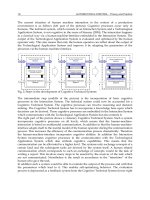
The bulk charge as
a
function of
Vd,
for different
V,,(>
Vth)
are shown
in Figure 7.5a while the gate charge as a function of
V,,

is
shown in
Figure 7.5b.
QI
=
Qs
+
QD
=
-
$Cox,
vgt
Weak
Inversion
Region.
Although mobile charge at the interface
is
small
when the device
is
in weak inversion, still these charges are important for
the simulation of switching behavior of a MOSFET. Further, in this region
bulk charge behaves differently as compared to the strong inversion
condition because it is now not screened from the channel.
In order to arrive at the expression for the terminal charges in the weak
inversion, we will assume that current transport occurs by diffusion only
as was the case while deriving the subthreshold drain current expression
[21].
Indeed this is
a

good approximation for low gate voltages. For higher
gate voltages
(>
Vth),
the diffusion current saturates and drift transport
becomes more and more important, as discussed in Chapter
6.
From
344
7 Dynamic Model
-2.01
I
I I
I
0
1
2
3
4
"h
0
Fig. 7.4 The normalized source and drain charges
Qs
and
QD,
respectively, as a function
of
V,,
for
different

V,,
in strong inversion. The normalization factor
is
total gate oxide
capacitance
Cox,
=
Cox
WL
Table 7.1.
nMOST
parameter ualues
used
.for Figures
7.6-7.9
Parameter Parameter
symbol Parameter description value Units
L
Effective channel length
50 Pm
W
Effective channel width 50 Pm
to*
Gate oxide thickness 150
A
A
Channel mobility
600
cm2/V.s
Flat band voltage

-
0.8
V
v,
h
Threshold voltage
0.6
V
N,
Substrate concentration 3
x
1OI6
cm-3
Eq.
(6.92)
the drain current (due to diffusion) at any point
y
along the
surface
is
given
by
(7.63)
which on integration yields
y=-
Vt(Qi
-
Qis)
(7.64)
where

V,
=
kT/q
is the thermal voltage and
Qis
is the mobile charge density
at the source end [cf.
Eq.
(6.95)].
At the drain end
Qi
=
Qid.
Id,
7.3
Long-Channel Charge Model
345
-0.55-
I
I
I
-
0.60
-
v,,=o
v
-
Fig.
3.5
3.0

-
-
-
I
I
I I
012345
Vgs
(V)
(a)
0.0
7.5
The normalized (a) gate charge
QG
as a function
of
V,,
for different
V,,,
(b)
bulk
charge
QB
as
a
function of
V,,
for different V,, in strong inversion
Let us first calculate the source and drain charge
QD

and
Qs,
respectively.
Application
of
Eqs. (7.63) and (7.64) with
Eq.
(7.49) results in
(7.65)
which
on
integration yields, after using
Eq.
(6.93) for
Ids,
QD
=
iWL(2Qid
+
Qis).
(7.66)
We can now relate charge densities
Qis
and
Qid
using Eq.
(6.95),
resulting
in the following equation for
QD

Q
D
-__
-
A
wLcox(q
-
l)vt
exp
(
vg~tvth)(2~pvds/vt
+
1)
(7.67)
where
q
=
(1
+
Cd/C,,)
[cf. Eq. (6.103)]. Similar procedures can be used for
calculating the source charge
Qs
and is found to be
Q
s
-_-
-
A
W~Co,(r1

-
1)V
exp
(vg$tvth)(e-vds/vt
+
2).
Note
that
when
V,,
=
0,
and
Vgs
=
T/rh,
we
have
QD
=
Qs
=
-
0.5C,,,(q
-
1)v.
From
Eq.
(7.67) it
is

evident that
Vd,
dependence
on
Qs
and
QD
is
rather
weak because for
Vds
greater than a few
V,,
the terms involving
vd,
become
negligible and we
find
Qs
=
20,.
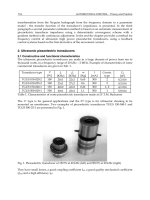
Figure 7.6 shows drain and source charges
346
7
Dynamic Model
v,,
(V)
Fig.
7.6
The normalized source and drain charges

Qs
and
QD,
respectively, as
a
function
of
V,,
for different
V,,,
in weak inversion
in weak inversion as a function of
Vd,
for two
V9,(
<
VJ.
The exponential
behavior is clearly visible as well as a weak drain bias dependence. Note
that the magnitudes of these charges are six orders of magnitude smaller
than those in strong inversion.
From the strong inversion Eq. (7.55) note that at
V,,
=
Ift,,,
QD
=
Qs
=
0,

while from weak inversion
Eq.
(7.67) we get small but finite values
of
Qs
and
QD.
This results in a discontinuity of these charges at the transition
from weak
to
the strong inversion. To avoid this discontinuiq, the weak
inversion charge must be added to the strong inversion charge. However,
this does complicates the charge equations. Although it results in a conti-
nuous
Qs
and
QD,
the corresponding capacitances at the transition point
will still be discontinuous (see Figures 7.8-7.10). In order to avoid the
discontinuity in the capacitance a smoothing function, such as Eq. (6.121)
used in the drain current modeling, can be used. Because
these charges
make only minor contributions to the total charges and they decrease
exponentially with decreasing
V,,,
we often assume
Qs
and
QD
to

be
zero in
weak inversion.
Since in weak inversion the bulk charge
QB
is virtually independent
of
the
source/drain voltage
Vd,,
we can use Eq.
(7.23)
for
QB,
which at the boundary
of
the strong inversion can be rewritten as
This equation is the same as to the first term in Eq. (7.60).
If
the channel charge is assumed zero
(QI
=
0)
in the subthreshold region,
the gate charge becomes equal to the bulk charge. Thus,
QB
=
-
Coxt~
Jm.

Qc
=
-
QB.
7.3
Long-Channel Charge Model
347
1
-2
-3
-4
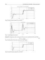
Fig.
7.7
The normalized plot
of
the charges
QG,Q,,Q,
and
Q,
associated with the gate,
bulk, drain and source terminals, respectively
Accumulation Region.
For the sake of completeness, we discuss charges in
the accumulation region of operation where
T/,b
<
T/fb.
In accumulation, a
thin layer of majority carriers are formed at the interface, thus forming a
parallel plate capacitor with the gate. In this case, the bulk charge

QB
is
simply written as
(7.68)
QB
=
-
co.xt(Vgs
+
vsb
-
Vfb).
Since there
is
no current
flow,
the gate charge is given by
QG
=
-
QB
=
coxt(vqs
+
vsb
-
vfb)*
(7.69)
Figure 7.7 shows charges
QG,

QB,
Qs
and
QD
associated with the gate, bulk,
source, and drain terminals, respectively, as a function of gate voltage
V,,
for
2
different drain voltages
V,,,
and fixed substrate bias
V,,
=
0
V.
The
parameters used for simulations are shown in Table 7.1. They are based
on the assumption that
Qs
=
QD
=
0
in inversion.
7.3.1
Capacitances
Using the expressions derived for various charges in different regions
of
device operation and the definition (7.40) we can now

find
the capacitances
associated with a
MOSFET.
The mathematics, though quite basic, is
however some times very lengthy. The final expression for 12 capacitances
are given
in
Appendix
F
using charges given in section 7.3. Figure 7.8
shows
348
7
Dynamic Model
h
U
(a)
00
8.0
(b)
Fig.
7.8
Measured and calculated capacitance (a) gate-to-drain C,, and
(b)
drain-to-gate
C,,
as a function
of
V,,

with
Vds
as
a
parameter
C,,
and
CDG
as a function of
Vqs
for different
Vds.
Continuous lines are
from the model [cf. Eqs. (7.70)], while dashed lines are measured data for a
long channel device
(W/L
=
100/100
pm,
V,,
=
0.8
V,
to,
=
305
A).
Remember
that measured capacitances also include gate overlap capacitances which
have been subtracted out in the data shown in this figure. The equations for

C,,
and
C,,
are obtained by differentiating
Q,
[Eq. (7.55a)l with respect
to
V,
(or
V,,)
and
Qc
[Eq.
(7.58)] with respect to
Vd
(or V,,), respectively, and
using
d'
and
&7
defined in Eq. (7.56), that
is,
0.5aI/,,
(7.70b)
These are the capacitances in the linear region. The corresponding capaci-
tances in the saturation region are obtained, either differentiating the
7.3
Long-Channel Charge
Model
349

saturation region charge [cf.
Eq.
(7.61)] or replacing
V,,
with
V,,,,
=
(
Vgt/a)
in
Eq.
(7.70),
resulting in the following expressions
(7.7 1 a)
(7.71b)
Figure 7.8 clearly shows the non-reciprocal nature of the capacitances. It
also shows that the model fits the data fairly well. Note that though the
transition from linear to saturation regions is smooth, the same is not the
case for transition from saturation to subthreshold regions due to our
assumption
of
QI
=
0
in the subthreshold region. Although continuity of
the capacitances is desirable, particularly in small signal analysis, the
discontinuity does not pose any convergence problem in
SPICE.
This is
because the capacitance value is multiplied by the voltage difference term

which vanishes as convergence is reached. Also note that
CD,
=
0
in the
saturation region. This is because of our assumption
of
the pinch-off
condition
(QI
=
0
at the drain end, which has resulted in
vd,,,
=
Vgt/a)
in
the charge expressions. For long channel devices, this indeed is observed
experimentally because pinch-off shields the channel from any further drain
voltage increase. It should be pointed out that
C,,
is most important
among the gate capacitances because its effect is multiplied by the voltage
gain between the drain and gate nodes due to the Miller effect.
Figure 7.9 shows
C,,
and
C,,
as a function of
Vgs

for different
Vds.
Again,
continuous lines are from the model [cf.
Eq.
(7.72)], while dashed lines are
measured data for a long channel device
(W/L
=
100/100pm,
vth
=
0.8
V,
to,
=
305
A).
The
C,,
and
C,,
are obtained by differentiating
Q,
[Eq.
(7.58)]
with respect to
V,
and
Q,

[Eq.
(7.55b)l with respect to
Vg
(or
V,,),
respectively,
and using
Se
and
B
defined in
Eq.
(7.56),
that is,
In the saturation region we have
(7.72b)
(7.73a)
c,,
=
+
cox,.
(7.7
3
b)
Again the non-reciprocal nature of the capacitance is self evident.
350
7
Dynamic Model
a
v

0
0.0
t
0.0
Fig.
7.9
Measured and calculated capacitance (a) gate-to-source
C,,
and
(b)
source-to-gate
C,,
as a function
of
V,,
with
V,,
as a parameter
The gate-to-bulk capacitance
C,,
is shown in Figure
7.10
as
a
function of
V,,
for different
Vds.
The model equation (continuous line) for
C,,

is given
in Appendix
F.
Although this capacitance is much smaller in strong
inversion,
it
is the main capacitance in weak inversion and accumulation.
Figure 7.11 shows plots
of
nine internodal capacitances as a function
of
Vds.
The capacitances are normalized to the total gate capacitance
Cox,(
=
WLC,,).
For the sake
of
clarity, these capacitances are plotted at
one bias,
V,,
=
3
V
and
V,,
=
0
V.
Note from this figure that the capacitances

C,,
and
C,,
are negative. This shows that
MOS
capacitors are not only
non-reciprocal but are negative
too.
This negative capacitance
could
be
explained as follows. Consider
C,,
when the device
is
biased with say
Vd,
=
1
V.
This capacitance is the result of a small change in the drain charge
due to change in the source voltage keeping all other voltages constants.
From Eq.
(7.50)
it is evident that a small increase in the source voltage will
result in an increase in the inversion charge
Qr,
i.e., the total number
of
mobile electrons in the channel will increase. Since the device is biased

7.3
Long-Channel Charge Model
351
GATE
VOLTAGE,
Vq5
(V)
Fig. 7.10 Measured and calculated gate-to-bulk capacitance
C,,
as
a
function
of
V,,
with
Vds
as
parameter
DRAIN
VOLTAGE,
V,,
(V)
Fig. 7.11 Normalized plots
of
9
internodal capacitances versus drain voltage at
Vgs
=
3.0V
and

V,,
=
0
V
symmetrically, some of this increase in charge will be supplied by the drain,
and if the drain supplies positive charge when the source voltage increases,
a negative capacitance is observed by definition [cf. Eq.
(7.40)].
Also note from Figure
7.1
1
that
C,,
#
C,,
at
Vd,
=
0
V,
although by
symmetry they should be equal. The reason for this discrepancy is the value
of
6
(in
a)
used for the square root approximation (cf. section 6.4.3).
By
substituting
V&=O

in
Eqs. (F.3a) and (F.3b) (Appendix
F)
for
C,,
and
352
0.61
I I
I
I
7
Dynamic Model
Fig. 7.12 Normalized plot of the drain-to-source and source-to-drain capacitance
C,,
and
C,,,
respectively,
for
two different expressions for
6
function. Solid lines are based on
6
value
from
Eq.
(6.73), while dashed lines correspond
to
6
given

by
Eq.
(6.70)
C,,,
respectively, we get
1
CB,
=
cox*[
av,,
-
OS(a
-
1)
(7.74)
CB,
=
0.5CoX,(a
-
1).
At
V,,
=
OV,
we get
CB,
=
CB,
=
0.5~8

provided we assume
6
=
0.51
Jm
[cf. Eq. (6.71)] in the bulk charge approximation. For the drain
current modeling it is common practise to slightly modify the value for
6
to obtain better fits in the drain current versus drain voltage plot (cf. section
6.5). However, this will lead to a small discontinuity in the capacitance.
This difference is more evident when we plot drain and source capacitances
C,,
and
C,,,
respectively, as a function of
Vds.
This is shown in Figure 7.12,
where dashed lines assume
Eq.
(6.71) for
6,
while continuous lines assume
Eq.
(6.73) for
6.
The situations in which these discrepancies arise have
comparatively small capacitances, therefore, it is not the cause
of
any
significant error in circuit simulation when all capacitances at a node point

are added together.
7.4
Short-Channel Charge
Model
In the long channel model discussed in the previous section we have
neglected velocity saturation, channel length modulation and series resis-
tance, as these effects are important only for short-channel devices (cf.
7.4
Short-Channel Charge
Model
353
section 6.7).
As
in the case of drain current calculations, we need to take
these effects into account while calculating charges for short channel
devices
[14,15], 1181,
[25]. Indeed the final charge equations become more
complex.
Often for simulating short-channel capacitances, the long channel charge
model has been used by modifying the body factor
a
[7], [12]. Thus, in
the model proposed by Yang et al. [7], the
a
term in the long channel
charge expressions (cf. section 7.3) is replaced by
a,
=
a1

+
a2(
Vgs
-
Vth)
where
a1
and
a2
are short-channel fitting parameters [7]. They
also
assume
QD
=
0
in the saturation region due to the fact that the channel is isolated
from the drain. In the BSIM model (SPICE Level
4
model) 1121, the
a
term in the long channel charge expressions is replaced by
a,
such that
a,
=
a(1
+
O(V,,
-
Vth)).

In this case
a,
is
no longer
a
simple body factor
term, but is now effective gate voltage dependent, similar to the Yang et al.
[7]
model. However, to arrive at more accurate charge and capacitance
expressions for short-channel devices, one must take into account short-
channel effects such as carrier velocity saturation, channel length modu-
lation and source/drain series resistance. We will now show how to include
these effects
in
the charge equations, which in turn will be used for the
derivation of short-channel capacitances.
Recall that
I,,
for short-channel devices in the linear region is given by
(cf. section 6.7.1)
Replacing
by
by
(dV/dy)
and rearranging we get
Integrating this equation yields
(7.75)
(7.76)
(7.77)
Substituting

y
=
L
and
V
=
V,,
(at the drain end) in the above equation
permits solution for
I,,.
Remember that
Q,
=
usat/ps
[cf.
Eq.
(6.158)], where
p,
depends upon S/D resistance.
Let us first calculate
QD
and
Qs.
Following the same procedure as was
used for long channel devices (cf. section 7.3), we get the following expres-
sions
for the source and drain charges in the linear region of device
operation
(7.78a)
(7.78

b)
QD
=
-
C,,,,[$V,,
-
faVds
-
.d"&7']
Qs
=
-
Cox,
[i
vgt
-
iaVds
+
d'(
1
+
a')]
354
7
Dynamic
Model
where
(7.79a)
(7.79b)
and

d
and
98
itself are given by Eqs. (7.56a) and (7.56b), respectively.
Comparing the above equations with long channel
Qs
and
QD
equations
(7.55) we see that the two equations have the same form, except that the
auxiliary functions
d‘
and
B‘
now contain
a
velocity saturation factor.
For the long-channel case, when the product
Lb,
is very large, Eq. (7.78)
reduces to
Eq.
(7.55)
as
is expected.
The remaining charges can also be derived in a similar way as for long
channel devices. Thus, the gate charge for short-channel devices can be
derived as
(7.80)
Substituting

Qi
and
Q,
from Eq. (7.50) and (7.52) and carrying out the
integration we get, after lengthy algebra, the following equation for
QG
in
the linear region
Qc
=
Coxt[
Vgs
-
Vfb
-
24f
-,0.5Vds
+
-d’
.
(7.81)
Here again, for long channel devices the above equation reduces to Eq.
(7.58). Similarly one can derive the bulk charge expression
as
a
l1
(7.82)
(7.82a)
and
9

is given by
Eq.
(7.60a).
Recall that while deriving the long-channel charges in saturation, we
simply
replaced the drain voltage
V,,
in the linear region charge expressions by the
drain saturation voltage
V,,,,.
However, for short-channel devices, where
velocity saturation and channel length modulation
(CLM)
become impor-
tant, the charges in saturation consists of two components. One
is
the
charge near the source region (region
I
in Figure 7.13) where the gradual
channel approximation
(GCA)
can be applied and the other is charge near
the drain end (region
I1
in Figure 7.13) where carrier velocity saturates.
7.4
Short-Channel Charge Model
0.0
355

I
I
1
v,,
=
0
VJ
Region
I
Region
11
Fig.
7.13
Two-section model
for
calculating short-channel capacitance in saturation
-2.0
Thus, in general
Qj(saturation)
=
Qjl
(linear)lVds+Vdsat
+
Qj2(over the distance
Id)
where
1,
is the
CLM
region near the drain end (cf. section

6.7.3).
Assuming
that over the distance
1,
carriers travel with saturated velocity, we can write
Qj2
as
Ids
d
Q.
=-l
J2
vsat
This two section model does create a discontinuity in the capacitances
from linear to saturation regions, similar to the case
of
drain current
modeling. Therefore, often Qj2 is ignored for short-channel modeling, unless
one can
use
smoothing functions such as discussed in section
6.7.4.
The effect
of
including velocity saturation in the charge expressions
is
a
reduction in the amount of charge from its long channel value, which
intuitively makes sense, because carriers are velocity saturated. This is
shown in Figure

7.14
for
Qs
and
QD
with and without velocity saturation,
_
No
Velocity
Saturation
I
I I
I
1
o*
2
d

-0.3
-
QD
,,
,,(,,,,,,,
,,,,,,,
,,,,(,,
,, (


,

'
Qs
W
- -
/I-==
___________________
-0.8
-
-1.0
-
Fig. 7.14 The normalized source and drain charges, Qs and Qd, respectively, as a function
of Vds for different Vgs, with and without velocity saturation
356
7
Dynamic
Model
respectively, and assuming
1,
=
0.
Although the effect of
S/D
resistance
is
taken into account it is possible to include its effect externally
[18].
In the weak inversion,
QI,
hence
Q,

and
Q,,
is assumed zero, similar to
the long channel case. This means that
Q,
=
-
Q,
in the weak inversion.
The bulk charge
QB
for short channel devices is still given by
Eq.
(7.23),
but with the long channel body factor
y
replaced by the effective
y,
which
takes into account the reduction in the bulk charge density due to short-
channel and narrow-width effects as discussed in Chapter
5.
7.4.1
Capacitances
Once charges are known, the corresponding capacitances can easily be
calculated using the same procedure as discussed earlier for the long channel
case. The mathematics is basic, but lengthy. We will not derive the final
expressions for the capacitances. Instead, here we will show some experi-
mental data for short channel devices and compare their behavior with
long channel devices.

It should be pointed out that unlike the long channel capacitances, the
short channel capacitance measurement is not a trivial task. This is because
of
very small values of the capacitances involved (in the
aF
range); the
details of measurements are discussed in section 9.7. Moreover, for short
channel devices, due to the large steady-state current
(Ids)
it is very difficult
to separate out small transient currents due to the capacitances associated
with the source and drain terminals. For this reason, only short channel
capacitances that have been measured and reported todate are the gate
capacitances
C,,,
C,, and
C,,.
Figure 7.15 shows measured
C,,
(normalized
to
C,,,) for an n-channel
LDD
MOSFET
with
W/L
=
50/0.65
and
to,

=
105
A.
The measured data for long channel device
W/L
=
50/50 is also
shown for comparison. These are devices fabricated using 0.75 pm CMOS
technology with
AL
=
0.25
pm. Note that in the linear region the short
channel
C,, is larger than the long channel
C,,,
which is more evident at
higher
Vds.
This is due to the velocity saturation effect, which causes
Qr
to
be proportional to
I,,,
and hence modulating
V,
has an additional effect
on
QI
through change in

Ids.
In the saturation region, the short channel
C,,
decreases with increasing
V,,
due to the
CLM
effect, while the long
channel
C,,
is independent of
V,,
in saturation. Unlike constant
C,,
in
the cut-off region
(V,,
<
Vth)
for long channel devices, the short channel
C,, increases due to channel side fringing field effect at the source end.
The short channel
C,,
is shown in Figure7.16. For comparison, long
channel
C,,
is also shown. Here again changes in short channel
CGD
behavior can be explained by velocity saturation, channel length modulation
and channel fringing field effect. Figure 7.17 shows

C,,
as a function
of
7.4
Short-Channel Charge Model
0.8
0.6
0.4
0.2
0.oi
351
I
I
1
I
v,=ov
to=
=
105
A
-
-
-
_____
WL=50/50@m)
-
-
WL
=
50/0.65

@m)
I
,'
*.I'
__
I I
I
Fig.
7.15
Measured short and long channel gate-to-source capacitance
C,,
of
V,,
with
V,,
as
a parameter
v,,=ov
t,
=
105
A
.___
W/L
=
50/50
@m)
-
WL
=

50/0.65
@m)
0.6
v,,=ov
as a function
Fig.
7.16
Measured short and long chemical gate-to-drain capacitance
C,,
as a function
of
V',,
with
V,,
as a parameter
gate voltage. Note that higher
V,,
results in smaller
CGB
in
the cut-off
region.
As
V,,
increases, more
bulk
charge will be associated with the drain
junction which results
in
less bulk charge available to modulate the gate

charge. In the strong inversion region, the short channel
C,,
is much
smaller than the long channel
C,,
for the same reason.
In
all cases the
358
7
Dynamic Model
I
0
u,
rn
V
V
I,,
=
105
I
-"
0.2
A
L
4.0
-2.0
0.0
2.0
4.0

"gs
(v)
Fig.
7.17
Measured short and long channel gate-to-source capacitance
CGB
as a function
of
V,,
with
V,,
as a parameter
short channel gate capacitances varies more gradually from one region to
the other as compared to the long channel device.
The measured capacitances shown in Figures 7.15-7.17 includes the overlap
capacitances and as such, they are not intrinsic capacitances. Note from
Figure
7.16,
the overlap capacitance (measured capacitance in accumulation)
is drain and gate bias dependent. This is true particularly
for
short channel
LDD
devices
[18].
However, no such bias dependent overlap is generally
observed in short-channel conventional source/drain junctions. The bias
dependence of the overlap capacitance is due to the modulation
of
the

,/
I
,
'.
I
ACCUMULATION
Fig.
7.18
Different components constituting MOSFET overlap capacitance in a LDD
device. (After Smedes
[18])
7.5
Limitations of the Quasi-Static Model
359
lightly doped n-region. It has been modeled using parallel combination of
three components associated with the bottom, the sidewall and the
top
of
the gate
Cbo,,
Cside
and
Ctop,
respectively, and is given by (see Figure
7.18)
Cl
81
with
(7.83)
(7.84)

where
1,”
is the geometrical overlap.
7.5
Limitations
of
the Quasi-Static Model
The MOSFET charge and capacitance models discussed
so
far are based
on the quasi-static assumption; that is, terminal voltages vary sufficiently
slowly
so
that the stored charge
(Qc, Qe, Qs
and
QD)
can follow voltage
variations. It has been found that for much of the digital circuit work the
quasi-static model gives acceptable accuracy if the rise time
t,
of the
waveforms involved is such that
[
11
t,
<
15z,
(7.85)
where

zt
is the transit time associated with the
DC
operation of the device.
It
is
defined as the average time the inversion carriers take to travel the
length of the channel, that is,
Using
Eq.
(7.62) for
QI
and
Eq.
(6.84) for
I,,
in saturation, we get7
4
L2
-a
-
-
4
L2
3
PL,(l/gS
-
Vth)
3
Vdsa,

z,
=-a
(7.86)
(7.87)
This shows that transit time
is
proportional to L2. The shorter the
L,
the
smaller the transit time, and thus the higher the speed. If the carriers are
velocity saturated then Eq.
(7.87)
becomes invalid and one needs to use
Qr
and
Id,
equations discussed in section 6.7. However,
a
simple estimate for
z
can still be made assuming carriers are moving from source to drain with
In the linear region, under the condition of V,,
=
0,
we have
QI
=
WLC,,(
Vgs
~

Vt,J
and
therefore
T
N
L2/Vd,.
3
60
7
Dynamic
Model
their scatter limited saturation velocity
usat
for the whole length of the
channel rather than only part of the channel. Since carriers cannot move
faster than
us,,,
the time required for the drain current
to
respond to the
changes in the gate voltage is simply
usa,/L.
Thus, in general
L
z,
>

"sat
(7.88)
Assuming

L=
1
pm and
usat
=
lo7
cm/s, the transit time is around
10
ps.
For a typical ring oscillator circuit with
1
pm channel length
MOSFETs,
the measured delay is of the order of
10
ns. This shows that switching is
limited by the parasitic capacitances rather than the time required for the
charge redistribution within the transistor itself. Thus, quasi-static operation
is good enough for most of the cases.
It should be pointed out that Eq. (7.85) is only a rough rule of thumb and
often, due to the significant extrinsic parasitic capacitances, this rule is not
restrictive. In fact the parasitic capacitances can mask the error due
to
the
quasi-static assumption. However,
if
parasitic capacitances are indeed low
and input changes in the waveforms are too fast then the quasi-static model
will break down.
In such situations, one way to extend the quasi-static model

is to consider the device as a connection of several sections, each section
being short enough to be modeled quasi-statistically
[l].
However, more
correctly, one needs to include time dependence in the basic charge
equations. The resulting analysis is called non-quasistatic
(NQS) analysis.
The
NQS
is not covered here and interested readers are referred
to
the
references cited
[l],
[20], [30]-[34].
7.6
Small-Signal Model Parameters
In this section we will discuss MOSFET small-signal parameters discussed
in section 3.2.1, namely
g,,
gds
and
gmbs.
These parameters are required for
the small-signal analysis. In addition they are also required for linearizing
nonlinear drain current models. The output conductance
gds
and trans-
conductance
g,

are important parameters in analog circuit design. As
was pointed
out
earlier, these parameters can easily be derived from
the device drain current model discussed in Chapter 6. This means that
Id,
equations must be differentiable with respect to all terminal voltages. This
is also important for SPICE convergence process since discontinuous
derivatives can result in nonconvergence of the solution.
For the sake of simplicity, let us consider the
Id,
equation discussed in
section 6.4.4. Application of definition (3.1 1)
to
the drain current
Eq.
(6.47)
and assuming
,us
is constant independent of
Vgs
(to first order), yields
ctvd,)
(linear region,
Vd,
I
V,,,,)
(saturation region,
V,,
>

V,,,,).
(7.89)