MOSFET MODELING FOR VLSI SIMULATION - Theory and Practice Episode 14 potx

496
9 Data Acquisition and Model Parameter Measurements
1321
S.
H.
Lin and J. Reuter, ‘The complete doping profile using MOS CV technique’,
Solid-state Electron., 26, pp. 343-351 (1983).
1331
G.
Baccarani,
H.
Rudan,
G.
Spaini,
H.
Maes, W.
V.
Ander Vorst, and R. Van
Overstraeten, ‘Interpretation of C-V measurements for determining the doping profile
in semiconductors’, Solid-state Electron., 23, pp. 65-7
I
(1980).
1341 C. P. Wu, E. C. Douglas, and C. W. Mueller, ‘Limitations
of
the C-V technique for
ion-implanted profiles’, IEEE Trans. Electron Devices,
ED-22,
pp. 319 329 (1975).
[35] B. J. Gordon, ‘On-line capacitance-voltage doping profile measurement’, IEEE
Trans. Electron Devices, ED-27, pp. 2268-2272 (1980).
[36] K. Lehovec, ‘C-V profiling of steep dopant distribution’, Solid-State Electron., 27,

[37]
I.
G.
McGillivray,
J.
M. Robertson, and A.
J.
Walton, ‘Improved measurement
of
doping profile in silicon using CV techniques’, IEEE Trans. Electron Devices, ED-35,
pp. 174-179 (1988).
1381 K. Iniewski and C. A. T. Salama, ‘A new approach to CV profiling with sub-debye-
length resolution,’ Solid-state Electron., 34, pp. 309-3 14 (1991).
[39]
G.
Lubberts, ‘Rapid determination of semiconductor doping and flatband voltage
in large MOSFETs’,
J.
Appl. Phys., 48, pp. 5355-5356 (1977).
1401 J. A. Wikstrom and C.
R.
Viswanathan, ‘A direct depletion capacitance measurement
technique to determine the doping profile under the gate
of
a
MOSFET’, IEEE Trans.
Electron Devices,
ED-34,
pp, 2217-2219 (1987).
[41] M. Shannon, ‘DC measurement of the space charge capacitance and impurity profile

beneath the gate of an MOST’, Solid-state Electron., 14, pp. 1099-1 106 (1971).
[42] M.
G.
Buchler, ‘Dopant profiles determined from enhancement-mode MOSFET DC
measurements’, Appl. Phys. Lett., 31, pp. 848-850 (1977).
1431 M.
H.
Chi and C. M.
Hu,
‘Errors in threshold-voltage measurements of MOS
transistors for dopant-profile determinations’, Solid-state Electron., 24, pp. 313-316
(1981).
1441
G.
P.
Carver, ‘Influence of short-channel effects on dopant profiles obtained from the
DC MOSFET profile method’, IEEE Trans. Electron Devices, ED-30, pp. 948-953
(1983).
[45] N. Kasai,
N.
Endo,
A.
Ishitani, and Y. Kurogi, ‘Impurity profile measurement using
VT
-
Vss
characteristics,’ NEC Res.
&
Develop., 74, pp. 109-114 (1984).
1461

K.
lniewski and A. Jakubowski,
‘A
new method for the determination of channel
depth and doping profile in buried-channel MOS transistors’, Solid-state Electron.,
[47] D. W. Feldbaumer and D. K. Schroder, ‘MOSFET doping profiling’, IEEE Trans.
Electron Devices, ED-18, pp. 135-139 (1991).
[48]
H.
G.
Lee,
S.
Y. Oh, and
G.
Fuller, ‘A Simple and accurate method to measure the
threshold voltage
of
an enhancement-mode MOSFET’, IEEE Trans. Electron Dev.,
[49]
H.
S.
Wong, M.
H.
White,
T.
J. Krutsick, and R. V. Booth, ‘Modeling of transconduc-
tance degradation and extraction of threshold voltage in thin oxide MOSFETs’,
Solid-state Electron., 30, pp. 953-968 (1987).
[SO]
R.

V.
Booth,
H.
S.
Wong, M.
H.
White, and T.
J.
Krutsick, ‘The effect
of
channel
implants
on
MOS
transistor characterization’, IEEE Trans. Electron Devices, ED-34,
1511
S.
Jain, ‘Measurement
of
threshold voltage and channel length
of
submicron
MOSFETs’, Proc. IEE, Pt.
I,
135, pp. 162-164 (1988).
[52] M. J. Deen and
Z.
X.
Yan,
‘A

new method for measuring the threshold voltage of
small-geometry MOSFETs from subthreshold conduction’, Solid-state Electron., 33,
pp. 1097-1
I05
(1984).
31, pp. 1259-1264 (1988).
ED-29,
pp. 346-348 (1982).
pp. 2501 -2508
(1
987).
pp. 503-511 (1990).
References 497
[53] C.
G.
Sodini,
T.
W. Ekstedt, and J. L. Moll, ‘Charge accumulation and mobility in
thin dielectric
MOS
transistors’, Solid-state Electron., 25, pp. 833-841 (1982).
[54]
N.
D.
Arora and
G.
Sh. Gildenblat,
‘A
semi-empirical model of the MOSFET
inversion layer mobility for low-temperature operation’, IEEE Trans. Electron

Devices, ED-34, pp. 89-93 (1987).
[55]
J.
Kooman, ‘Investigation
of
MOST
channel conductance in week inversion’,
Solid-State Electron., 16, pp. 801-810 (1973).
[56]
M.
S.
Liang,
J.
Y. Choi, P. K.
KO,
and C.
M.
Hu, ‘Inversion-layer capacitance and
mobility
of
very thin gate-oxide MOSFETs’, IEEE Trans. Electron Devices, ED-33,
1571 P M.
D.
Chow and K L. Wang, ‘A new AC technique for accurate determination
of
channel charge and mobility in very thin gate MOSFETs’, IEEE Trans. Electron
Devices, ED-33, pp. 1299-1 304 (1986).
[58]
G.
Sh. Gildenblat, C L. Huang, and N. D. Arora, ‘Split C-V measurements of low

temperature MOSFET inversion layer mobility,’ Cryogenics, 29, pp. 1163-1 166
(1989)
[58a] C. L. Huang, J. Faricelli, and N. D. Arora,
‘A
new technique for measuring MOSFET
inversion layer mobility’, IEEE Trans. Electron Devices, ED-40, pp.
11
34-1 139
(1993).
1591
A.
Hairapetian, D. Gitlin, and C.
R.
Viswanathan, ‘Low-temperature mobility
measurements
on
CMOS devices’, IEEE Trans. Electron Devices, ED-36, pp.
1448-1445 (1989).
[60]
K.
Terada and H. Muta,
‘A
new method to determine effective MOSFET channel
length’, Japanese
J.
Appl. Phys., 18, pp. 953-959 (1979).
[61]
J.
G.
J.

Chern,
P.
Chang,
R.
F. Motta, and N. Godinho,
‘A
new method to determine
MOSFET channel length’, IEEE Electron Device Lett., EDL-I, pp. 170-173 (1980).
1621
S.
E. Laux, ‘Accuracy of an effective channel length/external resistance extraction
algorithm for MOSFETs’, ED-31, pp. 1245-1251 (1984).
[631
J.
Scarpulla and J. P. Krusius, ‘Improved statistical method for extraction
of
MOSFET effective channel length and resistance’, IEEE Trans. Electron Devices,
1641 B.
J.
Sheu, C. Hu,
P.
K. KO, and F C. Hsu, ‘Source-and-drain series resistance
of
LDD MOSFETs’, IEEE Electron Device Lett., EDL-5,
pp.
365-367 (1984).
[65]
K.
K.
Ng and

J.
R.
Brews, ‘Measuring the effective channel length of MOSFETs’,
IEEE Circuits and Devices Magazine, 6, pp. 33-38, Nov. 1990.
C661
M.
R.
Wordeman, J. Y C. Sun, and
S.
E. Laux, ‘Geometry effects in MOSFET
channel length extraction algorithms’,
IEEE
Electron Device Lett., EDL-6, pp. 186-
188 (1985).
1671 J. Y C. Sun,
M.
R. Wordeman, and
S.
E. Laux, ‘On the accuracy
of
channel length
pp. 409-413 (1986).
ED-34,
pp.
1354-1359 (1987).
characterization of LDD MOSFETs’, IEEE Trans. Electron Devices, ED-33, pp,
1556-1562 (1986).
.I
[68] D.
J.

Mountain, ‘Application
of
electrical effective channel length and external
resistance measurement techniques to a submicrorneter
CMOS
process’, IEEE Trans.
Electron Devices, ED-36, pp. 2499-2505 (1989).
[69] G.
J.
Hu, C. Chang, and
Y.
T. Chia, ‘Gate-voltage-dependent effective channel length
and series resistance of LDD MOSFETs’, IEEE Trans. Electron Devices, ED-34,
[70] J. Ida, A. Kita, and F. Ichikawa, ‘Accurate characterization
of
gate-N- overlapped
LDD with the new Leff extraction method, IEEE IEDM,
Tech.
Dig.,
pp. 219-222
(
1990).
1711
K.
L. Peng, and M. A. Afromowitz, ‘An improved method to determine MOSFET
channel length’, IEEE Electron Device Lett., EDL-3, pp. 360-362 (1982).
pp. 2469-2475 (1987).
498
9 Data Acquisition and Model Parameter Measurements
[72] J. Whitfield, ‘A modification on an improved method to determine MOSFET channel

length’, IEEE Electron Device Lett., EDL-6, pp. 109-110 (1985).
[73]
J.
H.
Satter, ‘Effective length and width
of
MOSFETs determined with three
transistors’, Solid-state Electron., 30, pp. 821-828 (1987).
[74] D. Takacs, W. Muller, and
U.
Schwabe, ‘Electrical measurement
of
feature sizes in
MOS Si-gate VLSI technology,’ IEEE Trans. Electron Devices, ED-27, pp. 1368-
1373 (1980).
[75] K. L. Peng,
S.
Y.
Oh, M. A. Afromowitz, and
J.
L. Moll, ‘Basic parameter measurement
and channel broadening effect in the submicron MOSFET,’ IEEE Electron Device
Lett., EDL-5, pp. 473-475 (1984).
[76] C. Hao,
B.
Cabon-Till,
S.
Cristoloveanu, and G. Ghibaudo, ‘Experimental determina-
tion of short-channel MOSFET parameters’, Solid-state Electron., 28, pp. 1025- 1030
(1985).

[77] L. Chang and
J.
Berg,
‘A
derivative method to determine a MOSFETs effective
channel length and width electrically’, IEEE Electron Device Lett., EDL-7, pp. 229-
231 (1986).
1781 D. Takacs. W. Muller. and
U.
Schwabe. ‘Electrical measurement
of
feature sizes in
L-
MOS Si-gate VLSI technology’, IEEE Trans. Electron Devices, ED-27, pp. 1368-1373
(1980).
1791
P.
P.
Such and
R.
L. Johnston, ‘Experimental derivation
of
the source and drain
resistance
of
MOS transistors’, IEEE Trans. Electron Devices, ED-27, pp. 1556-
1162 (1980).
[SO]
F.
H.

De La Moneda,
H.
N. Kotecha, and M. Shatzkes, ‘Measurement
of
MOSFET
constant’, IEEE Electron Device Lett., EDL-3, pp. 10-12 (1982).
[81]
G.
Krieger,
R.
Sikora,
P. P.
Cuevas, and M. N. Misheloff, ‘Moderately doped
NMOS(M-LDD)-hot electron and current drive optimization’, IEEE Trans. Electron
Devices, ED-38, pp. 121-127 (1991).
[82] G. Ghibaudo, ‘New method
for
the extraction
of
MOSFET parameters’, Electronic
Letters, 24, pp. 543-545, 28th April 1988.
[83]
Y.
R.
Ma and K. L. Wang, ‘A new method to electrically determine effective MOSFET
channel width’, IEEE Trans. Electron Devices, ED-29, pp. 1825-1827 (1982).
[S4]
B.
J.
Sheu and

P.
K.
KO,
‘A
simple method to determine channel widths for
conventional and LDD MOSFETs’, IEEE Electron Device Lett., EDL-5, pp. 485-486
(1984).
[85]
N.
D.
Arora, L.
A.
Bair,
and
L.
M. Richardson,
‘A
new method to determine the
MOSFET effective channel width’, IEEE Trans. Electron Devices, ED-37, pp. 81 1-814
(1990).
[86]
P.
Vitanov,
U.
Schwabe, and
I.
Eisele, ‘Electrical characterization
of
feature sizes and
parasitic capacitances using a single structure’, IEEE Trans. Electron Devices, ED-31,

[87] E. J. Korma,
K.
Visser,
J.
Snijder, and
J.
F. Verwey, ‘Fast determination
of
the effective
channel length and the gate oxide thickness in polycrystalline silicon MOSFETs’,
IEEE Electron Device Lett., EDL-5, pp. 368-370 (1984).
[88]
B.
J.
Sheu and
P.
K.
KO,
‘A
capacitance method to determine channel lengths
for
conventional and LDD MOSFETs’, IEEE Electron Device Lett., EDL-5, pp. 491-493
(1984).
[SY]
C.
T.
Yao,
I.
A.
Mack, and

H.
C. Lin, ‘Accuracy
of
effective channel-length extraction
using the capacitance method’, IEEE Electron Device Lett., EDL-7, pp. 268-270
(1986).
[90]
J.
Scarpulla, T. C. Mele, and
J.
P.
Krusius, ‘Accurate criterion
for
MOSFET effective
gate length extraction using the capacitance method, IEEE IEDM,
Tech.
Dig.,
pp.
pp. 96-100 (1984).
722-725 (1987).
References 499
[91] N. D. Arora, D. A. Bell, and L. A. Bair, ‘An accurate method
of
determining MOSFET
gate overlap capacitance’, Solid-state Electron., 35, pp. 1817-1822 (1992).
[92] P. Antognetti, C. Lombardi, and D. Antoniadis, ‘Use
of
process and 2-D MOS
simulation in the study of doping profile influence on S/D resistance in short channel
MOSFETs’, IEDM,

Tech. Digest,
pp. 574-577 (1981).
[93] M. H. Seavey, ‘Source and drain resistance determination for MOSFETs’, IEEE
Electron Device Lett., EDL-5, pp. 479-481 (1984).
[94]
K. K.
Ng and W. T. Lynch, ‘Analysis
of
the gate-voltage dependent series resistance
of
MOSFETs’, IEEE Trans. Electron Devices, ED-33, pp. 965-972 (1986).
[95]
A.
Vladimirescu and
S.
Liu, ‘The simulation of
MOS
integrated circuits using
SPICET, Memorandum
No.
UCB/ERL M80/7, Electronics Research Laboratory,
University of California, Berkeley, October 1980.
[96] T.
Y.
Chan,
P.
K.
KO,
and C. Hu, ‘A simple method to characterize substrate current in
MOSFETs’, IEEE Trans. Electron Device Lett., EDL-5, pp. 505-507 (1984).

[97] D. Lau,
G.
Gildenblat,
C.
G.
Sodini, and D. E. Nelsen, ‘Low temperature substrate
current characterization
of
n-channel MOSFETs’, IEEE-IEDM85,
Technical
Digest,
pp. 565-568 (1985).
[98]
R.
V.
H.
Booth and M.
H.
White, ‘An experimental method for determination
of
the
saturation point
of
a MOSFET’, IEEE Trans. Electron Devices, ED-31, pp. 247-251
(1984).
1991 W. Y. Jang,
C.
Y. Wu, and H.
J.
Wu,

‘A
new experimental method to determine the
saturation voltage
of
a small-geometry MOSFET’, Solid-state Electronic, 31, pp.
[loo]
H.
Iwai and
S.
Kohyama, ‘On-chip capacitance measurement circuits in VLSI
structures’, IEEE Trans. Electron Devices, ED-29, pp. 1622-1626 (1982).
[loll
J.
Oristian, H. Iwai, J. Walker, and R. Dutton, ‘Small geometry MOS transistor
capacitance measurements method using simple on-chip circuit’, IEEE Electron
Device Lett., EDL-5, pp. 395-397 (1984).
[lo21
H.
Iwai,
J.
Oristian,
J.
Walker, and
R.
Dutton,
‘A
scaleable technique for the
measurements
of
intrinsic MOS capacitance with atto-Farad range’, IEEE Trans.

Electron Devices, ED-32, pp. 344-356 (1985).
[lo31 J.
J.
Paulous, ‘Measurement
of
minimum-geometry MOS transistor capacitances’,
[lo41
C.
T. Yao and
H.
C. Lin, ‘Comments on small geometry
MOS
transistor capacitance
measurements method using simple on-chip circuit’, IEEE Electron Device Lett.,
[lo51
J.
Oristian,
H.
Iwai,
J.
Walker, and R. Dutton, ‘A reply to comments on “small
geometry
MOS
transistor capacitance measurements method using simple on-chip
circuit”’, IEEE Electron Device Lett., EDL-6, pp. 64-67 (1985).
[lo61
J.
J.
Paulos and D.
A.

Antoniadis, ‘Measurement
of
minimum geometry MOS
transistor capacitances’, IEEE Trans. Electron Devices, ED-32, pp. 357-363 (1985).
Also
see
J. J.
Paulos, ‘Measurement and modeling
of
small geometry MOS transistor
capacitance’,
Ph.D
thesis,
Massachusetts Institute
of
Technology, Cambridge, 1984.
[lo71 M. Furukawa, H. Hatano, and
K.
Hanihara,, ‘Precision measurement technique
of
integrated MOS capacitor mismatching using a simple on-chip circuit’, IEEE Trans.
Electron Devices, ED-33, pp. 938-944 (1986).
[lo81
K.
C.
K.
Weng and
P.
Yang,
‘A

direct measurement technique
for
small geometry
MOS transistor capacitances’, IEEE Electron Device Lett., EDL-6, pp. 40-42
(1985).
[lo91
H.
Ishiuchi,
Y.
Matsumoto,
S.
Sawada, and
0.
Ozawa, ‘Measurement
of
intrinsic
capacitance
of
lightly doped drain (LDD) MOSFET’s’, IEEE Trans. Electron Devices,
1421-1431 (1988).
ED-32, pp. 357-363 (1985).
EDL-6, p. 63 (1985).
ED-32, pp. 2238-2242 (1985).
so0
9
Data Acquisition and Model Parameter Measurements
[l lo]
Y.
T.
Yeow, ‘Measurement and numerical modeling

of
short channel MOSFET gate
capacitances’, IEEE Trans. Electron Devices, ED-35, pp.
2510-2519 (1987).
[lll]
B.
J.
Sheu and
P.
K. KO, ‘Measurement and modeling
of
short-channel
MOS
transistor gate capacitances’,
IEEE
J.
Solid-state Circuits, SC-22, pp.
464-472
(1
987).
[I
121
P. Leclaire, ‘High resolution intrinsic MOS capacitance measurement system’,
EESDERC
1987, Tech. Digest.,
pp.
699-702 (1987).
[I
131
C.

T. Yao, ‘Measurement and modeling
of
intrinsic terminal capacitances
of
a
metal-oxide-semiconductor field effect transistor’,
Ph.D.
Thesis,
University
of
Maryland.
[I
141
T.
Y.
Chan, A.
T.
Wu,
P.
K.
KO, and
C.
Hu,
‘A
capacitance method to determine
the gate-to-drain/source overlap length
of
MOSFET’s’, IEEE Electron Device Lett.,
[I
IS]

J.
Scarpulla, T.
C.
Mele, and
J.
P.
Krusius, ‘Accurate criterion
for
MOSFET effective
gate length extraction using the capacitance method’, IEEE IEDM, Tech.
Dig.,
pp.
722-725 (1987).
[I
161
C.
S.
Oh,
W.
H. Chang,
B.
Davari, and Y.
Tur,
‘Voltage dependence
of
the
MOSFET
gate-to-source/drain overlap’, Solid-state Electron.,
33,
pp.

1650- 1652 (1990).
EDL-8, pp.
269-271 (1987).
10
Model Parameter Extraction
Using Optimization Method
In the previous chapter we had discussed the experimental setup needed
for acquiring the different types of data required for MOSFET model
parameter measurements and/or extraction. We had also discussed linear
regression methods to determine basic MOSFET parameters. In this
chapter we will be concerned with the nonlinear optimization techniques for
extracting the device model parameters for various
DC
and
AC
models.
These techniques are general purpose model parameter extraction methods
that can be used for any nonlinear physical model. There are many books
devoted to the area
of
optimization. Our intent here is only to provide an
introduction to the optimization technique as applied to the device model
parameter extraction. Various optimization programs (also called optimizers),
which have been reported in the literature for device model parameter
extraction, differ mainly in the optimization algorithms used.
We will first discuss methods used for model parameter extraction for any
MOSFET model. This will be followed by some basic definitions, which
will be useful in understanding the optimization methods in general, and
then discuss the optimization algorithms that are most widely used
for

the
device model parameter extraction. The estimation
of
the accuracy of the
extracted parameters will be discussed using confidence intervals and the
confidence region approach. We will conclude this chapter with examples
of extracting
DC
and
AC
model parameters.
10.1
Model Parameter Extraction
There
are
basically two ways to extract the model parameter values
of
any
MOSFET model from the device
I-V
data
or
C-V data;
(1)
the linear
regression (analytical) method, and
(2)
the nonlinear optimization (numerical)
method.
502

10
Model
Parameter Extraction
Linear Method.
In this method, the device model equations are approxi-
mated by linear functions which represents the device characteristic in a
limited region
of
the device operation
[
l]-[3].
Linear regression (linear
least-squares) method is then applied to those linear functions. Thus, in
this method the model parameters are determined from the data local to
the region of the device characteristic in which the parameter is dominant.
The extracted parameter is then assumed to be known and is then used to
extract further parameters. Because only few parameters are determined
at one time and parameters are determined sequentially, this method
is
also referred to as
sequential method.
This method generally produces
parameter values that have obvious physical meaning.
The linear regression methods discussed in Chapter
9
to determine param-
eters such as
AL,
AW,
po,

Q,y,
etc., fall in this category. However, this
approach
is
somewhat tedious and time consuming, and since each param-
eter value is determined by few data points, the results are not accurate
over the entire data space. Also this method does not account for the
interaction of the parameters among themselves and their influence in other
region of operation, other than that from which it was obtained. Furthermore,
as devices are scaled down it is difficult to observe linear regions of the
device characteristics, and therefore special efforts are required to isolate
group of parameters describing model behavior under different operating
conditions.
Optimization Method.
In
this approach, the model parameters are extracted
by curve fitting the model equations to a set of measured device data in
all the regions of device operation using nonlinear least square optimization
techniques
[4]-[13].
Starting from the ‘educated guess’ values for these
parameters, a complete set of optimum parameters are thus extracted using
numerical methods to minimize the error between the model and the
measured data. The ‘educated guess’ values required for the parameters
are often obtained from analytical methods discussed above. The drawback
of this method is that any combination of values will provide a working
fit to the measured characteristics due to there being sufficient interaction
between the parameters. Thus, it is not always clear as to which are the
correct values. Further, parameter redundancy can lead to optimum
parameter sets which are physically unrealistic. Using constraints

on
the
parameter values and/or using sensitivity analysis
on
the parameters help
relieve the problem
[S],
but does not solve it. Nonetheless, this method
produces a better fit to the data over the entire data space, though at the
sacrifice of some physical insight. Moreover, the whole extraction program
can easily be automated
so
that using automatic prober units statistical
distribution of the parameters can be obtained without much effort.
We have already seen that virtually all MOSFET models implemented
in
circuit simulators consists of different sets of equations representing different
10.1
Model Parameter Extraction
503
regions of device operation. In other words, these models have separate
equations for linear, saturation and subthreshold regions
of
the device
operation with explicit formulations for threshold voltage, saturation voltage,
etc. Many
of
the parameters are used only in a subset of these equations
and therefore the approach to extract all parameters simultaneously is not
a

good
strategy.
It
turns out that it is more practical to extract the parameters
by coupling the optimization technique with the approach used in the analytical
method.
Thus, the parameters are extracted from one set of local data
(limited part of device operating range) using optimization method in
conjunction with relevant model equations. Those parameters are then
frozen while determining other parameters from different local data set.
Once this regional approach is completed, the data covering all regions of
operation
is
then used to extract all the model parameters to obtain the
best overall fit. This accounts for model parameter interaction as well as
for the parameters which affect the device characteristics in the region of
operation other than from which they were extracted earlier. Thus, in this
approach, the parameters are generally split into four groups as shown in
Table
10.1:
0
Group I-this group of parameters are generally known from the
technological process data; for example, gate oxide capacitance
Cox,
junction depth
Xj,
etc. These parameters are therefore not optimized and
their values are assumed known.
0
Group 11-the parameters determined from the

I-V
characteristics in
the linear region of operation of the device at low
V,,
are grouped in
this category. The parameters in this group are determined from data
set
A
(cf. section
9.1).
The
V,,
model parameters that characterize the
device threshold voltage fall in this group.
Group 111-the parameters in this group are mobility and electric field
related model parameters and are extracted from
I,,
-
V,,
curves with
varying
V,,
and constant
V,,
(data set
B).
These characteristics are in the
linear and saturation regions of device behavior.
Group IV-the parameters determined from the
I-V

characteristics in
the subthreshold region of device operation are grouped in this category.
Table
10.1.
Drain current model parameters
grouped in four categories
Group
Model parameters
504
10
Model Parameter Extraction
The procedure outlined above is one of the strategies that can be used for
extracting optimum set
of
model parameters. However, it
is
possible to
have any other extraction strategy coupled with the optimization technique
that result in reliable parameter values. We will now discuss how
an
optimization method is used for parameter extraction. But before doing
that, it will be instructive to discuss some basic definitions [14]-[18]
which will help understand the optimization technique as used for model
parameter extraction.
10.2
Basics Definitions in Optimization
Let
p
be the model parameter vector'
P=

Iil
Pn
(10.1)
such that
pj
is the value of the jth model parameter and
n
is the total
number of parameters. In short, the parameter vector
p
could be written
as
p
=
[pl,
p2,.
.
.
,
pJT;
the superscript
T
denotes transpose of the matrix
(10.1). For example, for the
SPICE
Level
3
MOSFET model
p
takes the

following form:2
p
=
cv,,,
y,
CLo 71T.
This n-dimensional
p
space is usually called parameter space. Now suppose
there exist a function
F
such that
F(p)
is a measure of the modeling error
incurred when the parameter
p
is used. The function
F(p)
is
usually called
the
objective function, error criterion
or
performance measure.
Thus, an
objective function
F(p)
is a measure
for
comparing the computed or simulated

behavior (response) with that of the experimentally measured or desired
behavior.
It is assumed that the function
F(p)
is a real-valued function and
is
at least once continuously differentiable with respect to the parameter
p.
'
In this chapter we will designate vectors by a boldface lowercase letter.
A
matrix will be
designated by boldface capital letter, while elements of the matrix (individual values in the
matrix) is designated by lower case letter. In the notation for an element
[aij]
of
a matrix
A,
the first subscript refers to the row and second
to
the column. One may mentally
visualize the subscript
ij
in the order
+
1.
Note that the vector
p
does not include parameters such as device channel length
L

and
width
W,
and bias voltages
(V,,, V,,,
etc.) that are not varied during the optimization process.
10.2
Basics Definitions in Optimization
505
The optimum parameter value exist at a point
p*
when
F(p*)
is minimum.
Therefore, the problem
of optimization (process
of
choosing the optimum
set of parameters) is reduced to choosing
p
such that
F(p)
is minimized.
Maximization
of
an objective function is essentially the same problem as
minimization, because maximization of
F(p)
is the same as minimization
of

-
F(p).
A
point
p*
in the parameter space is a
global minimum
of
F(p)
if
F(p*)
I
F(p)
for all
p
in the region of interest. If only the strict inequality
<
holds for
p
in the neighborhood
of
p*,
we are dealing with a
local minimum
of
F(p).
As
an example of local and global minima, a function
F(p)
of single param-

eter
p
given by
F(~)
=
p4
-
1
ip3
+
37p2
-
45p
+
60
is
plotted against
p
(see Figure
10.1).
In a given interval
of
p,
this function
has two minima (at
p
=
1
and
p

=
5)
one of which is the global (at
p
=
5)
minima.
Normally, we do not know the shape of the function
F(p),
particularly
when
p
is
a function of many variables. From the minimization function we
cannot conclude whether or not the minimum found is a global minimum.
The possible occurrence
of
a
local minima thus introduces an uncertainty
into the solution. Since no computationally tractable algorithm is known
for finding the global minima of an arbitrary function
[20],
in practice
minimization is carried
out
several times starting from different initial guess
values
for
the parameters and observing the parameter value which gives the
smallest error.

In a device model, the objective function
F(p)
is a measure
of
the discrepancy
or error that is to be minimized between the measured response, say
experimental drain current
Zexp(i),
and computed current (from model
GLOBAL
MINIMA
3
P
Fig.
10.1
One dimensional function
F(p)
showing local and global minima
01
" "
I'
"
'
506
10 Model
Parameter Extraction
equations)
Zcal(p,
xi),
where

i
=
1,2,.
.
.
,
m
are the data point indices and
xi
is
the set
of
input variables such as device
L,
Wand bias voltages
V,,,
Vg,,
etc.
Selecting an objective function is the
jirst
important factor in designzng a
model parameter extraction program.
For many practical problems, including
model parameter extraction,
a good choice
of
the objective function is the
least-square function,
that is,
(10.2)

where
ri
is the
residuals,
also called
error function,
given by
Ti
=
zcal(~,
xi)
-
zexp(i)
(10.3)
and
wi
the
weighting function
or
weight
that assigns more weight to the
specific data points in a certain region of the device characteristics than
to others,
so
that the model is forced to fit adequately the data in those
regions. In the simplest case
wi
=
1,
so

that each data point is equally
weighted. In general,
m(number of data points)
>
n(number of model parameters),
a rule of thumb
is
m
2
3n.
Sometimes the following modified form of (10.3)
is used:
(10.4)
where
Zmin
is some minimum measured value
of
the current, provided by
the user. At current above
Zmin,
the following expression for the
relative
error
is
used
r.
=
ZcaI(~3
xi)
-

Zexp(4
zexp(i)
otherwise the
absolute error
(scaled by
Zmin)
r.
=
zcaI(~,
xi)
-
zexp(i)
Imin
is
used. In general,
(10.5)
(10.6)
(10.7)
where
ym(i)
is the measured response and
y(p,
xi)
is the model which predicts
the functional relationship between the calculated response and the input
variables
xi
and parameter vector
p.
Most

of
the model parameter extractors
[4]-[ 121, use the objective function given by Eq. (10.7). Once the objective
10.2
Basics Definitions in Optimization
507
function has been minimized, then the following expression is a measure of
error in the model
error
=
JT
(10.8)
and would be
a
good criterion for quantitatively evaluating agreement
between the model equations and measured characteristics.
Note that in terms of error vector
r
=
[r,, r2,.
.
.
,
rmlT
of size
m,
the objective
function (10.2) can be written as
F(P)
=

r(P)TWr(P)
(10.9)
where
W
is a
m
x
m diagonal matrix3
whose elements
wii
are the weights
wi.
Ifweights are unity, ie.,
[wii]
=
1
(i
=
1,2,.
. .
,m)
then Eq. (10.9) becomes
F(P)
=
r(P)=r(P).
(10.10)
Hessian and Jacobian.
If
F(p)
is

a function of only one variable
p
then its
Taylor series expansion is
dF
d’F
(Ap)’
dP
dp2
2
F(p
+
Ap)
=
F(p)
+
-
Ap
+
~ ~
+

(10.11)
Generalizing this equation to
n
dimension and retaining only the first three
terms, we get the Taylor series expansion of
F(p)
as
This equation in the vector form becomes

QP
+
AP)
2!
F(P)
+
[IWP)lTAP
+
3IAPITH(P)AP
(10.13)
where
Ap
is a vector of the parameter increment in
n
dimension as
AP
=
CAP~,AP~, ,AP~I~,
(10.14)
and
VF(p)
is called the
gradient4
of the objective function
F(p)
(10c15)
A diagonal matrix
is
a matrix in which all the elements, except those
on

the principal
diagonal, are zero.
If
the diagonal elements are unity then it
is
called the
unit
or
identity
matrix,
denoted by
I.
The first derivative
of
a
function that depends only
on
one parameter is called slope. At
a minimum
or
maximum, the slope is zero.
For
multidimensional space, the concept
of
slope is generalized to define the gradient
VF(p).
Thus, gradient is an n-dimensional vector,
the jth component of which is obtained by finding partial derivative of the function with
respect
to

pj.
508
10
Model
Parameter
Extraction
whose jth component
dF/dpj
is the derivative of
F
with respect to
pj,
and
H(p)
is
a
n
x
n
symmetric matrix, called the
Hessian,
whose elements are
the second derivative of
F(p)
with respect to
p,
defined as
H(P)
=
V2F(p)

=
[&I;
j,
I
=
1,2,.
.
.
,
n.
(10.16)
That is, the element
Hj,
of the matrix
H(p)
in the jth row and Ith column
A
necessary condition
for
the minimum
of
the objective function
is
that its
gradient be zero,
that is
is
d2F/dpjdpl.
(
10.17)

Thus, finding the minimum of an objective function
F(p)
is equivalent to
solving
n
equations (10.17) in
n
unknown variables. An additional
sufJicient
condition
for a minimum of a function
F(p)
is that the second derivative
of
F(p),
i.e., the Hessian
H(p)
be
a
positive definite matrix, which simply
means that
ApTHAp
must be positive for any non-zero vector
Ap.
We shall now calculate the gradient and Hessian of the function
F(p).
We
will assume that
F(p)
has a quadratic form as in (10.2)

as
this is the most
common function used for modeling work. Assuming further that
wi
=
1,
the derivative of
F(p),
[cf.
Eq.
(10.2)], can be expressed as
which in the vector form could be written as
(
10.18)
where
J(p)
is an
m
x
n
matrix, called a
Jacobian,
and defined as
That is, the element
Jij
of the matrix
J
in the ith row and jth column
is
dri/dpj.

In our example of
p
being the parameters of the drain current model,
the Jacobian
J(p)
is the matrix
of
partial derivatives of the drain current
model equation with respect to each parameter
pj;
i.e.,
Jij
=
dZcal(p,
xi)/dpj.
Differentiating
Eq.
(10.18) we get the second derivative
of
F(p)
as
(10.21)
10.2
Basics Definitions in Optimization
509
which in the vector form becomes
WP)
=
~J(P)~J(P)
+

Q(P).
(10.22)
If the errors
ri
are small then
Q(p)
can be neglected; this is justified in most
physical problems. Under this assumption, the Hessian matrix H(p) can be
approximated without computing second order derivatives, that is,
(10.23)
The error in this approximation will be small if the function
r(p)
is nearly
linear or the function values are small.
It can easily be verfiied that the gradient [cf. Eq. (10.19)] and Hessian [cf.
Eq. (10.23)] for the weighted least square objective function are given by
(1
0.24a)
H(p)
%
2JTWJ (10.24b)
where for the sake of brevity
J(p)
is simply written as
J.
When
W
=I
(identity matrix), that is, weights are unity, Eqs. (10.24a, b) reduce to
Eqs. (10.19) and (10.23), respectively.

Eigenvalues and Eigenvectors.
If
A
is an
n
x
n
matrix and
x
is a nonzero
n-dimensional vector such that
Ax=Ix
(10.25)
for some real or complex number
I,
then
I
is called the
eigenualue
(or
characteristic value or latent root)
of
A
and the vector
x
that satisfies
Eq. (10.25) is called the
eigenvector
of
A

associated with the eigenvalue
A.
For a symmetric matrix, with which we are concerned here, all the eigen-
values are real numbers and the eigenvectors corresponding to the distinct
eigenvalues are orthogonal.
The
n
numbers
1
are eigenvalues of
n
x
n
matrix A if and only if the homo-
geneous system
(A
-
II)x
=
0
of
n
equations in
n
unknown has
a
nonzero
solution
x.
The eigenvalues

I
are thus the roots of the characteristic equation
(10.26)
When this determinant is expanded, one obtains an algebraic equation
of
the nth degree whose roots
I
are
n
eigenvalues
3L1,
I,,
.
.
.
,In.
It is common
practice to normalize
x
so
that it has a length of one, that is,
xTx
=
1.
The normalized eigenvector, generally denoted by
e,
can be expressed as
e
=
xi-

as the eigenvector corresponding to
I.
The
n
x
n
matrix A has
n
pairs of eigenvalues and eigenvectors
VF(p)
=
2JTW
r
det(A
-
11)
=
0.
Il,
el;
&,
e2;.
. .
;
An,
en.
510
10
Model
Parameter

Extraction
The eigenvectors can be chosen to satisfy
ere,
=

eTe,
=
1
and be mutually
perpendicular.
10.3
Optimization
Methods
The problem of finding the minimum value
of
a
function
F(p)
has been
extensively studied and various algorithms have been developed for this
purpose. Detailed derivations of these algorithms or programming details
are not given here since the emphasis is
on
a
basic understanding
of
the
concepts. Interested readers wishing to study these algorithms in detail are
referred to the numerous books
on

the subject [16]-1211. Listing of the
computer programs for optimization technique, in general, can be found
in various publications [21]-[25]. Software packages like
SUXES
[4,5],
SIMPAR 191, etc., specifically written for device model parameter extrac-
tion, are also available from universities 141, [9] and research institutions
Most of the optimization algorithms implemented for the device model
parameter extraction use
gradient methods
of
optimization [4]-[ 121,
although in some programs
direct search
optimization has also been
implemented 1131.
Here we will discuss only the former method (ix., gradient
method) as it
is
the one most widely used for the device model parameter
extraction.
It essentially consists of two steps. The first step is to select
a
direction
of
search
s
from a given point
p
(in the parameter space), while

the second step is to search for the minimum of the function along the
direction
s.
Note that the direction
s
in
n
dimensional space is an n-vector
~23,241, ~271.
T
s
=
[s, s*
s,]
.
Steepest Decent Method.
One of the most widely known method for minimiz-
ing
a
function of several variables is the method of steepest descent, often
referred to as
gradient
or
slope-following
method. Like any other gradient
method, it assumes that the objective function
F(p)
is continuous and
differentiable. In this method the minimum of a function is obtained by
choosing the search direction

s
as the direction of the negative gradient,
that is,
(10.27)
while the parameter change
Ap
is chosen to point in the direction of the
negative gradient, that is
Ap
=
-
aVF(p)
(10.28)
s
=
-
VF(p)
=
-
JT(p)r(p)
where
a
is
a
positive constant. The algorithm proceeds as follows:
1.
Start at some initial value of the parameter
p,
which we shall designate
as

po.
This should be the best guess
of
the minimum being sought.
10.3
Optimization Methods
51
1
2.
3.
At the
kth iteration
(k=O,
1,2,3 ) calculate
F(pk)
and
VF(pk)
using
Eqs. (10.2) and (10.19) respectively.
Move in
a
direction
sk(
=
-
VF(pk)).
Take a step of length
u
along this
direction such that

F(pk
+
Apk)
<
F(pk),
i.e.,
F(pk
+
Apk)
is minimum in
the direction
sk.
We can use quadratic interpolation procedure or any
other method to choose the value
of
uk.
4.
Calculate the next step
pk+'
as
pk+
'
=
pk
-
aVF(pk).
(10.29)
5.
If
IF(pk)-F(pk+')I>€

go
to
step
2,
where
E
is some preassigned tolerance.
6.
Terminate the calculations when
IF(pk)
-
F(pk+')l
I
E.
(10.30)
It is possible to use some other criterion to terminate the calculations in
step
6,
but that given by
Eq.
(10.30) is the one most commonly used.
Various "stopping rules" have been suggested and often combination of
those rules are used in practical optimization problems
[5].
Some other
criteria that have been proposed are
(10.31)
(10.32)
where
6

is set equal to some small number
(<
lo-'')
in the eventuality
that
p:
goes to zero.
No
matter what criterion is used to terminate the
calculations, one needs to select the tolerance
E.
The smaller the
E,
the more
precisely will the location of the minimum be found, though at higher
computation cost as it will now require more iterations. Normally
E
=
is
good enough for modeling work.
This method
of
optimization is inherently stable and produces excellent
results when
p
is away from the minimum but becomes very slow when
the minimum is approached. For this reason this method is not normally
used as a stand alone optimization method.
Gauss-Newton Method.
In the steepest decent method, we choose the direc-

tion to move in the parameter space by considering only the first derivative
term, i.e., slope. The method could be improved upon by including the
second derivative term thereby taking into account both the slope and the
curvature [see Eq. (10.13)]. Thus, in the new method we modify the search
512
10
Model
Parameter Extraction
direction from the negative gradient to the inverse of the Hessian, that is,
s=
-H- VF(P)
(10.33)
and the parameter change
Ap
is
Ap
=
-
H-'VF(p)
(10.34)
keeping the step size
CI
=
1 in this case. Thus, in this method the updated
parameter vector
pk+
'
is derived from the following iterative algorithm
(10.35)
so

that the different steps outlined earlier still apply. This algorithm is often
referred to as the Newton method for finding the minimum
F(p).
The major
advantage of Eq. (10.35) over Eq. (10.29) is that
if
the approximation is
sufficiently accurate near the current parameter estimation then it gives
fairly fast convergence. However, the disadvantage is that it requires pro-
hibitively large computation effort for calculating the Hessian
H
in order
to
solve for
Ap.
In
general, the Hessian matrix
H
is difficult to solve with
sufficient accuracy. For this reason approximations are often used for
H.
The error in the approximation decreases during successive iterations as
the optimization proceeds.
For the case of a quadratic
F(p)
[cf. Eq. (10.2)] we have already seen that
H
could be approximated by Eq. (10.23). Substituting Eq. (10.23) for the
Hessian and Eq. (10.19) for the gradient into Eq. (10.35) we get
(10.36)

This algorithm is referred to as the Gauss-Newton method. Although this
least square method is theoretically convergent, there are practical difficulties
which hamper the convergence of the iteration process. If
JTJ
is singular
or nearly
so,
then the problem of solving
Ap
from Eq. (10.36) becomes
ill-
conditioned.
pk+'
=
pk
-
H-'VF(pk)
pk
+
1
=
pk
-
[
J(k)T
J]
-
1
[J(k)Trk
1.

Leuenberg-Marquardt Method.
In order to avoid the problem of singularity
of
JTJ
in Eq. (10.36), Marquardt proposed an algorithm, first suggested
by Levenberg, called the Levenberg-Marquardt (L-M) algorithm [26]-[28].
In
this algorithm a constant diagonal matrix
D
is added to the Hessian
H(p)
given by Eq. (10.23). Thus, in the L-M method the updated parameter
vector
pk+
is derived from the following iterative algorithm
(10.37)
pk
+
1
=
pk
-
[
J(k)T
Jk
+
LkDk]
-
1
[J(k)Trk

I.
The elements of the matrix
D
are the diagonal elements of
JTJ,
that is,
Dii
=
(JTJ)ii.
(10.38)
Note that the addition of the diagonal matrix
D
ensures that the iterations
matrix is nonsingular. The constant
3,
is called the
Marquardt parameter.
10.3
Optimization
Methods
513
When
3,
is small relative to the
norm'
of
JTJ,
the algorithm reduces to the
Gauss-Newton method with its rapid convergence and when
3,

is
large, the
method becomes the steepest decent method with its inherent stability.
Thus, in this method the direction
Ap
is
intermediate between the direction
of the Gauss-Newton increment
(3,
=
0)
and direction of steepest decent
(A
=
a).
Marquardt's method produces an increment
Ap
which is invariant
under scaling transformations of the parameters. That is,
if
the scale for one
component of the parameter vector is doubled, the increment calculated,
and the corresponding component
of
the increment halved, the result will
be the same as calculating the increment in the original scale. The algorithm
proceeds as follows:
1.
Start at some initial best guess value
PO.

2. Pick a modest value of
A,
say 0.01.
3.
At the kth iteration
(k
=
0,1,2,3
)
calculate
F(pk).
4.
Solve
Eq.
(10.37) for
pk+'
and evaluate
F(pk+').
5.
If
F(pk+
')
2
F(pk),
increase
3,
by a factor 10 (or any other substantial
6.
If
F(pk

+
Apk)
<
F(pk),
decrease
;1
by a factor 10, update the trial solution
Within the iterations
3,
increases until
F(pk+
')
<
F(pk).
Between the itera-
tions
3,
decreases successively
so
that as the minimum
is
reached (i.e., solution
is approached)
A
should tend to zero. There are other ways of incrementing
A
114-161,
132,331 that are better than updating
3,
by

a
constant factor
[12]. However, there are no rigorous approaches for choosing the best
value of
I
that will lead to the desired minima.
The
L-M
method
works
very
well
in practice and has become the standard
of
non-linear least square routines
[22]. Various optimizers like
SUXES
[Sl,
SIMPAR
[9l,
OPTIMA [12] and most
of
the commercially available
packages like TECAP2 [7] are based on this algorithm.
It should be pointed out that different gradient methods of optimization
have been compared 1171,1191, [32]. Although the
L-M
method is most
widely used for device model parameter extraction, several modifications
of

the Gauss-Newton method have been found to be better than the
L-M
method. In fact Bard [32] appears to favor a modification of the
Gauss
method called interpolation-extrapolation method.
factor) and go to step
4.
and go back to step 3.
A
Remark on the Calculation
of
Derivatives.
The L-M method requires
evaluation of the Jacobian
J
of the error vector
r
and solution of the
n
The
norm
of
a
vector
s
is
defined
as
11s
112

=
2s;.
514
10
Model
Parameter Extraction
normal equations at each iteration step. In our example of drain current
model parameter extraction, the elements of the
J
matrix are
dZcal(i)/dpj.
Basically there are two ways to calculate these partial derivatives;
(1)
analytically, and (2) numerically. The analytical calculations of the partial
derivatives are much more accurate and efficient when compared to the
numerical methods. However, almost all optimizers use numerical methods
for estimating the Jacobian. This is because the model equations are usually
complex function of the model parameters, and therefore the task
of
deriving
partial derivatives becomes tedious and cumbersome. Moreover, with
numerical methods the program becomes more flexible
so
that any model
equations could easily be implemented in the optimizer. The Jacobian is
estimated numerically by using either a forward difference approximation
ri(pl,
pz,
. . .
,

pj
+
6pj,.
.
.
,
P,)
-
rib)
or a more accurate central difference approximation
(10.39)
ari
J =-z
V
ap
j
6~
j
ri(pl,p2,.
.
.,
pj
+
Jpj,
. . .
,P,J
-
ri(pl,P2,
>pj-
JPj, ,Pn)

26Pj
Jij
M
(10.40)
where
6pj
is some relatively small quantity, which could be chosen as
6pj
=
pj
and is frequently quite satisfactory. Bard [32] has given a
brief discussion
on appropriate values for
6pj
other than
lop3
pj.
Equation
(10.40) is a more accurate estimate of the actual derivative but at the cost
of the speed of evaluation of
J.
Sometimes for speed consideration, accuracy
is sacrificed by using the forward difference method during the initial phase
of the optimization, when the solution is still far from the optimal point,
and then switching to the central difference method. When approximating
J
by the difference method, the performance normally deteriorates as the
number of parameters
n
increases. For this reason the dynamic variable

approach of approximating
J
is often used [16]-[17].
Scaling.
The range of the MOSFET model parameter values are very large.
For example, the substrate concentration
Nb
is
-
cm-3 while the
difference between the drawn and effective channel length
AL
is only
N
cm, which results in the entries
of
J(p)
ranging from about
dZcal/
aNb
=
to
aZ,,,/aAL
=
lo3. It is, therefore, very important that the
entries of the Jacobian matrix should be normalized to their proper range
to reduce the round-off errors. One way to achieve this normalization is
to multiply each column
of
J(p)

by a normalization factor (the current
value of the corresponding variable), while each row of
Apk
is divided by
the same factor
so
that these entries are centered at 1.
10.3
Optimization
Methods
515
10.3.1
Constrained Optimization
During the optimization process described above, very often some physical
parameter tends to take a non-physical value. To avoid this situation,
generally some
constraints
are imposed on each of the parameters
so
that
the parameters do not take unrealistic values.
A
common type of constraint,
which is used for model parameter work, is the
box constraint
where the
lower and upper bounds are given
on
each of the model parameter values.
For example, constraint of the body factor

y
might be
0.2
I
y
I3 (10.41)
which means that the minimum value of
y
can be
0.2
(lower bound) while
the maximum value
y
can attain is 3 (upper bound). Thus, in general the
box constraint will have the following form
(10.42)
The box constraint given above can be expressed as a set
of
linear constraints
for
n
model parameters as
Pj,min
5
Pj
5
Pj,max
j
=
1,Z.

'
.,
n.
(10.43)
where
A
is an
n
x
n
unit matrix and
B
is
2n
x
1
matrix with rows consisting
of upper bound
(pj,,,J
and the negative value of the lower bound
(pj,,,J
of
the model parameter vector
p.
The constraints given by (10.43), in general,
could be written as
g(P)
I
0.
(10.44)

The problem now becomes a constrained optimization problem wherein
we minimize
F(p)
subject to the linear constraints given by the system of
equations (10.44).
The set of values
of
p
satisfying the equality set of equations (10.44) forms
a hypersurface, called the constraint surface, which divides the entire param-
eter space into two subspaces. The subspace which contains all the points
that satisfy all the constraints given by Eq. (10.44) is called the
feasible
region
or
region
of
acceptability.
By definition,
no
constraints are violated
in the feasible region and any solution
p*
of the constrained optimization
problem must lie in the feasible region. Any point in the feasible region is
called a feasible point. The constraints given by Eq. (10.44) are called
active
at the feasible point
p
if

g(p)
=
0
and
inactive
if
g(p)
<
0.
The constraints at
the infeasible points
g(p)
>
0
are also active. By convention, any equality
constraint is referred as
active
and inequality constraints are active when
they are violated or satisfied exactly.
To
illustrate this point, let us assume
that the objective function
F(p)
is a function of two parameters
p1
and
p2.
516
b
2

b,
10
Model Parameter Extraction
.____
FEASIBLE

I
4
FOR
BID
DE
N
REGION
I
I
PI
a2
Fig.
10.2
A
possible optimization path in a feasible region
Furthermore, assume that the parameters are constrained as indicated
below
a,~p,~b,,
a2<p21h,
(10.45)
and shown in Figure
10.2.
The region inside the shaded area is the feasible
region. From the initial point

po
in the feasible region, the optimization
procedure varied the parameters until the constraint
p,
=
b,
was encountered.
Until that point the optimization procedure had progressed as
if
there
were no constraint, that is, the constraints are inactive. However, when
the boundary between the feasible region and the forbidden region was
encountered the constraint
p,
=
b,
became active.
When a constraint is active, often
it
can be used to remove one of the
parameter from the error function. One can then proceed and use an
unconstrained optimization program. However, note that even though a
constraint becomes active in
a
minimization search, it may later become
inactive.
The field of optimization, or
nonlinear programming
as it is sometime called,
has developed algorithms for the solution of constrained optimization

problems
[14]-[17].
We will not be discussing these techniques in detail
because they are not widely used for the problem in hand, i.e., device model
parameter extraction. However, they are common in many fields and the
reader should be aware of them. Different optimization techniques use
different methods to guarantee that parameters always remain in the feasible
region. One way
to
do this is to transform the constraints using special
functions
so
that no parameters are constrained, and thus the algorithm
discussed in the previous section could be used. Once the transformed
problem has been optimized, the unconstrained parameters (which are
guaranteed
to
be in the feasible region) can be determined from the trans-
formed parameter
[29].
Still another approach is
to
define a new objective
functicm
F,(p)
which is related to the orizinal objective function
F(p)
via
10.3
Optimization

Methods
517
a
penality
function
[29].
F,(p)
=
F(p)
+
penality function.
(10.46)
The introduction of the penality function makes the function
F,(p)
as a
unconstrained problem. This is done by choosing the initial guess value
of
p
to be in the feasible region (i.e.,
p
satisfies the constraints). If the optimiza-
tion procedure tries to find the minimum by going out of the feasible region,
the penality function becomes larger and forces the parameter to remain
in the feasible region. However, the drawback of these methods is that near
the solution the problem becomes increasingly ill-conditioned. For this
reason modern constrained methods are based on the
Lagrange multiplier
approach, wherein we define the Lagrange function
F,
as

n
FLAP,
4
=
Qp)
+
1
Ajgj(P);
1
=
1,2,
'.
.
,
n
(10.47)
where
Aj
are known as Lagrange multipliers and
gj(p)
is the set of constraints
given by
Eq.
(10.44).
To solve for the optimum set of parameters
p*,
we set
the gradient of (10.47) equal zero. Thus,
j=
1

n
VF(p*)
+
c
A;vgj(p*)
=
0
/zj*gj(p*)
=
0
j=
1
and
Aj>
0
gj(p)
50.
(10.48)
For more details
of
this method the reader is referred to reference [14]-[17],
For device model parameter extraction with box constraint problems, very
simple approach is often used.
At
every iteration, before the calculation of
F(p),
the current value of
p
is
subjected to Eq. (10.43) for a consistency

check. If any constraint corresponding to the parameter
pj
becomes active
(i.e., either
pj
<
pj,min
or
pj
>
pj,,,,),
then for that parameter
pj
the compo-
nent of the steepest descent direction is examined first. Thus, we determine
~91.
(10.49)
If
<
pj,min
or
@:"
>
P~,,,,~,
then the constraint corresponding to this
parameter remains active. In other words we insure that the parameter
value
is
held constant during the next iteration,
Ap;

=
-
pk
=
0.
On the other hand, if
@;+
lies within the user-specified bounds, the constraint
is
relaxed
so
that the parameter can move to the next value.
This simple approach for the box constraint can easily be implemented into
the
L-M
algorithm for the unconstrained optimization. At each iteration,
518
10
Model Parameter Extraction
the following linear system of equations are solved [cf. Eq. (10.37)]
MkApk
=
-
J(T)krk
where
Mk
=
J(T)k
Jk
+

,IkDk.
(10.50)
If the jth parameter is to be constrained then we must set
A$=O
in
Eq. (10.50). This is done by zeroing the jth row and column of the matrix
Mk
and by setting the diagonal term MZ to unity. During the next iterate
pj
will be reset to the corresponding boundary values, i.e.,
pj
=
P~,,,~,,
or
pj
=
pj,max.
This way the algorithm discussed in the previous section 10.3
for unconstraint optimization could be used without any change
[
121.
10.3.2
Multiple Response Optimization
In many situations it is desirable to optimize simultaneously several objective
functions; i.e., the problem is to minimize
(10.51)
subject to
gj(p)<O
j=
1,2,

,
n
(10.52)
where
1
is the number of objective functions. For example, in some applica-
tions like analog circuit design, the small signal conductance
g,,
is as
important as the absolute value of the drain current
Ids.
Since both of them
depend on the same model parameters, it is more appropriate to extract
the parameters
so
as to get the best fit for both the measured
I,,
and the
gds
data. In other words, we now have a problem where we need simultaneous
optimization
of
two objective functions-I,, and
g,,.
The basic technique
of
finding the solution in such cases is to convert the
multiple objective function into a single objective function and then solve
a standard optimization problem. The key is how this conversion is actually
done. The problem can be formulated in different ways [29]; however, a

simple formulation assigns weights to the individual objective functions and
combines these functions into a single weighted
sum
as the least-square
function, that is,
I
(10.53)
where the weights
Wq
take into account the relative importance and the
appropriate scaling associated with each objective function
Fq(p)
given by
10.3
Optimization Methods
519
Eq.
(10.2). Note that various objective functions
F,(p)
may have difierent
units, but will depend on the same parameter vector
p.
In the vector form
Eq.
(10.53) becomes
F(p)
=
rTWr
(10.54)
where

r(p)
is given by
r(p)
=
[r1,r2,.
.
.
,r, r,lT
q
=
1,2,.
. .
,1
and
(10.55)
r,(p)
=
[r,,,
rq2,.
.
.
,rqi rqmlT
i
=
1,2,.
.
.
,m
(10.56)
so

that
r(p)
is now
a
vector of length
m
x
1
and
W
is the
ml
x
ml
diagonal
weighting matrix. Since the multiple objective function is identical in form
to that
of
a single objective function case (10.2), the optimization algorithms
presented earlier can be used without any change. In our example of two
functions
I,,
and
gd,,
we will have
(10.57)
where
W,
and
W,

are the relative weights for the current and conductance
respectively,
wi
is the weight for each data point (current or conductance)
and
r12(p)
and
rG,(p)
are the error functions for the current and conductances
respectively (see
Eq.
10.3). It is the algorithm given by
Eq.
(10.57) which is
implemented in most of the device model parameter extraction programs
including
SUXES
and OPTIMA [12].
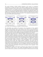
As
an example, the impact of optimizing
I,,
and
gds
simultaneously
is
shown
in
Figures
10.3
and 10.4. The ‘measured’

gds
is obtained from the
I,,
-
V,,
data by evaluating the derivative of the
I,,
-
V,,
curve at a given
V,,
using
the central difference method. The measured
Id,
-
vd,
data at
V,,
=
0
V
for a
typical 1.5 pm n-channel device (oxide thickness
=
225
A)
is
shown
as
circles

in Figure
10.3.
This data was fitted to the
SPICE
MOS
Level
3
model
[30]
by extracting the parameters using OPTIMA. In one case, only
I,,
was
optimized (conventional approach), while in the other case, both
I,,
and
g,,
were optimized simultaneously. It can be seen from Figure 10.3 that while
the current is modeled accurately through the conventional approach
(dashed lines), the slope, especially in the saturation region, does not fit
the data. This can be observed more clearly from the
gds
-
V,,
curves
(dashed lines) in Figure 10.4. On the other hand, when both
I,,
and
gds
are
optimized simultaneously, the slope is modeled more accurately (solid lines

in Figures 10.3 and 10.4).
Note that, in spite
of
optimizing the current and conductance simultaneously,
the
gd,
-
Vd,
fit (Figure 10.4) does not seem to improve significantly,
particularly near the saturation voltage
V,,,,.
This is because in the Level 3
model, the second derivative of the current
(dgd,/aV,,)
is not continuous at
520
10
Model Parameter Extraction
9.00
-
MULTIPLERE
3
0
EXPERIMEN
E
I-
Z
U
3
0

z
a
Y
m
'0
-
E
4.85
U
0
0.70
0
2.5
5
DRAIN VOLTAGE, Vd, (VOLTS)
Fig. 10.3 Comparison
of
experimental
I,,
vs.
V,,
data with the
MOS
Level
3
model
for
LDD
device with
W,/L,

=
18.75/1.5, oxide thickness
=
225
A,
V,,
=
3
V,
4V,
5
V
and
6V.
Circles
(0)
represent experimental data, dashed lines are simulated curves
from
single
response optimization and solid lines correspond to multiple response optimization
I
h
?
a
E
-
u1
D
cn
1u.u

-
1.0:
'4
,
.
.
.
,
. . .
CONVENTIONAL
MULTIPLE
RESPONSE
o
EXPERIMENTAL
0
2.5 5
DRAIN VOLTAGE, Vd,(VOLTS)
Fig.
10.4
Comparison
of
experimental
gds
vs.
V,,
curves with the MOS
Level
3
model
for

LDD
device with
W,/L,
=
18.75/1.5, oxide thickness
=
225
8,
VgE
=
4
V,
5
V
and
6
V.
Circles
(0)
represent experimental data, dashed lines are simulated curves
from
single
response
optimization and
solid
lines
correspond
to
multiple response optimization