Know and Understand Centrifugal Pumps Episode 7 docx
Bạn đang xem bản rút gọn của tài liệu. Xem và tải ngay bản đầy đủ của tài liệu tại đây (594.88 KB, 20 trang )
Know and Understand Centrifugal Pumps
Hf system piping
=
Hf suction piping+ Hf discharge piping.
=
(K
suction
x
L)
+lo0
+
(K
discharge
x
L)
+
100
=
(4.89
x
40) +lo0
+
(.637
x
140) +lo0
=
1.956
+
0.891
Hf system piping
=
2.848
feet
Now we calculate the Hf in the elbows
The formula is:
Hf elbows
=
Hf
suction elbows
+
Hf discharge elbows
=
2
x
0.280
x
0.172
+
3
x
0.310
x
0.888
=
0.096
+
0.82
Hf elbows
=
0.916
feet
Next, we calculate the Hf for the valves
There are
5
valves in all. There are
two
6
inch gate valves in the suction
pipe. There is
a
4
inch gate valve, a
4
inch globe valve, and a
4
inch
check valve in the discharge pipe. The formula is:
Hf
system valves
=
Hf suction valves
+
Hf
discharge valves
=
I(6'
gate
Hvsuction
+
I(4'
gate
HVdisch.
+
I(4'
check
HVdisch.
+
I(4'
globe
HVdisch.
=
(2
x
.09
x
0.172) +(1
x
0.16
x
0.888)
+
(1
x
2
x
0.888)
+
(1
x
6.4
x
0.888)
=
0.031
+
0.142
+
1.776
+
5.683
Hf system valves
=
7.632
feet
Next we calculate the Hf in the tramp flanges in the system
A
tramp flange is an unassociated flange or union. In the friction tables,
valves, elbows, and other fittings are categorized as
to
whether they are
flanged or screwed. This means they connect
to
the piping either by
a
bolted flange, or screwed into the pipe with male and female threading.
For example, the friction losses through a
2
inch flanged elbow, or
a
4
inch check valve, already takes into account the losses at the entrance
and exit port fittings. Then there are unassociated 'tramp' flanges and
unions. Examples would be unions between
two
lengths of pipe, or
between
a
pipe and
a
tank, or between a pipe and a pump. They must
be calculated because there is friction (and energy lost)
as
the fluid
passes through a union. In our simple system, there is a
6
inch tramp
104
The
System
Curve
flange on the suction pipe with the tank, and a
4
inch tramp with the
pump. There's
a
3
inch tramp flange
at
the pump discharge and another
4
inch tramp
at
the discharge tank. The formula is:
Hf
system tramp flanges
=
Hf
suction tramps
+
Hf
discharge
tramps
=
K5'
x
HVS"Ct.
+
I<4*
x
Hvsuct.
+
I(4"
x
HVdisch.
+
K3"
HVdisch.
=
(0)
+
(0.033
x
0.172)
+
(0.033
x
0.888)
+
(0.04
x
0.888)
=
0
+
0.005
+
0.029
+
0.035
Hf
system tramp flanges
=
0.007
feet
Admittedly, Hf of
0.007
foot is an insignificant number. Think of
it
this
way. With only one pump and
less
than
200
ft
of pipe in our simple
system, there are four tramp unions. Imagine an
oil
refinery with
20,000
pumps and thousands of miles of pipe and equipment on site.
Imagine the number of tramp flanges in the fire water system in
a
skyscraper building. In a real set of circumstances the Hf values through
tramp flnages unions could be significant, and they would have
to
be
calculated
to
specify the correct pumps.
Last, we need to calculate the
Hf
losses through other connections in
the piping
There is a sudden reduction in the suction between the tank and the
piping. There is an eccentric
6-to-4
reducer between the suction pipe
and the pump. There is
a
concentric
3-to-4
increaser from the pump
back into the piping, and a sudden enlargement going into the
discharge tank. The formula is:
Other
Hf
=
Hf
sudden
reduction
+
Hf
eccentric
reducer
+
Hf
concentric
increaser
+
Hf
sudden
enlargement
=
(0.05
x
0.172)
+
(0.28
x
0.172)
+
(0.192
x
0.888)
+
(1
x
0.888)
=
0.086
+
0.048
+
0.170
+
0.888
Other
Hf
=
1.192
feet
Now we have all the information
to
calculate the Hf in the system and
then the TDH of the system. Once again:
System
Hf
=
Hf
pipe
+
Hf
elbows
+
Hf
valves
+
Hf
flanges
+
Hf
other
=
2.848
ft
+
0.916
ft
+
7.632
ft
+
0.007
ft
+
1.192
ft
=
12.595
ft
105
1
Know and Understand Centrifugal Pumps
Consider
all
the mathematical gyrations required just
to
determine the
Hv and Hf. This is
a
lot
of math for one pump. Imagine the work
to
specify pumps for
a
paper mill or beer brewery or municipal water
system. Now you can see why governments and pharmaceutical
companies contract consulting engineering companies
to
do
this work
and specify the pumps. Finally, we can calculate the
TDH
of the
sys tem
:
TDH
=
HS
+
Hp
+
Hf
+
HV
=
80
ft
+
0
ft
+
12.595
ft
+
1.06
ft
=
93.655
ft
This system requires a pump with a best efficiency point (BEP) of
94
feet
at
300
gallons per minute. If this is a conventional industrial
centrifugal pump with a BEP of
94
feet, the shut-off head should be
approximately
110
feet. And if the motor is
a
standard NEMA four-
pole motor spinning
at
about
1800
rpm, the diameter of the impeller
should be approximately
10.5
inches. If this pump were bought off the
shelf from local distributor stock,
it
would probably be
a
3
x
4
x
12
model end-suction centrifugal back pullout pump with the impeller
machined
to
about
10.5
inches before installing the pump into the
system. And that’s the way it is done.
If the system already exists and the equipment is running, we can
recover the
Hf
and
Hv
from gauges using the Bachus
&
Custodio
Method, and forget about
all
those calculations.
See
Figure
8-8
opposite, with the corresponding elevations and placement of pressure
gauges installed into the piping numbered
1
through
5.
In this system drawing, pressure gauges
1,
2,
and
3
are in the suction
piping. Gauges
4
and
5
are in the discharge piping. With the system
and pump turned off, we would open the vent valves on both the
suction and discharge tanks, this assures that both sides of the system
are atmospheric and cancels the
Hp.
The discharge tank and all piping
should be
full
with water for the test, or if required, the pumped liquid.
Remember that gauge readings will be adjusted by the specific gravity.
Expel all air bubbles in the piping. Some pumps have a little petcock
valve
to
allow expelling any trapped air in the volute. On the pump,
conventional stuffing boxes can also trap air. This must be expelled
too.
Vertical valve stems in the piping can trap air. Loosen the packing
to
expel this trapped air. This is done
so
that there is
a
complete column of
liquid from the top
to
the bottom of the system. Air pockets and
bubbles might cause inaccurate pressure gauge readings. All valves in
the column (including the check valve) should be opened, except for
the gate valve between gauges
1
and
2.
It should be closed
to
hold the
column of liquid and prevent draining
the
line.
The
System
Curve
P
Fiaure
8-8
~
t
1
46.2'
69.3'
~
t
I
23.1'
Here's
a
quick review of the Bachus
&
Custodio Formula:
System
Wand
Hv
=
[(APDr
-
APDo)
+
(APSr
-
APSO)
x
2.311
+
sp.
gr.
Let's take our readings with water as the test liquid just to keep the
conversions simple. With the system and pump off, note that gauge
5
should be reading 20 psi. This is because it is 46.2 feet below the
surface level in the discharge tank. Confirm that gauge
4
is reading
50
psi.
It
is 115.5 feet deep into the column. The difference between
gauges
4
and
5
is
30
psi. The
APDo
=
30
psi.
In the suction
line,
note that gauge
3
is also reading
50
psi.
It
also has
11
5.5
feet
of
liquid elevation on
it.
Pressure gauge 2 should read 60 psi
because it is 138.6 feet deep into the column. This indicates that the
APSO
=
10
psi.
Gauge
1,
on the other side of the closed valve, is reading the elevation
in the suction tank. This gauge should be reading 25 psi because it is
58.6 feet deep into its column.
Now, open the gate valve between gauges
1
and
2.
Start the pump
motor, and relieve the check valve if it is being mechanically held open.
Permit the pump to run a few minutes to stabilize, relieving any
surging. We'll continue
to
note pressure gauge readings with the system
functioning.
Because all valves are now open, gauge
1
becomes our upstream gauge
on the suction line. With the pump running all activity on the suction
q
107
Know and Understand Centrifugal
Pumps
side of the pump
is
separated from the activity on the discharge side of
the pump. Gauge
1
continues
to
read 25 psi. Gauge 2 should also
record 25 psi. Gauge 3 should now be reading
15
psi, because this
gauge is 23.1 feet above gauges
1
and 2.
However, gauge 3 is recording 13 psi
(it
should be reading
15
psi) with
the system running. The APSr is 12 psi.
Gauges
1
and
2
should be reading the same pressure with the system running, as
gauge
1
was reading with the system
off.
If
you're using precision digital pressure
instrumentation gauges, gauge
2
might possibly record a fraction psi less. This is
because gauge
2
is now recording minute losses between the tank and the gauge
including losses through the opening into the pipe and the losses through the gate
valve.
If
there should be a divergence
in
the readings of the two gauges, something is out
of
control. There might be an obstruction at the tank drain line or maybe the gate valve
is not totally open. Maybe the level has dropped in the tank. Maybe the vent valve on
the tank top is not open. Maybe the gauges need calibration. Send them to a
calibration shop a couple of times per year. But, isn't
it
interesting how much more
you know about your system after learning to interpret the pressure gauges. Who is
responsible for specifying, selling, and buying pumps without adequate
instrumentation?
Now we consider the pump. We've already discussed in this book that
the pump takes the energy that the suction gives
it,
the pump adds
more energy, jacking the energy up
to
discharge pressure. In this case
the pump is designed with a
REP
of
94
feet, which also is the TDH of
the system. The
94
feet indicate that the pump can generate about
40
psi
at
300 gpm
(94
+
2.31
=
40.6
psi if the liquid
is
water). This is
confirmed with a flow meter and
a
pump curve. The suction pressure is
13
psi. The discharge pressure gauge
(4
gauge) should
be
reading 53
psi
(40
+
13).
The pump's discharge pressure is a function
of
the suction pressure. Regrettably, most
pumps in the world don't have a gauge reading suction pressure. In our example here,
if
our pump is generating less than
40
psi, the pump is operating to the right
of
its
BEP,
and is losing efficiency. Was the pump assembled correctly? Was
it
repaired
correctly, with all parts machined to their correct tolerances? Is the motor's velocity
correct?
Is
there a
flow
meter installed? The pump is always on its curve.
If
this pump
were generating more than
40
or
41
psi,
it
would be operating to the left
of
its
BEP.
Verify the other factors.
The
System
Curve
With gauge
4
on the pump discharge reading
53
psi, the
5
gauge
should be reading
30
psi less, or
23
psi. This is because the
5
gauge
is
69.3 feet above gauge
4.
However gauge
5,
by observation, is only
reading
18
psi. Therefore APDr
=
35psi
(53
-
18).
We have all the
information we need
to
insert into the Bachus
&
Custodio Formula:
Hf
&
Hv
=
(APDr
-
APDo)
+
(APSr
-
APSO)
x
2.31
i
sp.
gr.
=
(35
-
30)
+
(12
-
10)
x
2.31
i
SP.
g.
=
5
+
2
x
2.31
+
~p.gr.
=
7~ 2.31
i
1.0
Hf&Hv
=
16.17feet
The Bachus
&
Custodio Formula does
not
make mistakes.
It
is not
based on models, or experiments developed
150
years ago. It doesn’t
depend on valves being completely open.
It
doesn’t depend on the
specific instructions regarding equipment assembly. It doesn’t depend
on
new piping. It is not based on municipal water.
It
depends on the
actual piping and other system fittings, as they are now, and the next
shift, and tomorrow, and next month. If a resistance load changes, it
will be registered on the gauges. If the pipe diameter changes, it is
recorded on the gauges. If new equipment is added, it is visible on the
gauges. The pressure gauges and other instrumentation are the pump’s
control panel. You wouldn’t drive
a
car without a dashboard. Who is
responsible for spccifjring, selling and buying pumps without adequate
instrumentation? Regarding pump failure, problematic seals and
bearings that need emergency maintenance: in about
80%
of all cases,
the pump is telling the operators what the problem is, hours, days and
weeks before the failure event occurs. What’s really happening is that
no one is interpreting the information on the gauges.
Regarding the TDH, isn’t it interesting that the Hs and the Hp are
determined by simple observation? This detailed discussion on the Hf
and Hv probably has the reader ready
to
throw this book into the
garbage. With the Rachus
&
Custodio Formula, the differential
pressure gauge readings on the system with the pump turned off, will
cancel any elevation changes
(Hs)
existing in the system. Exposing both
sides
of
the system
to
atmospheric pressure cancels the pressure changes
(Hp). And then with the system operating and the pump turned on,
the further differential gauge readings will record the Hf and Hv that
are being lost in the system. Remember
too,
that the other mentioned
resistance approximations, Hazen
&
Williams, and Darcymeisbach,
are only valid in the first few hours or days of service. The system begins
to
change once the pump is turned on and production begins.
Operators open and close valves
to
meter the flow through the pipes.
Filters and strainers begin
to
clog. Inside pipe diameters form scale.
t
1109
Know and Understand Centrifugal Pumps
New
equipment
is
installed. Other changes occur with maintenance.
The equipment loses its efficiency. Install gauges on your pumps and
teach the operators and maintenance personnel to interpret the
information.
The dynamic system
Let’s continue with system curves. Up
to
this
point, all elevations,
temperatures, pressures and resistances in the drawings and graphs of
systems and tanks have been static. This is not reality. Let’s now
consider the dynamic system curve and how it coordinates with the
pump curve.
Variable elevations
In the next graph we observe
that
at
the beginning of the operation,
the lower tank is
111,
and the work of the pump is to complete the
distance between the surface level in the lower
tank
and the discharge
elevation above at the upper tank. At the end of the operation, the
lower tank is empty and the work of the pump is
to
complete the new
distance between the two elevations. Consider the next graphic (Figure
At the beginning of the operation, the work of the pump is
to
complete
elevation
Hsl.
This
elevation becomes
Hs2
at the end of the operation.
8-9).
END
BEGINNING
Figure
8-9
110
The
System
Curve
I
*
Q
GPM
0
Figure
8-11
Know and Understand Centrifugal Pumps
'A
PUMP
U
Q
BEP
Q
The System requires
X
Flow
GPM
Figure
8-12
Next, we should find a pump who's
BEP
coordinates fall right between
the
Hsl
and
Hs2
at flow
X,
as seen on the graph above (Figure 8-12).
With this
information,
the
pump curve, coordinating
with this
system's
demands according
to
the
two
tank levels, is seen
this
way (Figure 8-13).
H
BEP
1
lH
I
I
I
I
VI
0
Q
BEP
Q
t
10
GPM
Figure
8-13
The
System
Curve
The happy zone
~
Now we can
see
the importance of the concentric ellipses of efficiency
on the pump family curve.
As
much as possible we should find a pump
whose primary efficiency arc covers
the
needs of the system. Certainly
the needs of the system should fall within the second or third efficiency
arcs around the pump’s
BEP.
If the system’s needs require
the
pump
to
consistently run
too
far
to
the
left or right extremes on its curve, it may
be
best
to
consider pumps in parallel, or series, or
a
combination of the
two,
or
some other arrangement, possibly a
PD
pump. We’ll
see
this
later.
As
elevations change in the process of draining one tank and filling
another, the pump moves on its curve from
one
elevation extreme
to
the other. If we’ve selected the right pump for the system,
it
will move
from one extreme of its happy zone, through the
REP
to
the other
extreme.
This is the beginning of many problems with pumps.
A
pump is specified with the
BEP
at one set
of
system coordinates. Then the system (the TDH) goes dynamic, changing,
and the pump moves on its curve away from its
BEP
out to one or the other extreme.
It
is necessary to determine the maximum and minimum elevations in the system and
design the pump within these elevations.
If
the system continues
to
change on the
pump,
you’ll
either have to modify the system
or
modify
or
change the pump, unless
you
really like to change bearings and seals.
Dynamic pressures
Let’s consider now a system with dynamic pressures and a constant
elevation.
A
classic example of this would
be
where a pump feeds
a
sealed reactor vessel, or boiler. The fluid level in the reactor would
be
more or less static in relation
to
the pump. The resistances in the
piping, the Hf and Hv, would be mostly static although they would
go
up with flow. The Hp, pressure head would change with temperature.
Consider Figure
8-14.
The system curve, once again, is the visual graph of the four elements of
the TDH. The Hp is stacked on top of the Hs. The Hp changes with a
change in temperature in the reactor. If the reactor were cold, the Hp
would
be
minimum or zero. We’ll call this Hpl. When the tank and
fluid arc heated, the Hp rises
to
its maximum. This is represented as
Hp2 on the graph (Figure
8-15).
Know and Understand Centrifugal Pumps
H
FEET
I
0
b
Q
GPM
Let’s say that the needs of
the
system require
X
flow. Now
we
search for
a pump with a REP at
X
gpm, at a head falling right between Hpl and
Hp2 on the system curve.
See
the next graph (Figure 8-16).
The system’s AHp should fall within the pump’s primary or secondary
sweet zone. At the beginning of the operation, with the cold reactor
vessel, the pump operates
to
the right of the REP but within the sweet
zone, and as the reactor vessel is heated, the pump migrates on its curve
toward the
left,
crossing
the
BEP,
to
the other extreme of its sweet
zone. When the reaction is completed and the tank cools,
the
pump
The
System Curve
HP2
H
PI
H
FEET
I
I
I
PUMP
BEP
HERE
0
0
Q
BEP
Q
b
GPM
FLOW
X
Figure
8-16
migrates again on its curve,
this
time
toward
the
right, crossing
the
BEP
and comes
to
rest on
the
right end
of
its sweet zone.
See
the
next
graph (Figure
8-17).
HP2
Hs
Fiaure
8-1
7
HAPPY
ZONE
0
QQQ
Q
GPM
HOT BEP COLD
115
Know and Understand Centrifugal Pumps
Again, we
see
the importance of the pump family curve, with its
concentric ellipses of efficiency. It shows that in the beginning of
the operation, the pump
is
operating
to
the right of its
BEP.
As
the
pressures rise in the system, the pump moves toward the left of the
REP.
When the temperatures and pressures are reduced at the end of
the process, the pump migrates again on its curve
to
the right of the
BEP.
During the entire operation, the pump is inside its primary or
secondary sweet zone.
~
~-
-
-
Variable resistances
The Hf and
Hv
represent the resistance
losses
in the system.
Specifically, the Hf represents the energy consumed or lost due
to
friction in the system, and the Hv represents the energy consumed or
lost due
to
the velocity of the fluid moving through the system. The Hf
and the Hv are linked or connected because the Hv is used
to
calculate
the Hf. If there is no velocity in the fluid, then the fluid is not moving
through the pipes, and if the fluid is not moving through the pipes
there can be no friction between the fluid and the internal pipe walls. If
the resistance rises in
the
system, as in the case of a filter whose function
is
to
clog over time, the flow is reduced through the filter, and the
pressure or resistance rises. This means that the pump is moving toward
the left on its curve. The resistances can change in the short term, or in
the long term, with operations, with maintenance, or with
a
design
change. Let’s
see
how:
Short term resistance changes
The resistance in the pipes and system can change suddenly or in the
short term due
to
a design change, operation, or maintenance. For
example, many systems are designed incorporating variable speed
motors,
VFDs,
to
control production in
a
plant. The resistance is
multiplied
4
times simply by doubling the velocity of the fluid in
a
pipe.
Sometimes, in an existing system, the engineer orders
to
install a new
control. For example, installing a flow meter into a pipe increases the
resistance and the pump moves on its curve. In an effort
to
improve the
final product,
a
production engineer orders a change
to
the screen
meshes in the filters. This changes the Hf and the Hv in the system and
the pump migrates on its curve.
In some plants, the operators have free reins
to
govern the flow in the
pipes by opening and closing flow control valves. Strangling a valve
reduces the flow and increases the resistance and pressure in the system
The
System
Curve
in front of the valve. The pump moves away from the sweet zone of
efficiency.
In a maintenance fhction, working against
the
production clock,
someone changes a globe valve for a gate valve.
A
globe valve has
between
20
and
40
times more resistance than
a
gate valve. Someone
orders
to
exchange a bolted flanged long radius pipe elbow, with a
welded mitered
90"
elbow. This affects the resistance in the system and
the pump on its curve.
The authors recommend that all plant personnel
including the engineers, operators, and mechanics receive training to recognize these
rapid, unexpected, quick changes in a system. Some
of
these changes can be
controlled within certain limits. Others must be avoided as standard plant procedure.
Almost no one in maintenance
or
reliability relates today's failed mechanical seal
with the inoffensive change in a pipe diameter six weeks ago. Engineers should train
their personnel to understand the result of these inadvertent changes. These rapid
changes in a system are the source of pump maintenance.
~ ~~~
Long
term resistance changes
~~ ~ ~~ ~
In the long term, filters and strainers become clogged: this is their
purpose. Minerals and scale start forming on the internal pipe walls and
this reduces the interior diameters on the pipe.
A
4
inch pipe will
eventually become a
3.5
inch pipe. This moves the pump on its curve
because as the pipe diameter reduces, the velocity must increase
to
maintain flow through a smaller orifice. The Hf and Hv increase by the
square of the velocity increase.
Also
in the long term, the equipment loses its efficiency, and
replacement parts are substituted in a maintenance function.
Also,
the
plant
goes
through production expansions and contractions: new
equipment is added into
the
pipes. In short, the system and its
elevations and pressures, its resistances and velocities, are very dynamic.
The
BEP
of
the
pump is static.
What must be done is establish
the
maximum flow, and the minimum
flow, and implement controls. Regarding filters, you've got
to
establish
the flow and pressure (resistance) that corresponds
to
the new, clean
filter, and determine the flow and resistance that represents the dirty
filter and its moment for replacement. These points must be
predetermined. The visual graph of the system curve with its dynamic
resistances are seen in this example filtering and recirculating a liquid in
a tank. Consider the following graphs (Figures 8-18 and
8-19).
Know and Understand Centrifugal
Pumps
Figure
8-18
.
a
As
mentioned earlier, the system curve with the clean and dirty filters
should coincide within the sweet zone
of
the pump on
its
curve.
(Figure
8-20
and Figure
8-21).
The
System
Curve
H
FEET
CLOGGED FILTER
(Hf
+
Hv)l
NEW FILTER
Hs+Hp=O
0
0
Q
GPM
Figure
8-20
H
FEET
H
BEP
0
Fiaure
8-21
BEP GPM
The pump will run
to
the right
of
its
BEP
within its sweet zone with
the new filter, and slowly over time, move toward the left crossing the
BEP
as the filter screen clogs (Figure 8-21 and Figure 8-22).
Know and Understand Centrifugal Pumps
H
FEET
H2
H
BEP
H1
0
Fiaure
8-22
SECONDARY
PRIMARY
0
Q2
Q
Q1
Q
BEP GPM
On superimposing the curve of a single pump over this system curve,
we
see
that the system extremes are
too
wide for the pump
to
cover on
its curve (Figure
8-22).
You should install pressure sensors that transmit a message
to
shut-off
the pump, sound an alarm, or indicate
to
the operator that the moment
to
change the filter has arrived. With a new filter installed, the pump
begins operating again
to
the right of the
BEP
within the sweet zone
and slowly over time proceeds moving toward the other end of the
sweet zone.
Pumps in parallel and pumps in
series
Up
to
this point we’ve considered dynamic elements in the system with
other elements static. There are times, and systems where everything is
moving in concert together, with elevations rising and falling, variable
pressures, clogging filters, and control valves opening and closing.
When the entire system is dynamic, you’ve got
to
determine the elev-
ation extremes, the pressure extremes, and
the
resistance extremes. The
totally and completely dynamic system appears as Figure
8-23
and
Figure
8-24.
When this happens, you need
to
consider an arrangement of pumps
running in parallel, or in series, or in a combination of the
two.
Pumps
in parallel are
two
or more pumps working side by side, taking the
The
System
Curve
(Hf
+
Hv)
LOW
0
-
a
GPM
0
~~
Figure
8-23
H
FEET
Hp HIGH
Hs HIGH
i
Hp
LOW
Hs
LOW
0
Fiaure
8-24
ONE SINGLE
PUMP
CANNOT MEETTHESE
SYSTEM
NEEDS
-
a
GPM
Know and Understand Centrifugal Pumps
liquid from a common system, and discharging the liquid into the same
common system. Two pumps running in parallel offer twice the flow
at
the same head. Pumps in series are
two
or more pumps where the
discharge of one pump feeds the suction of the next pump in series.
Two pumps running in
series
offer twice the head with the same flow.
And the combination of the
two
arrangements offers up
to
multiples of
both factors. First let’s consider the arrangement of pumps in parallel.
~~
Pumps
in
parallel
The system is designed
so
that
two
equal pumps are operating together
side by side. The system can support the production of both pumps. If
the needs of production are reduced, this system can operate with only
one pump, simply by removing one pump from service (Figure
8-25).
The curves of pumps
‘A’
and
‘B’
individually, and ‘A and
B’
in parallel
are seen in Figure
8-26.
Because the system is designed for both pumps running together in
parallel, the system curve appears as shown in Figure
8-27.
Here we
see
something interesting. Because the system is designed for
both pumps running in parallel, when only one pump is operating, this
pump will run
to
the right of its
BEP.
This situation brings it’s own
peculiar set of implications, not often understood in industry.
Figure
8-25
R
122
7
The
System
Curve
PUMP CURVE
PUMPS
IN
PARALLEL PROVIDE PUMP CURVE
A
or
E
TWICETHE FLOW
A AND
B
FE&I\
‘“h
::El ~
I
oounLEs
0 0
0
GPM
-0
-
GPM
GPM
0-
H
FEET
0
-
0
Q
GPM
~ ~ ~~
Three
tips
__
-~
First,
one pump running in a parallel system tends
to
suffer from
cavitation because operation
to
the right of the
BEP
indicates that the
NPSHr of the pump rises drastically.
To
survive this condition, you
should use dual mechanical seals on these pumps. Dual
or
double
mechanical seals can withstand cavitation better than a single seal.
There is
a
discussion on this in the mechanical seal chapter of this book.
Many engineers perceive that parallel pumps are problematic because
they appear
to
suffer a
lot
of premature seal failure. Parallel pumps
deserve double seals even if it’s only
a
cold water system.
The
solution
is:
Parallel pumps should have dual or double seals
installed
to
withstand cavitation when one pump is running solo.