Advanced Methods and Tools for ECG Data Analysis - Part 5 pdf

P1: Shashi
August 30, 2006 11:5 Chan-Horizon Azuaje˙Book
5.3 Wavelet Filtering 145
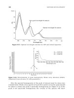
Figure 5.5 The effect of a selection of different wavelets for filtering a section of ECG (using the
first approximation only) contaminated by Gaussian pink noise (SNR = 20 dB). From top to bottom;
original (clean) ECG, noisy ECG, biorthogonal (8,4) filtered, discrete Meyer filtered, Coiflet filtered,
symlet (6,6) filtered, symlet filtered (4,4), Daubechies (4,4) filtered, reverse biorthogonal (3,5), re-
verse biorthogonal (4,8), Haar filtered, and biorthogonal (6,2) filtered. The zero-noise clean ECG is
created by averaging 1,228 R-peak aligned, 1-second-long segments of the author’sECG. RMS error
performance of each filter is listed in Table 5.1.
to the length of the highpass filter. Therefore Matlab’s bior4.4 has four vanishing
moments
3
with 9 LP and 7 HP coefficients (or taps) in each of the filters.
Figure 5.5 illustrates the effect of using different mother wavelets to filter
a section of clean (zero-noise) ECG, using only the first approximation of each
wavelet decomposition. The clean (upper) ECG is created by averaging 1,228
R-peak aligned, 1-second-long segments of the author’s ECG. Gaussian pink noise
is then added with a signal-to-noise ratio (SNR) of 20 dB. The root mean square
(RMS) error between the filtered waveform and the original clean ECG for each
wavelet is given in Table 5.1. Note that the biorthogonal wavelets with J ,K ≥ 8, 4,
3.
If the Fourier transform of the wavelet is J continuously differentiable, then the wavelet has J vanishing
moments. Type wavei n f o(

bi or

) at the Matlab prompt for more information. Viewing the filters using
[lp
decon
, hp

decon
, lp
recon
, hp
recon
] = wfilters(

bi or 4.4

) in Matlab reveals one zero coefficient in each of
the LP decomposition and HP reconstruction filters, and three zeros in the LP reconstruction and HP
decomposition filters. Note that these zeros are simply padded and do not count when calculating the filter
size.
P1: Shashi
August 30, 2006 11:5 Chan-Horizon Azuaje˙Book
146 Linear Filtering Methods
Table 5.1 Signals Displayed in Figure 5.5 (from Top to Bottom)
with RMS Error Between Clean and Wavelet Filtered ECG with 20-dB
Additive Gaussian Pink Noise
Wavelet Family Family Member RMS Error
Original ECG N/A 0
ECG with pink noise N/A 0.3190
Biorthogonal ‘bior’ bior3.3 0.0296
Discrete Meyer ‘dmey’ dmey 0.0296
Coiflets ‘coif’ coif2 0.0297
Symlets ‘sym’ sym3 0.0312
Symlets ‘sym’ sym2 0.0312
Daubechies ‘db’ db2 0.0312
Reverse biorthogonal ‘rbio’ rbio3.3 0.0322
Reverse biorthogonal ‘rbio’ rbio2.2 0.0356

Haar ‘haar’ haar 0.0462
Biorthogonal ‘bior’ bior1.3 0.0472
N/A indicates not applicable.
the discrete Meyer wavelet and the Coiflets appear to produce the best filtering
performance in this circumstance. The RMS results agree with visual inspection,
where significant morphological distortions can be seen for the other filtered sig-
nals. In general, increasing the number of taps in the filter produces a lower error
filter.
The wavelet transform can be considered either as a spectral filter applied over
many time scales, or viewed as a linear time filter [(t −τ)/a] centered at a time τ
with scale a that is convolved with the time series x(t). Therefore, convolving the
filters with a shape more commensurate with that of the ECG produces a better
filter. Figure 5.4 illustrates this point. Note that as we increase the number of taps
in the filter, the mother wavelet begins to resemble the ECG’s P-QRS-T morphol-
ogy more closely. The biorthogonal wavelet family members are FIR filters and,
therefore, possess a linear phase response, which is an important characteristic for
signal and image reconstruction. In general, biorthogonal spline wavelets allow ex-
act reconstruction of the decomposed signal. This is not possible using orthogonal
wavelets (except for the Haar wavelet). Therefore, bi or 3.3 is a good choice for a
general ECG filter. It should be noted that the filtering performance of each wavelet
will be different for different types of noise, and an adaptive wavelet-switching pro-
cedure may be appropriate. As with all filters, the wavelet performance may also
be application-specific, and a sensitivity analysis on the ECG feature of interest is
appropriate (e.g., QT interval or ST level) before selecting a particular wavelet.
As a practical example of comparing different common filtering types to the
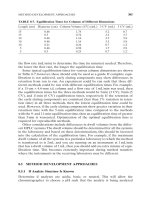
ECG, observe Figure 5.6. The upper trace illustrates an unfiltered recording of a
V5 ECG lead from a 30-year-old healthy adult male undergoing an exercise test.
Note the presence of high amplitude 50-Hz (mains) noise. The second subplot
illustrates the action of applying a 3-tap IIR notch-filter centered on 50 Hz, to
reveal the underlying ECG. Note the presence of baseline wander disturbance from

electrode motion around t = 467 seconds, and the difficulty in discerning the P wave
(indicated by a large arrow at the far left). The third trace is a band-pass (0.1 to
45 Hz) FIR filtered version of the upper trace. Note the baseline wander is reduced
P1: Shashi
August 30, 2006 11:5 Chan-Horizon Azuaje˙Book
5.3 Wavelet Filtering 147
Figure 5.6 Raw ECG with 50 Hz mains noise, IIR 50-Hz notch filtered ECG, 0.1- to 45-Hz band-
pass filtered ECG and bior3.3 wavelet filtered ECG. The left-most arrow indicates the low amplitude
P wave. Central arrows indicate Gibbs oscillations in the FIR filter causing a distortion larger than the
P wave.
significantly, but a Gibbs
4
ringing phenomena is introduced into the Q and S waves
(illustrated by the small arrows), which manifests as distortions with an amplitude
larger than the P wave itself. A good demonstration of the Gibbs phenomenon
can be found in [9, 10]. This ringing can lead to significant problems for a QRS
detector (looking for Q wave onset) or any technique for analyzing at QT intervals
or ST changes. The lower trace is the first approximation of a biorthogonal wavelet
decomposition (bior3.3) of the notch-filtered ECG. Note that the P wave is now
discernible from the background noise and the Gibbs oscillations are not present.
As mentioned at the start of this section, the number of articles on ECG analysis
that employ wavelets is enormous and an excellent overview of many of the key
publications in this arena can be found in Addison [5]. Wavelet filtering is a lossless
supervised filtering method where the basis functions are chosen a priori, much
like the case of a Fourier-based filter (although some of the wavelets do not have
orthogonal basis functions). Unfortunately, it is difficult to remove in-band noise
because the CWT and DWT are signal separation methods that effectively occur in
4.
The existence of the ripples with amplitudes independent of the filter length. Increasing the filter length
narrows the transition width but does not affect the ripple. One technique to reduce the ripples is to multiply

the impulse response of an ideal filter by a tapered window.
P1: Shashi
August 30, 2006 11:5 Chan-Horizon Azuaje˙Book
148 Linear Filtering Methods
the frequency domain
5
(ECG signal and noises often have a significant overlap in the
frequency domain). In the next section we will look at techniques that discover the
basis functions within data, based either on the statistics of the signal’s distributions
or with reference to a known signal model. The basis functions may overlap in the
frequency domain, and therefore, we may separate out in-band noise.
As a postscript to this section, it should be noted that there has been much
discussion of the use of wavelets in HRV analysis (see Chapter 3) since long-range
beat-to-beat fluctuations are obviously nonstationary. Unfortunately, very little at-
tention has been paid to the unevenly sampled nature of the RR interval time series
and this can lead to serious errors (see Chapter 3). Techniques for wavelet analy-
sis of unevenly sampled data do exist [11, 12], but it is not clear how a discrete
filter bank formulation with up-down sampling could avoid the inherent problems
of resampling an unevenly sampled signal. A recently proposed alternative JTFA
technique known as the Hilbert-Huang transform (HHT) [13, 14], which is based
upon empirical mode decomposition (EMD), has shown promise in the area of non-
stationary and nonlinear JFTA (since both the amplitude and frequency terms are
a function of time
6
). Furthermore, there is striking similarity between EMD and
the least-squares estimation technique used in calculating the Lomb-Scargle Peri-
odogram (LSP) for power spectral density estimation of unevenly sampled signals
(see Chapter 3). EMD attempts to find basis functions (such as the sines and cosines
in the LSP) by fitting them to the signal and then subtracting them, in much the
same manner as in the calculation of the LSP (with the difference being that EMD

analyzes the envelope of the signal and does not restrict the basis functions to be-
ing sinusoidal). It is therefore logical to extend the HHT technique to fit empirical
modes to an unevenly sampled times series such as the RR tachogram. If the fit is
optimal in a least-squares sense, then the basis functions will remain orthogonal (as
we shall discover in the next section). Of course, the basis functions may not be
orthogonal, and other measures for optimal fits may be employed. This concept is
explored further in Section 5.4.3.2.
5.4 Data-Determined Basis Functions
Sections 5.4.1 to 5.4.3 present a set of transformation techniques for filtering or
separating signals without using any prior knowledge of the spectral components
of the signals and are based upon a statistical analysis to discover the underlying
basis functions of a set of signals.
These transformation techniques are principal component analysis
7
(PCA),
artificial neural networks (ANNs), and independent component analysis (ICA).
5.
The wavelet is convolved with the signal.
6.
Interestingly, the empirical modes of the HHT are also determined by the data and are therefore a special
case where a JTFA technique (the Hilbert transform) is combined with a data-determined empirical mode
decomposition to derive orthogonal basis functions that may overlap in the frequency domain in a nonlinear
manner.
7.
This is also known as singular value decomposition (SVD), the Hotelling transform or the Karhunen-Lo
`
eve
transform (KLT).
P1: Shashi
September 4, 2006 10:25 Chan-Horizon Azuaje˙Book

5.4 Data-Determined Basis Functions 149
Both PCA and ICA attempt to find an independent set of vectors onto which we
can transform data. Those data that are projected (or mapped) onto each vector
are the independent sources. The basic goal in PCA is to decorrelate the signal by
projecting data onto orthogonal axes. However, ICA results in a transformation of
data onto a set of axes which are not necessarily orthogonal. Both PCA and ICA can
be used to perform lossy or lossless transformations by multiplying the recorded
(observation) data by a separation or demixing matrix. Lossless PCA and ICA
both involve projecting data onto a set of axes which are determined by the nature
of those data, and are therefore methods of blind source separation (BSS). (Blind
because the axes of projection and therefore the sources are determined through the
application of an internal measure and without the use of any prior knowledge of
a signal’s structure.)
Once we have discovered the axes of the independent components in a data set
and have separated them out by projecting the data set onto these axes, we can then
use these techniques to filter the data set.
5.4.1 Principal Component Analysis
To determine the principal components (PCs) of a multidimensional signal, we can
use the method of singular value decomposition. Consider a real N × M matrix X
of observations which may be decomposed as follows:
X = USV
T
(5.8)
where S is an N × M nonsquare matrix with zero entries everywhere, except on the
leading diagonal with elements s
i
(= S
nm
, n = m) arranged in descending order of
magnitude. Each s

i
is equal to
√
λ
i
, the square root of the eigenvalues of C = X
T
X.
A stem-plot of these values against their index i is known as the singular spectrum.
The smaller the eigenvalues are, the less energy along the corresponding eigenvector
there is. Therefore, the smallest eigenvalues are often considered to be associated
with the noise in the signal. V is an M × M matrix of column vectors which are the
eigenvectors of C. U is an N×N matrix of projections of X onto the eigenvectors of
C [15]. If a truncated SVD of X is performed (i.e. we just retain the most significant
p eigenvectors),
8
then the truncated SVD is given by Y = US
p
V
T
, and the columns
of the N × M matrix Y are the noise-reduced signal (see Figure 5.7).
SVD is a commonly employed technique to compress and/or filter the ECG.
In particular, if we align M heartbeats, each N samples long, in a matrix (of size
N × M), we can compress it down (into an N × p) matrix, using only the first
p << M PCs. If we then reconstruct the set of heartbeats by inverting the reduced
rank matrix, we effectively filter the original ECG.
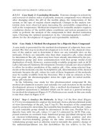
Figure 5.7(a) illustrates a set of 20 heartbeat waveforms which have been cut
into 1-second segments (with a sampling frequency F
s

= 256 Hz), aligned by their
R peaks and placed side by side to form a 256 × 20 matrix. Therefore, the data
set is 20-dimensional, and an SVD will lead to 20 eigenvectors. Figure 5.7(b) is
8.
In practice choosing the value of p depends on the nature of the data set, but is often taken to be the knee
in the eigenspectrum or as the value where

p
i=1
s
i
>α

M
i=1
s
i
and α is some fraction ≈ 0.95.
P1: Shashi
August 30, 2006 11:5 Chan-Horizon Azuaje˙Book
150 Linear Filtering Methods
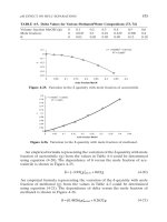
Figure 5.7 SVD of 20 R-peak-aligned P-QRS-T complexes: (a) in the original form with in-band
Gaussian pink noise noise (SNR = 14 dB), (b) eigenspectrum of decomposition (with the knee
indicated by an arrow), (c) reconstruction using only the first principal component, and (d) recon-
struction using only the first two principal components.
the eigenspectrum obtained from SVD.
9
Note that the signal/noise boundary is
generally taken to be the knee of the eigenspectrum, which is indicated by an ar-
row in Figure 5.7(b). Since the eigenvalues are related to the power, most of the

power is contained in the first five eigenvectors (in this example). Figure 5.7(c) is a
plot of the reconstruction (filtering) of the data set using just the first eigenvector.
Figure 5.7(d) is the same as Figure 5.7(c), but the first five eigenvectors have been
used to reconstruct the data set.
10
The data set in Figure 5.7(d) is therefore noisier
than that in Figure 5.7(c), but cleaner than that in Figure 5.7(a). Note that although
Figure 5.7(c) appears to be extremely clean, this is at the cost of removing some
beat-to-beat morphological changes, since only one PC was used.
Note that S derived from a full SVD is an invertible matrix, and no information
is lost if we retain all the PCs. In other words, we recover the original data by
performing the multiplication USV
T
. However, if we perform a truncated SVD,
then the inverse of S does not exist. The transformation that performs the filtering
is noninvertible, and information is lost because S is singular.
From a data compression point of view, SVD is an excellent tool. If the eigenspace
is known (or previously determined from experiments), then the M-dimensions of
9.
In Matlab: [USV] = svd(data); stem(diag(S)
2
).
10.
In Matlab: [USV] = svds(data,5);water f all(U ∗ S ∗ V

).
P1: Shashi
August 30, 2006 11:5 Chan-Horizon Azuaje˙Book
5.4 Data-Determined Basis Functions 151
data can in general be encoded in only p-dimensions of data. So for N sample points

in each signal, an N×M matrix is reduced to an N×p matrix. In the above example,
retaining only the first principal component, we achieve a compression ration of
20:1. Note that the data set is encoded in the U matrix, so we are only interested
in the first p columns. The eigenvalues and eigenvectors are encoded in S and V
matrices, and thus an additional p scalar values are required to encode the relative
energies in each column (or signal source) in U. Furthermore, if we wish to encode
the eigenspace onto which the data set in U is projected, we require an additional
p
2
scalar values (the elements of V). Therefore, SVD compression only becomes
of significant value when a large number of beats are analyzed. It should be noted
that the eigenvectors will change over time since they are based upon the morphol-
ogy of the beats. Morphology changes both subtly with heart rate–related cardiac
conduction velocity changes, and with conduction path abnormalities that produce
abnormal beats. Furthermore, the basis functions are lead dependent, unless a mul-
tidimensional basis function set is derived and the leads are mapped onto this set. In
order to find the global eigenspace for all beats, we need to take a large, representa-
tive set of heartbeats
11
and perform SVD upon this training set [16, 17]. Projecting
each new beat onto these globally derived basis vectors leads to a filtering of the
signal that is essentially equivalent to passing the P-QRS-T complex through a set
of trained weights of a multilayer perceptron (MLP) neural network (see [18] and
the following section). Abnormal beats or artifacts erroneously detected as normal
beats will have abnormal eigenvalues (or a highly irregular structure when recon-
structed by the MLP). In this way, beat classification can be performed. However, in
order to retain all the subtleties of the QRS complex, at least p = 5 eigenvalues and
eigenvectors are required (and another five for the rest of the beat). At a sampling
frequency of F
s

Hz and an average beat-to-beat interval of RR
av
(or heart rate of
60/RR
av
), the compression ratio is F
s
· RR
av
· (
N−p
p
) : 1, where N is the number
of samples in each segmented heartbeat. Other studies have used between 10 [19]
and 16 [18] free parameters (neurons) to encode (or model) each beat, but these
methods necessarily model some noise also.
In Chapter 9 we will see how we can derive a global set of principal eigenvectors
V (or KL basis functions) onto which we can project each beat. The strength of the
projection along each eigenvector
12
allows us to classify the beat type. In the next
section, we will look at an online adaptive implementation of this technique for
patient-specific learning, using the framework of artificial neural networks.
5.4.2 Neural Network Filtering
PCA can be reformulated as a neural network problem, and, in fact, a MLP with
linear activation functions can be shown to perform singular valued decomposition
[18, 20]. Consider an auto-associative multilayered perceptron (AAMLP) neural
network, which has as many output nodes as input nodes, illustrated in Figure 5.8.
The AAMLP can be trained using an objective cost function measured between the
11.

That is, N >> 20.
12.
Derived from a database of test signals.
P1: Shashi
August 30, 2006 11:5 Chan-Horizon Azuaje˙Book
152 Linear Filtering Methods
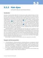
Figure 5.8 Layout of a D-p-D auto-associative neural network.
inputs and outputs; the target data vector is simply the input data vector. There-
fore, no labeling of training data is required. An auto-associative neural network
performs dimensionality reduction from D to p dimensions (D > p) and then
projects back up to D dimensions. (See Figure 5.8.) PCA, a standard linear dimen-
sionality reduction procedure is also a form of unsupervised learning [20]. In fact,
the number of hidden-layer nodes ( dim(y
j
) ) is usually chosen to be the same as
the number of PCs, p, in the data set (see Section 5.4.1), since (as we shall see later)
the first layer of weights performs PCA if trained with a linear activation function.
The full derivation of PCA shows that PCA is based on minimizing a sum-of-squares
error cost function, as is the case for the AAMLP [20].
The input data used to train the network is now defined as y
i
for consistency of
notation. The y
i
are fed into the network and propagated through to give an output
y
k
given by
y
k

= f
a



j
w
jk
f
a
(

i
w
ij
y
i
)


(5.9)
where f
a
is the activation function,
13
a
j
=

i=N

i=0
w
ij
y
i
, and D = N is the number
of input nodes. Note that the x’s from the previous section are now the y
i
, our
sources are the y
j
, and our filtered data (after training) are the y
k
. During training,
the target data vector or desired output, t
k
, which is associated with the training
data vector, is compared to the actual output y
k
. The weights, w
jk
and w
ij
, are then
adjusted in order to minimize the difference between the propagated output and the
target value. This error is defined over all training patterns, M, in the training set as
ξ =
1
2
M


n=1

k


f
a
(

j
w
jk
f
a
(

i
w
ij
y
p
i
)) − t
p
k


2
(5.10)

where j = p is the number of hidden units and ξ is the error to be backpropagated
at each learning cycle. Note that the y
j
are the values of the data set after projection
13.
Often taken to be a sigmoid ( f
a
(a) =
1
1+e
−a
), a tanh,orasoftmax function).
P1: Shashi
August 30, 2006 11:5 Chan-Horizon Azuaje˙Book
5.4 Data-Determined Basis Functions 153
onto the p-dimensional (p < N, D) hidden layer (the PCs). This is the point at
which the dimensionality reduction (and hence filtering) really occurs, since the
input dimensionality equals the output dimensionality (N = D).
The squared error, ξ , can be minimized using the method of gradient descent
[20]. This requires the gradient to be calculated with respect to each weight, w
ij
and w
jk
. The weight update equations for the hidden and output layers are given
as follows:
w
(τ+1)
jk
= w
(τ)

jk
− η
∂ξ
∂w
jk
(5.11)
w
(τ+1)
ij
= w
(τ)
ij
− η
∂ξ
∂w
ij
(5.12)
where τ represents the iteration step and η is a small (<< 1) learning term. In
general, the weights are updated until ξ reaches some minimum. Training is an
iterative process [repeated application of (5.11) and (5.12)], but, if continued for
too long,
14
the network starts to fit the noise in the training set and that will
have a negative effect on the performance of the trained network on test data.
The decision on when to stop training is of vital importance but is often defined
when the error function (or its gradient) drops below some predefined level. The
use of an independent validation set is often the best way to decide on when to
terminate training (see Bishop [20, p. 262] for more details). However, in the case
of an auto-associative network, no validation set is required, and the training can
be terminated when the ratio of the variance of the input and output data reaches

a plateau. (See [21, 22].)
If f
a
is set to be linear y
k
= a
k
,
∂y
k
∂a
k
= 1, then the expression for δ
k
reduces to
δ
k
=
∂ξ
∂a
k
=
∂ξ
∂y
k
·
∂y
k
∂a
k

= (y
k
− t
k
) (5.13)
If the hidden layer also contains linear units, further changes must be made to the
weight update equations:
δ
j
=
∂ξ
∂a
j
=
∂ξ
∂a
k
·
∂a
k
∂y
j
·
∂y
j
∂a
j
=

k

δ
k
w
jk
(5.14)
If f
a
is linearized (set to unity)—this expression is differentiated with respect to
w
ij
and the derivative is set to zero, the usual equations for least-squares optimiza-
tion can be given in the form
M

M

D

i

=0
y
m
i
w
i

j
− t
m

j

y
m
i
= 0 (5.15)
14.
Note that a momentum term can be inserted into (5.11) and (5.12) to premultiply the weights and increase
the speed of convergence of the network.
P1: Shashi
September 4, 2006 10:29 Chan-Horizon Azuaje˙Book
154 Linear Filtering Methods
which is written in matrix notation as
(Y
T
Y)W
T
= Y
T
T (5.16)
Y has dimensions M × D with elements y
m
i
where M is the number of training
patterns and D the number of input nodes to the network (the length of each ECG
complex in our examples). W has dimension p × D and elements w
ij
and T has
dimensions M × p and elements t
m

j
. The matrix (Y
T
Y) is a square p × p matrix
which may be inverted to obtain the solution
W
T
= Y
†
T (5.17)
where Y
†
is the (p × M) pseudo-inverse of Y and is given by
Y
†
= (Y
T
Y)
−1
Y
T
(5.18)
Note that in practice (Y
T
Y) usually turns out to be near-singular and SVD is used
to avoid problems caused by the accumulation of numerical roundoff errors.
Consider M training patterns, each i = N samples long presented to the auto-
associative MLP with i input and k output nodes (i = k) and j ≤ i hidden nodes.
For the mth (m = 1 M) input vector x
i

of the i × M (M ≥ i) real input matrix,
X, formed by the M (i-dimensional) training vectors, the hidden unit output values
are
h
j
= f
a
(W
1
x
i
+ w
1b
) (5.19)
where W
1
is the input-to-hidden layer i × j weight matrix, w
1b
is a rank- j vector
of biases, and f
a
is an activation function. The output of the auto-associative MLP
can then be written as
y
k
= W
2
h
j
+ w

2b
(5.20)
where W
2
is the hidden-to-output layer j × k weight matrix and w
2b
is a rank-k
vector of biases. Now consider the singular value decomposition of X, such that
X
i
= U
i
S
i
V
T
i
, where U is an i ×i column-orthogonal matrix, S is an i ×N diagonal
matrix with positive or zero elements (the singular values) and V
T
is the transpose
of an N×N orthogonal matrix [15]. The best rank- j approximation of X is W
2
h
j
=
U
j
S
j

V
T
j
[23], where
h
j
= FS
j
V
T
j
(5.21)
W
2
= U
j
F
−1
(5.22)
with F being an arbitrary nonsingular j × j scaling matrix. U
j
has i × j elements,
S
j
has j × j elements, and V
T
has j × M elements. It can be shown that [24]
W
1
= a

−1
1
FU
T
j
(5.23)
P1: Shashi
August 30, 2006 11:5 Chan-Horizon Azuaje˙Book
5.4 Data-Determined Basis Functions 155
where W
1
are the input-to-hidden layer weights and a is derived from a power
series expansion of the activation function, f
a
(x) ≈ a
0
+ a
1
x for small x. For a
linear activation function, as in this application, a
0
= 0, a
1
= 1. The bias weights
given in [24] reduce to
w
1b
=−a
−1
1

FU
T
j
µ
X
=−U
T
j
µ
X
w
2b
= µ
X
− a
0
U
j
F
−1
= µ
X
(5.24)
where µ
X
=
1
M

M

x
i
, the average of the training (input) vectors and F is here set
to be the ( j × j) identity matrix since the output is unaffected by the scaling. Using
(5.19) to (5.24),
y
k
= W
2
h
j
+ w
2b
= U
j
F
−1
h
j
+ w
2b
(5.25)
= U
j
F
−1
(W
1
x
i

+ w
1b
) + w
2b
= U
j
F
−1
1
FU
T
j
x
i
− U
j
F
−1
U
T
j
µ
X
+ µ
X
giving the output of the auto-associative MLP as
y
k
= U
j

U
T
j
(X − µ
X
) + µ
X
(5.26)
Equations (5.22), (5.23), and (5.24) represent an analytical solution to deter-
mine the weights of the auto-associative MLP “in one pass” over the input (train-
ing) data with as few as Mi
3
+6Mi
2
+O(Mi ) multiplications [25]. We can see that
W
1
= W
ij
is the matrix that rotates each of the data vectors x
m
i
= y
m
i
in X into
the hidden data y
p
i
, which are our p underlying sources. W

2
= W
jk
is the matrix
that transforms our sources back into the observation data; the target data vectors

N
t
m
i
= T.If p < N, we have discarded some of the possible information sources
and effected a filtering process. In terms of PCA, W
1
= SV
T
= UU
T
.
5.4.2.1 Determining the Network Architecture for Filtering
It is now simple to see how we can derive an heuristic for determining the MLP’s
architecture: the number of input, hidden, and output units, the activation function,
and the cost function. A general method is as follows [26]:
1. Choose the number of input units based upon the type of signal requiring
analysis, and reduce the number of them as far as possible. (Downsample
the signal as far as possible without removing significant information.)
2. Choose the number of output units based upon how many classes that are
to be distinguished. (In the application in this chapter the filtering preserves
the sampling frequency of the original signal, so the number of output units
must equal the number of input units and hence the input is reconstructed
in a filtered form at the output.)

3. Choose the number of hidden units based upon how amenable the data
set is to compression. If the activation function is linear, then the choice is
obvious; we use the knee of the SVD eigenspectrum (see Figure 5.7).
P1: Shashi
August 30, 2006 11:5 Chan-Horizon Azuaje˙Book
156 Linear Filtering Methods
5.4.2.2 ECG Filtering
To reconstruct the ECG (minus the noise component), we set the number of hidden
nodes to be the same as the number of PCs required to encode the information
in the ECG (p = 5 or 6); see Chapter 9 and Moody et al. [16, 17]. Setting the
number of output nodes to equal the number of input nodes (i.e., the number of
samples in the segmented P-QRS-T wave) results in an auto-associative MLP which
reconstructs the ECG with p PCs. That is, the trained neural network filters the
ECG. To train the weights of the system we can present a series of patterns to the
MLP and back propagate the error between the pattern and the output of the MLP,
which should be the same, until the variance of the input over the variance of the
output approaches unity. We can also use (5.22), (5.23), (5.24), and SVD to set the
values of the weights.
Once an MLP is trained to filter the ECG in this way, we may update the
weights periodically with new patterns
15
and continually track the morphology to
produce a more generalized filter, as long as we take care to exclude artifacts.
16
It
has been suggested [24] that sequential SVD methods [25] can be used to update
U. However, at least 12i
2
+O
(i) multiplications are required for each new training

vector, and therefore, it is only a preferable update scheme when there is a large
difference between the new patterns and the old training set (M or i are then large).
For normal ECG morphologies, even in extreme circumstances such as increasing
ST elevation, this is not the case.
Another approach is to determine a global set of PCs (or KL basis functions)
over a range of patients and attempt to classify each beat sequentially by clustering
the eigenvalues (KL coefficients) in the KL space. See [16, 17] and Chapter 9 for a
more in-depth analysis of this.
Of course, so far there is no advantage to formulating the PCA filtering as a
neural network problem (unless the activation function is made nonlinear). The
key point we are illustrating by reformulating the PCA approach in terms of the
ANN learning paradigm is that PCA and ICA are intimately connected. By using a
linear activation function, we are assuming that the latent variables that generate
our underlying sources are Gaussian. Furthermore, the mean square error–based
function leads to orthogonal axes. The reason for starting with PCA is that it offers
the simplest computational route, and a direct interpretation of the basis func-
tions; they are the axes of maximal variance in the covariance matrix. As soon
as we introduce a nonlinear activation function, we lose an exact interpretation
of the axes. However, if the activation function is chosen to be nonlinear, then
we are implicitly assuming non-Gaussian sources. Choosing a tanh-like function
implies heavy-tailed sources, which is probably the case for the cardiac source
itself, and therefore is perhaps a better choice for deriving representative basis
functions.
Moreover, by replacing the cost function with entropy-based function, we can
remove the constraint of second-order (variance-based) independence, and hence
15.
With just a few (∼ 10) iterations through the backpropagation algorithm.
16.
Note also that a separate network is required for each beat type on each lead, and therefore a beat classifi-
cation system is required.

P1: Shashi
August 30, 2006 11:5 Chan-Horizon Azuaje˙Book
5.4 Data-Determined Basis Functions 157
orthogonality between the basis functions. In this way, a more effective filter may
be formulated. As we shall see in the next section, it can be shown [27] that if
this cost function is changed to become some mutual information-based criterion,
then the basis function independence becomes fourth order (in a statistical sense)
and the basis-function orthogonality is lost. We are no longer performing PCA, but
rather ICA.
5.4.3 Independent Component Analysis for Source Separation
and Filtering
Using PCA (or its AAMLP correlate) we have seen how we can separate a signal
into a subspace that is signal and a subspace that is essentially noise. This is done
by assuming that only the eigenvectors associated with the p largest eigenvalues
represent the signal, and the remaining (M − p) eigenvalues are associated with
the noise subspace. We try to maximize the independence between the eigenvectors
that span these subspaces by requiring them to be orthogonal. However, orthogonal
subspaces may not be the best way to differentiate between the constituent sources
(signal and noise) in a set of observations.
In this section, we will examine how choosing a measure of independence other
than variance can lead to a more effective method for separating signals. The method
will be presented in a gradient-descent formulation in order to illustrate the connec-
tions with AANN’s and PCA. A detailed description of how ICA can be implemented
using gradient descent, which follows closely the work of MacKay [27], is given in
the material on the accompanying URLs [28, 29]. Rather than provide this detailed
description here, an intuitive description of how ICA separates sources is presented,
together with a practical application to noise reduction.
A particularly intuitive illustration of the problem of blind
17
source separation

through discovering independent sources is known as the Cocktail Party
Problem.
5.4.3.1 Blind Source Separation: The Cocktail Party Problem
The Cocktail Party Problem refers to the separation of a set of observations (the
mixture of conversations one hears in each ear) into the constituent underlying
(statistically independent) source signals. If each of the J speakers (sources) that
are talking in a room at a party is recorded by M microphones,
18
the recordings
can be considered to be a matrix composed of a set of M vectors,
19
each of which
is a (weighted) linear superposition of the J voices. For a discrete set of N samples,
we can denote the sources by a J × N matrix, Z, and the M recordings by an
M × N matrix X. Z is therefore transformed into the observables X (through the
propagation of sound waves through the room) by multiplying it by an M × J
mixing matrix A, such that X
T
= AZ
T
. [Recall (5.2).]
17.
Since we discover, rather than define, the subspace onto which we project the data set, this process is known
as blind source separation (BSS). Therefore, PCA can also be thought of as a BSS technique.
18.
In the case of a human, the ears are the M = 2 microphones.
19.
M is usually required to be greater than or equal to J .
P1: Shashi
September 4, 2006 10:39 Chan-Horizon Azuaje˙Book

158 Linear Filtering Methods
In order for us to pick out a voice from an ensemble of voices in a crowded
room, we must perform some type of BSS to recover the original sources from the
observed mixture. Mathematically, we want to find a demixing matrix W, which
when multiplied by the recordings X, produces an estimate Y of the sources Z.
Therefore, W is a set of weights (approximately equal
20
)toA
−1
. One of the key
BSS methods is ICA, where we take advantage of (an assumed) linear independence
between the sources. In the case of ECG analysis, the independent sources are
assumed to be the electrocardiac signal and exogenous noises (such as muscular
activity or electrode movement).
5.4.3.2 Higher-Order Independence: ICA
ICA is a general name for a variety of techniques that seek to uncover the (statis-
tically) independent source signals from a set of observations that are composed of
underlying components that are usually assumed to be mixed in a linear and station-
ary manner. Consider X
jn
to be a matrix of J observed random vectors: A,anN× J
mixing matrix, and Z, the J (assumed) source vectors, which are mixed such that
X
T
= AZ
T
(5.27)
Note that here we have chosen to use the transposes of X and Z to retain dimen-
sional consistency with the PCA formulation in Section 5.4.1, (5.8). ICA algorithms
attempt to find a separating or demixing matrix W such that

Y
T
= WX
T
(5.28)
where W =
ˆ
A
−1
, an approximation of the inverse of the original mixing matrix,
and Y
T
=
ˆ
Z
T
,anM × J matrix, is an approximation of the underlying sources.
These sources are assumed to be statistically independent (generated by unrelated
processes) and therefore the joint probability density function (PDF) is the product
of the densities for all sources:
P(Z) =

p(z
i
) (5.29)
where p(z
i
) is the PDF of the ith source and P(Z) is the joint density function.
The basic idea of ICA is to apply operations to the observed data X
T

, or the
demixing matrix W, and measure the independence between the output signal chan-
nels (the columns of Y
T
) to derive estimates of the sources (the columns of Z
T
). In
practice, iterative methods are used to maximize or minimize a given cost func-
tion such as mutual information, entropy, or the fourth-order moment, kurtosis,a
measure of non-Gaussianity (see Section 5.4.3.3). It can be shown [27] that entropy-
based cost functions are related to kurtosis, and therefore, all of the cost functions
used in ICA are a measure of non-Gaussianity to some extent.
21
20.
Depending on the performance details of the algorithm used to calculate W.
21.
The reason for choosing between different entropy-based cost functions is not always made clear, but com-
putational efficiency and sensitivity to outliers are among the concerns. See material on the accompanying
URLs [28, 29] for more information.
P1: Shashi
August 30, 2006 11:5 Chan-Horizon Azuaje˙Book
5.4 Data-Determined Basis Functions 159
From the Central Limit Theorem [30], we know that the distribution of a sum
of independent random variables tends toward a Gaussian distribution. That is, a
sum of two independent random variables usually has a distribution that is closer to
a Gaussian than the two original random variables. In other words, independence
is non-Gaussianity. For ICA, if we wish to find independent sources, we must find a
demixing matrix W, that maximizes the non-Gaussianity of each source. It should
also be noted at this point that, for the sake of simplicity, this chapter uses the con-
vention J ≡ M, so that the number of sources equals the dimensionality of the signal

(the number of independent observations). If J < M, it is important to attempt to
determine the exact number of sources in a signal matrix. For more information on
this topic see the articles on relevancy determination [31, 32]. Furthermore, with
conventional ICA, we can never recover more sources than the number of indepen-
dent observations (J > M), since this is a form of interpolation and a model of the
underlying source signals would have to be used. (We have a subspace with a higher
dimensionality than the original data.
22
)
The essential difference between ICA and PCA is that PCA uses variance, a
second-order moment, rather than higher-order statistics (such as the fourth mo-
ment, kurtosis) as a metric to separate the signal from the noise. Independence
between the projections onto the eigenvectors of an SVD is imposed by requiring
that these basis vectors be orthogonal. The subspace formed with ICA is not neces-
sarily orthogonal, and the angles between the axes of projection depend upon the
exact nature of the data set used to calculate the sources.
The fact that SVD imposes orthogonality means that the data set has been
decorrelated (the projections onto the eigenvectors have zero covariance). This is
a much weaker form of independence than that imposed by ICA.
23
Since inde-
pendence implies noncorrelatedness, many ICA methods also constrain the esti-
mation procedure such that it always gives uncorrelated estimates of the indepen-
dent components (ICs). This reduces the number of free parameters and simplifies
the problem.
5.4.3.3 Gaussianity
To understand how ICA transforms a signal, it is important to understand the
metric of independence, non-Gaussianity (such as kurtosis). The first two moments
of random variables are well known: the mean and the variance. If a distribution
is Gaussian, then the mean and variance are sufficient to characterize the variable.

However, if the PDF of a function is not Gaussian, then many different signals can
have the same mean and variance. For instance, all the signals in Figure 5.10 have
a mean of zero and unit variance.
The mean (central tendency) of a random variable x is defined to be
µ
x
= E{x}=
+∞

−∞
xp
x
(x)dx (5.30)
22.
In fact, there are methods for attempting this type of analysis; see [33–40].
23.
Orthogonality implies independence, but independence does not necessarily imply orthogonality.
P1: Shashi
August 30, 2006 11:5 Chan-Horizon Azuaje˙Book
160 Linear Filtering Methods
Figure 5.9 Distributions with third and fourth moments [(a) skewness, and (b) kurtosis,
respectively] that are significantly different from normal (Gaussian).
where E{} is the expectation operator and p
x
(x) is the probability that x has a
particular value. The variance (second central moment), which quantifies the spread
of a distribution is given by
σ
2
x

= E{(x − µ
x
)
2
}=
+∞

−∞
(x − µ
x
)
2
p
x
(x)dx (5.31)
and the square root of the variance is equal to the standard deviation, σ, of the
distribution. By extension, we can define the Nth central moment to be
υ
n
= E{(x − µ
x
)
n
}=
+∞

−∞
(x − µ
x
)

n
p
x
(x)dx (5.32)
The third moment of a distribution is known as the skew, ζ , and it characterizes
the degree of asymmetry about the mean. The skew of a random variable x is given
by υ
3
=
E{(x−µ
x
)
3
}
σ
3
. A positive skew signifies a distribution with a tail extending out
toward a more positive value and a negative skew signifies a distribution with a tail
extending out toward a more negative [see Figure 5.9(a)].
The fourth moment of a distribution is known as kurtosis and measures the
relative peakedness, or flatness, of a distribution with respect to a Gaussian (normal)
distribution. See Figure 5.9(b). Kurtosis is defined in a similar manner to the other
moments as
κ = υ
4
=
E{(x − µ
x
)
4

}
σ
4
(5.33)
Note that for a Gaussian κ = 3, whereas the first three moments of a Gaussian
distribution are zero.
24
A distribution with a positive kurtosis [> 3 in (5.37)] is
24.
The proof of this is left to the reader, but noting that the general form of the normal distribution is
p
x
(x) =
e
−(x−µ
2
x
)/2σ
2
σ
√
2π
, and

∞
−∞
e
−ax
2
dx =

√
π/a should help (especially if you differentiate the integral twice).
Note also then, that the above definition of kurtosis [and (5.37)] sometimes has an extra −3 term to
make a Gaussian have zero kurtosis, such as in Numerical Recipes in C. Note that Matlab uses the above
convention, without the −3 term. This convention is used in this chapter.
P1: Shashi
August 30, 2006 11:5 Chan-Horizon Azuaje˙Book
5.4 Data-Determined Basis Functions 161
termed leptokurtic (or super-Gaussian). A distribution with a negative kurtosis [< 3
in (5.37)] is termed platykurtic (or sub-Gaussian). Gaussian distributions are termed
mesokurtic. Note also that skewness and kurtosis are normalized by dividing the
central moments by appropriate powers of σ to make them dimensionless.
These definitions are, however, for continuously valued functions. In reality, the
PDF is often difficult or impossible to calculate accurately, and so we must make
empirical approximations of our sampled signals. The standard definition of the
mean of a vector x with M values (x = [x
1
, x
2
, , x
M
]) is
ˆµ
x
=
1
M
M

i=1

x
i
(5.34)
the variance of x is given by
ˆσ
2
(x) =
1
M
M

i=1
(x
i
− ˆµ
x
)
2
(5.35)
and the skewness is given by
ˆ
ζ (x) =
1
M
M

i=1

x
i

− ˆµ
x
ˆσ

3
(5.36)
The empirical estimate of kurtosis is similarly defined by
ˆκ(x) =
1
M
M

i=1

x
i
− ˆµ
x
ˆσ

4
(5.37)
This estimate of the fourth moment provides a measure of the non-Gaussianity
of a PDF. Large positive values of kurtosis indicate a highly peaked PDF that is
much narrower than a Gaussian. A negative value of kurtosis indicates a broad
PDF that is much wider than a Gaussian (see Figure 5.9).
In the case of PCA, the measure we use to discover the axes is variance, and
this leads to a set of orthogonal axes. This is because the data set is decorrelated in
a second-order sense and the dot product of any pair of the newly discovered axes
is zero. For ICA, this measure is based on non-Gaussianity, such as kurtosis, and

the axes are not necessarily orthogonal.
Our assumption is that if we maximize the non-Gaussianity of a set of signals,
then they are maximally independent. This assumption stems from the central limit
theorem; if we keep adding independent signals together (which have highly non-
Gaussian PDFs), we will eventually arrive at a Gaussian distribution. Conversely,
if we break a Gaussian-like observation down into a set of non-Gaussian mixtures,
each with distributions that are as non-Gaussian as possible, the individual signals
will be independent. Therefore, kurtosis allows us to separate non-Gaussian in-
dependent sources, whereas variance allows us to separate independent Gaussian
noise sources.
P1: Shashi
August 30, 2006 11:5 Chan-Horizon Azuaje˙Book
162 Linear Filtering Methods
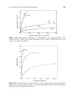
Figure 5.10 Time series, power spectra and distributions of different signals and noises found on
the ECG. From left to right: (1) the underlying electrocardiogram signal, (2) additive (Gaussian)
observation noise, (3) a combination of muscle artifact (MA) and baseline wander (BW), and (4)
power-line interference, sinusoidal noise with f ≈ 33 Hz ±2 Hz.
Figure 5.10 illustrates the time series, power spectra, and distributions of dif-
ferent signals and noises found in an ECG recording. Note that all the signals have
significant power contributions within the frequency of interest (< 40 Hz) where
there exists clinically relevant information in the ECG. Traditional filtering meth-
ods, therefore, cannot remove these noises without severely distorting the underlying
ECG.
5.4.3.4 ICA for Removing Noise on the ECG
For the application of ICA for noise removal from the ECG, there is an added
complication; the sources (that correspond to cardiac sources) have undergone a
context-dependent transformation that depends on the signal within the analysis
window. Therefore, the sources are not clinically relevant ECGs, and the trans-
formation must be inverted (after removing the noise sources) to reconstruct the
clinically meaningful observations. That is, after identifying the sources of interest

we can discard those that we do not want by altering the inverse of the demixing
matrix to have columns of zeros for the unwanted sources, and reprojecting the
P1: Shashi
August 30, 2006 11:5 Chan-Horizon Azuaje˙Book
5.4 Data-Determined Basis Functions 163
data set back from the IC space into the observation space in the following manner:
X
T
filt
= W
−1
p
Y
T
(5.38)
where W
−1
p
is the altered inverse demixing matrix. The resultant data X
filt
is a
filtered version of the original data X.
The sources that we discover with PCA have a specific ordering according to the
energy along each axis for a particular source. This is because we look for the axis
along which the data vector has maximum variance, and, hence, energy or power.
25
If the SNR is large enough, the signal of interest is confined to the first few com-
ponents. However, ICA allows us to discover sources by measuring a relative cost
function between the sources that is dimensionless. Therefore, there is no relevance
to the order of the columns in the separated data, and often we have to apply further

signal-specific measures, or heuristics, to determine which sources are interesting.
Any projection onto another set of axes (or into another space) is essentially a
method for separating data out into separate components, or sources, which will
hopefully allow us to see important structure in a particular projection. For example,
by calculating the power spectrum of a segment of data, we hope to see peaks at
certain frequencies. Thus, the power (amplitude squared) along certain frequency
vectors is high, meaning we have a strong component in the signal at that frequency.
By discarding the projections that correspond to the unwanted sources (such as the
noise or artifact sources) and inverting the transformation, we effectively perform
a filtering of the signal. This is true for both ICA and PCA, as well as Fourier-based
techniques. However, one important difference between these techniques is that
Fourier techniques assume that the projections onto each frequency component are
independent of the other frequency components. In PCA and ICA, we attempt to
find a set of axes that are independent of one another in some sense. We assume
there are a set of independent sources in the data set, but do not assume their
exact properties. Therefore, in contrast to Fourier techniques, they may overlap in
the frequency domain. We then define some measure of independence to facilitate
the decorrelation between the assumed sources in the data set. This is done by
maximizing this independence measure between projections onto each axis of the
new space into which we have transformed the data set. The sources are the data
set projected onto each of the new axes.
Figure 5.11 illustrates the effectiveness of ICA in removing artifacts from the
ECG. Here we see 10 seconds of three leads of ECG before and after ICA decompo-
sition (upper and lower graphs, respectively). Note that ICA has separated out the
observed signals into three specific sources: (1) the ECG, (2) high kurtosis transient
(movement) artifacts, and (3) low kurtosis continuous (observation) noise. In par-
ticular, ICA has separated out the in-band QRS-like spikes that occurred at 2.6 and
5.1 seconds. Furthermore, time-coincident artifacts at 1.6 seconds that distorted the
QRS complex were extracted, leaving the underlying morphology intact.
Relating this back to the cocktail party problem, we have three “speakers” in

three locations. First and foremost, we have the series of cardiac depolarization/
25.
All the projections are proportional to x
2
.
P1: Shashi
August 30, 2006 11:5 Chan-Horizon Azuaje˙Book
164 Linear Filtering Methods
Figure 5.11 Ten seconds of three-channel ECG: (a) before ICA decomposition and (b) after ICA de-
composition. Note that ICA has separated out the observed signals into three specific sources: (1) the
ECG, (2) high kurtosis transient (movement) artifacts, and (3) low kurtosis continuous (observation)
noise.
repolarization events corresponding to each heartbeat, located in the chest. Each
electrode is roughly equidistant from each of these. Note that the amplitude of the
third lead is lower than the other two, illustrating how the cardiac activity in the
heart is not spherically symmetrical. Another source (or speaker) is the perturbation
of the contact electrode due to physical movement. The third speaker is the Johnson
(thermal) observation noise.
However, we should not assume that ICA is a panacea to remove all noise.
In most situations, complications due to lead position, a low SNR, and positional
changes in the sources cause serious problems. The next section addresses many
of the problems in employing ICA, using the ECG as a practical illustrative guide.
Moreover, since an ICA decomposition does not necessarily mean the relevant clini-
cal characteristics of the ECG have been preserved (since our interpretive knowledge
of the ECG is based upon the observations, not the sources). In order to reconstruct
the original ECGs in the absence of noise, we must set to zero the columns of the
demixing matrix that correspond to artifacts or noise, then invert it and multiply
by the decomposed data set to “restore” the original ECG observations.
An example of this procedure using the data set in Figure 5.11 is presented
in Figure 5.12. In terms of our general ICA formalism, the estimated sources

ˆ
Z [Figure 5.11(b)] are recovered from the observation X [Figure 5.11(a)] by esti-
mating a de-mixing matrix W. It is no longer obvious to which lead the underlying
source [signal 1 in Figure 5.11(b)] corresponds. In fact, this source does not cor-
respond to any clinical lead, just some transformed combination of leads. In order
to perform a diagnosis on this lead, the source must be projected back into the
observation domain by inverting the demixing matrix W. It is at this point that we
can perform a removal of the noise sources. Columns of W
−1
that correspond to
noise and/or artifact [signal 2 and signal 3 on Figure 5.11(b) in this case] are set to
P1: Shashi
August 30, 2006 11:5 Chan-Horizon Azuaje˙Book
5.4 Data-Determined Basis Functions 165
Figure 5.12 Ten seconds of data after ICA decomposition (see Figure 5.11), and reconstruction
with noise channels set to zero.
zero (W
−1
→ W
−1
p
) where the number of nonnoise sources is p = 1. The filtered
version of each clinical lead of X is then reconstructed in the observation domain
using (5.38) to reveal a cleaner three-lead ECG (Figure 5.12).
5.4.3.5 Practical Problems with ICA
There are two well-known issues with standard ICA which makes filtering prob-
lematic. Since we can premultiply the mixing matrix A by any other matrix with
the same properties, we can arbitrarily scale and permute the filtered output, Y.
The scaling problem is overcome by inverting the transformation (after setting the
relevant columns of W

−1
to zero). However, the permutation problem is a little
more complicated since we need to apply a set of heuristics to determine which
ICs are signal and which are noise. (Systems to automatically select such channels
are not common and are specific to the type of signal and noise being analyzed.
He et al. [41] devised a system to automatically select channels using a technique
based upon kurtosis and variance.) However, caution in the use of ICA is advised,
since the linear stationary mixing paradigm does not always hold, even approx-
imately. This is because the noise sources tend to originate from relatively static
locations (such as muscles or the electrodes) while the cardiac source is rotating
and translating through the abdomen with respiration. For certain electrode place-
ments and respiratory activity, the ICA paradigm holds, and demixing is possible.
However, in many instances the assumptions break down, and a method for track-
ing the changes in the mixing matrix is needed. Possibilities include the Kalman
filter, hidden Markov models, or particle filter–based formulations [42–44].
To summarize, a useful ICA-based ECG filtering algorithm must be able to:
•
Track nonstationarities in the mixing between signal and noise sources;
•
Separate noise sources from signals for the given set of ECG leads;
•
Identify which ICs are signal related and which ICs are noise related;
•
Remove the ICs corresponding to noise and invert the transformation without
causing significant clinical distortion in the ECG.
26
Even if a robust ICA-based algorithm for tracking the nonstationarities in the
ECG signal-noise mixing is developed, it is unclear whether it is possible to develop
26.
“Clinical distortion” refers to any distortion of the ECG that leads to a significant change in the clinical

features (such as QT interval and ST level).
P1: Shashi
September 4, 2006 10:37 Chan-Horizon Azuaje˙Book
166 Linear Filtering Methods
a robust system to distinguish between the ICs and identify which are noise related.
Furthermore, since the ICA mixing/demixing matrix must be tracked over time,
the filter response is constantly evolving, and thus, it is unclear if ICA will lead
to significant distortions in the derived clinical parameters from the ECG. Other
problems include the possibility that the noise sources can sometimes be correlated
to the cardiac source (such as for drug injections that change the dynamics of the
heart and simultaneously agitate the patient causing electrode noise). Finally, the
lack of high quality data in more than one or two leads can severely restrict the
effectiveness of ICA.
There is, however, an interesting connection between ICA and wavelet analysis.
In restricted circumstances (two-dimensional image analysis) ICA can be shown
to produce Gabor wavelet-like basis functions [45]. The use of ICA as a post-
processing step after construction of a scalogram or spectrogram may provide a
more effective way of identifying interesting components in the signal. Furthermore,
wavelet basis functions do not necessarily have to be orthogonal and therefore offer
more flexibility in separating correlated, yet independent, transient sources.
5.4.3.6 Measuring Clinical Distortion in Signals
Although a variety of filtering techniques have been presented in this chapter, no
method for systematically analyzing the effect of a filter on the ECG has been
described. Unfortunately, simple measures based on RMS error and similar metrics
do not tell us how badly a technique distorts the ECG in terms of the useful clinical
metrics (such as the QT interval and the ST level). In order to do this, a sensitivity
analysis to calibrate the evaluation metric against each clinical parameter is required.
Furthermore, since simple mean square error-based metrics such as those presented
above can give different values for equal power signals with different colorations
(or autocorrelations), it is important to perform a separate analysis of the signal

over a wide range of correlated noises. This, of course, presents another question:
how may we measure the coloration of the noise in the ECG?
One approach to this problem is to pass a QRS detector across the ECG, align
all the beats in the window (ensuring it is large enough, say, 60 beats), and perform
SVD using only the first five components (which encode all the information and
very little noise). If we then calculate the residual (the reconstructed signal minus
the observation) and plot the spectrum of this signal, we will observe a 1/ f
β
-like
slope in the log −log plot. Performing a regression on this line gives us our value
of β, which corresponds to the the color of the noise. (β = 0 is white noise, β =
1 is pink nose, β = 2 is brown noise, and β>2 is black noise.) See [46] for
more details of this method. It should be noted, however, that simple colored noise
models may be insufficient to capture the nonstationary nature of many noises,
and an autoregressive moving average model (ARMA) may be more appropriate
for categorizing noise types. This, of course, is a more complex and less intuitive
approach.
If we have calculated the performance of a filter in terms of the distortion of a
clinical parameter as a function of SNR and color, then this SVD-based and least-
squares fitting method allows us to know exactly the form of the error surface in the
power-color plane. Therefore, we can assess how likely our chosen filtering method
P1: Shashi
August 30, 2006 11:5 Chan-Horizon Azuaje˙Book
5.5 Summary and Conclusions 167
is causing a clinically significant amount of distortion. If different filters lead to large
difference in the distortion levels for different colors and/or SNRs, then a mechanism
for switching between filters may help optimize filtering performance and minimize
clinical distortion. Furthermore, we are able to obtain a beat-by-beat evaluation
of whether we should trust the filtered signal in a particular circumstance. The
derivation of confidence limits on the output of an algorithm for a particular signal

are extremely important, and this concept will be discussed further in Chapter 11.
5.5 Summary and Conclusions
Linear filtering has been presented from the generalized viewpoint of matrix trans-
formations to project observations into a new subspace whose axes are either a
priori defined (as in Fourier-like decompositions) or discovered from the structure
of the observations themselves. The new projections hopefully reveal different un-
derlying sources of information in the observations. The sources are then correlated
with either the signal or the noise. If the subspace dimensionality is less than the
original observation space, then the matrix transformation is lossy.
If the sources are discovered from the structure of the data, it is possible to
separate sources, which may overlap in the frequency domain. It has been shown
that the method for discovering this type of subspace can be cast in terms of a
neural network learning paradigm where the difference between the axes depends
on the activation function and the cost function used in the error back propaga-
tion update. If the underlying sources are assumed to have Gaussian PDFs, then a
linear activation function should be used. Nonlinear activation functions should be
used for non-Gaussian sources. (A tanh function, for example, implies heavy tailed
latent variables.) Additionally, the use of a mean-square error cost function pro-
vides second-order decorrelation and leads to orthogonal basis functions. A mutual
information-based cost function performs a fourth-order decorrelation and leads to
a set of nonorthogonal basis functions. By projecting the observations onto these ba-
sis functions, using the discovered demixing matrix to provide the transformation,
the estimated source signals are revealed.
To improve the robustness of the separation of partially or completely unknown
underlying sources, either a statistically constructed model (as with learning algo-
rithms in this chapter), or an explicit parameterized model of the ECG can be used.
However, since the ECG is obviously nonlinear and nonstationary, the chosen signal
processing technique must be appropriately adapted. Nonlinear ECG model-based
techniques are therefore presented in the next chapter, together with an overview
of how to apply nonlinear systems theory and common pitfalls encountered with

such techniques.
References
[1] S
¨
ornmo, L., and P. Laguna, Bioelectric Signal Processing in Cardiac and Neurological
Applications, Amsterdam: Elsevier (Academic Press), 2005.
[2] Rangayyan, R. M., Biomedical Signal Analysis: A Case-Study Approach, Series on
Biomedical Engineering, New york: Wiley-IEEE Press, 2002.
P1: Shashi
August 30, 2006 11:5 Chan-Horizon Azuaje˙Book
168 Linear Filtering Methods
[3] Cohen, R., and A. Ryan, Wavelets and Multiscale Signal Processing, London, U.K.:
Chapman and Hall, 1995.
[4] Williams, W., “Recent Advances in Time-Frequency Representations: Some Theoreti-
cal Foundation,” in M. Akay, (ed.), Time Frequency and Wavelets in Biomedical Signal
Processing, Chapter 1, New York: Wiley-IEEE Press, 1997.
[5] Addison, P. S., “Wavelet Transforms and the ECG: A Review,” PhysiologicalMeasurement,
Vol. 26, No. 5, 2005, pp. R155–R199.
[6] Dickhaus, H., and H. Heinrich, “Analysis of ECG Late Potentials Using Time-Frequency
Methods,” in M. Akay, (ed.), Time Frequency and Wavelets in Biomedical Signal Process-
ing, Chapter 4, New York: Wiley-IEEE Press, 1997.
[7] Mart´ınez, J. P., et al., “A Wavelet-Based ECG Delineator: Evaluation on Standard
Database,” IEEE Trans. Biomed. Eng., Vol. 51, No. 4, 2004, pp. 570–581.
[8] Laguna, P., 2006.
[9] Grinfeld, P., “The Gibbs Pheonomenon — Java Applet Demo,” 1999, h.
drexel.edu/∼pg/fb//java/la
applets/Gibbs/index.html.
[10] Greenberg, J., HST.582J/6.555J/16.456J, “Design of FIR Filters by Windowing,” 1999,
/>[11] Antoniadis, A., and J. Fan, “Regularization of Wavelet Approximations,” Journal of the
American Statistical Association, Vol. 96, No. 455, 2001, pp. 939–967.

[12] Hilton, M. F., et al., “Evaluation of Frequency and Time-Frequency Spectral Analysis of
Heart Rate Variability as a Diagnostic Marker of the Sleep Apnoea Syndrome,” Med. Biol.
Eng. Comput., Vol. 37, No. 6, November 1999, pp. 760–769.
[13] Huang, N. E., et al., “The Empirical Mode Decomposition and the Hilbert Spectrum for
Nonlinear and Non-Stationary Time Series Analysis,” Proc. R. Soc. Lond. A, Vol. 454,
1998, pp. 903–995.
[14] Huang, N. E., and S. S. Shen, The Hilbert-Huang Transform and Its Applications,
Singapore: World Scientific Publishing Company, 2005, />mathematics/etextbook/5862/.
[15] Golub, G. H., and C. F. Van Loan, Matrix Computations, 2nd ed., Oxford, U.K.: North
Oxford Academic, 1989.
[16] Moody, G. B., and R. G. Mark, “QRS Morphology Representation and Noise Estimation
Using the Karhunen-Lo
`
eve Transform,” Computers in Cardiology, 1989, pp. 269–272.
[17] Mark, R. G., and G. B. Moody, “ECG Arrhythmia Analysis: Design and Evaluation Strate-
gies,” Chapter 18 in I. Gath and G. F. Inbar, (eds.), Advances in Processing and Pattern
Analysis of Biological Signals, New York: Plenum Press, 1996, pp. 251–272.
[18] Clifford, G. D., and L. Tarassenko, “One-Pass Training of Optimal Architecture Auto-
Associative Neural Network for Detecting Ectopic Beats,” IEE Electronic Letters, Vol.
37, No. 18, August 2001, pp. 1126–1127.
[19] Gao, D., et al., “Bayesian ANN Classifier for ECG Arrhythmia Diagnostic System: A
Comparison Study,” International Joint Conference on Neural Networks, Montreal, July
2005.
[20] Bishop, C., Neural Networks for Pattern Recognition, New York: Oxford University Press,
1995.
[21] Clifford, G. D., L. Tarassenko, and N. Townsend, “Fusing Conventional ECG QRS De-
tection Algorithms with an Auto-Associative Neural Network for the Detection of Ectopic
Beats,” 5th International Conference on Signal Processing, Beijing, China, August 2000,
IFIP, World Computer Congress, pp. 1623–1628.
[22] Tarassenko, L., G. D. Clifford, and N. Townsend, “Detection of Ectopic Beats in the Elec-

trocardiogram Using an Auto-Associative Neural Network,” Neural Processing Letters,
Vol. 14, No. 1, 2001, pp. 15–25.
[23] Golub, G. H., “Least Squares, Singular Values and Matrix Approximations,” Applikace
Matematiky, No. 13, 1968, pp. 44–51.
P1: Shashi
August 30, 2006 11:5 Chan-Horizon Azuaje˙Book
5.5 Summary and Conclusions 169
[24] Bourlard, H., and Y. Kamp, “Auto-Association by Multilayer Perceptrons and Singular
Value Decomposition,” Biol. Cybern., No. 59, 1988, pp. 291–294.
[25] Bunch, J. R., and C. P. Nielsen, “Updating the Singular Value Decomposition,” Numer.
Math., No. 31, 1978, pp. 111–129.
[26] Tarassenko, L., A Guide to Neural Computing Applications, Oxford, U.K.: Oxford
University Press, 1998.
[27] MacKay, D. J. C., “Maximum Likelihood and Covariant Algorithms for Independent
Component Analysis,” />1996, updated 2002.
[28] Clifford, G. D., 2003, updated June 2006.
[29] Greenberg, J., et al., HST.582J/6.555J/16.456J, “Biomedical Signal and Image Processing:
Course Notes,” 2006.
[30] Trotter, H. F., “An Elementary Proof of the Central Limit Theorem,” Arch. Math., Vol. 10,
1959, pp. 226–234.
[31] Penny, W., S. Roberts, and R. Everson, “ICA: Model Order Selection and Dynamic
Source Models,” Chapter 12 in S. Roberts and R. Everson, (eds.), Independent Com-
ponent Analysis: Principles and Practice, Cambridge, U.K.: Cambridge University Press,
2001.
[32] Choudrey, R. A., and S. J. Roberts, “Bayesian ICA with Hidden Markov Model Sources,”
International Conference on Independent Component Analysis, Nara, Japan, 2003,
pp. 809–814.
[33] Joho, M., H. Mathis, and R. Lambert, “Overdetermined Blind Source Separation: Using
More Sensors than Source Signals in a Noisy Mixture,” Proc. International Conference
on Independent Component Analysis and Blind Signal Separation, Helsinki, Finland, June

19–22, 2000, pp. 81–86.
[34] Lee, T., et al., “Blind Source Separation of More Sources than Mixtures Using Overcom-
plete Representations,” IEEE Sig. Proc. Lett., Vol. 6, No. 4, 1999, pp. 87–90.
[35] Lewicki, M. S., and T. J. Sejnowski, “Learning Overcomplete Representations,” Neural
Computation, Vol. 12, No. 2, 2000, pp. 337–365.
[36] Benaroya, L., et al., “Non Negative Sparse Representation for Wiener Based Source,”
Proc. ICASSP, Hong Kong, 2003, pp. 613–616.
[37] Clifford, G. D., and P. E. McSharry, “A Realistic Coupled Nonlinear Artificial ECG, BP,
and Respiratory Signal Generator for Assessing Noise Performance of Biomedical Signal
Processing Algorithms,” Proc. of SPIE International Symposium on Fluctuations and
Noise, Vol. 5467, No. 34, 2004, pp. 290–301.
[38] McSharry, P. E., and G. D. Clifford, “A Comparison of Nonlinear Noise Reduction and
Independent Component Analysis Using a Realistic Dynamical Model of the Electrocar-
diogram,” Proc. of SPIE International Symposium on Fluctuations and Noise, Vol. 5467,
No. 9, 2004, pp. 78–88.
[39] James, C. J., and D. Lowe, “Extracting Multisource Brain Activity from a Single Elec-
tromagnetic Channel,” Artificial Intelligence in Medicine, Vol. 28, No. 1, May 2003,
pp. 89–104.
[40] Broomhead, D. S., and G. P. King, “Extracting Qualitative Dynamics from Experimental
Data,” Physica D, Vol. 20, 1986, pp. 217–236.
[41] He, T., G. D. Clifford, and L. Tarassenko, “Application of ICA in Removing
Artifacts from the ECG,” Neural Comput. and Applic., Vol. 15, No. 2, 2006, pp. 105–
116.
[42] Penny, W., S. Roberts, and R. Everson, “Hidden Markov Independent Components Analy-
sis,” Chapter 1 in M. Grolami, (ed.), Advances in Independent Component Analysis, New
York: Springer-Verlag, 2000.
[43] Penny, W., S. Roberts, and R. Everson, “Hidden Markov Independent Components for
Biosignal Analysis,” Proc. of MEDSIP-2000, 2000.