Maya Secrets of the Pros Second Edition phần 8 pptx

The next steps take us through creating the dynamics for this surface:
1. Select the plane, and (in the Dynamics menu set) choose Soft/Rigid Bodies → Create
Soft Body ❒.
2. In the option box, set Creation Options to Duplicate, Make Copy Soft, check Hide
Non-Soft Object, and turn on Make Non-Soft a Goal. Click Create to make the soft
body surface.
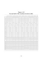
3. Maya will create a grid of particles that correspond to the location of the CVs on
that plane. Figure 7.30 shows the particles with the plane turned off. As a matter
of fact, go into the persp panel’s menu (choose Show → NURBS Surfaces) to toggle
its display off; we’ll just deal with the grid of particles for right now. The file
rain_puddle_soft_body_start.ma on the CD contains the plane turned into the
proper soft body object and will bring you up to this point in the exercise.
Now, we’ll make a quick collision object to see how the particles move.
4. Create a polygonal sphere, and place it above the particle grid, as shown in Fig-
ure 7.31.
5. Select the sphere and turn it into an active rigid body with a gravity field on it by
choosing Soft/Rigid Bodies → Create Active Rigid Body, and then, with the sphere still
selected, choose Fields → Gravity.
Of course, you can do this a bit quicker by just selecting the sphere and creating the grav-
ity field. Maya automatically turns the sphere into an active rigid body and connects the
gravity to it.
■ Raining Cats and Dogs 195
Figure 7.30: The grid of particles for the soft body plane Figure 7.31: Place the ball as shown.
4345c07p3.1.qxd 1/1/05 11:05 AM Page 195
6. If you play back the anima-
tion, the sphere falls and
passes through the particles
below it. To make the sphere
collide with the particles,
select the particles, select the
sphere, and choose Particles →

Make Collide.
7. Now if you play back the
animation, you’ll more than
likely see the particles not
react in the slightest as the
sphere passes through them
again. This is because the
particles still have their goal
weight set to 1. Now we
don’t need to set per particle
goal weights on the water
surface, so select the particles
and in the Attribute Editor, in
the Goal Weights and
Objects section, turn the nurbsPlaneShape1 weight down to 0.5 for now.
8. If you play back the animation, you’ll see the particles getting pushed through the grid
and bounce back up and down until they settle back into the grid. You may have to
increase your playback range to see all this, though. Figure 7.32 shows the particles
(colored yellow here) that are being pushed through the grid by the sphere.
Using Springs to Create Ripples
The goal object of the plane makes the particles bounce back into place, but there are no rip-
ples in the surface. This is simply because the movement of one particle does not affect the
movement of the others. The goal object merely pulls the out-of-place particles back to their
original location at their respective CV. Creating ripples calls for the use of springs.
Soft Body dynamic springs connect individual particles of the same particle object
together in a few ways. Follow these steps to add springs to the water surface:
1. Select the particle object, and choose Soft/Rigid Bodies → Create Springs ❒.
2. In the option box, give the springs a name if you want. Then change Creation Method
to Wireframe. This creation method will make springs that attach from particle to par-
ticle. Leave Wire Walk Length at 1 (or change it if yours is different). Wire Walk

Length specifies how many particles over in all directions to the current particle the
spring will be created. With a length of 1, only the immediately adjacent particles will
be connected with springs.
Springs can be taxing on a computer when you run the simulation, so use the least num-
ber of springs you can get away with for the simulation to work properly.
196 chapter 7 ■ A Dynamics Collection: Flexible Objects
Figure 7.32: The yellow particles shown here are being
pushed through by the colliding sphere.
4345c07p3.1.qxd 1/1/05 11:05 AM Page 196
3. Figure 7.33 shows all the creation options for
the springs we want to create. Once you match
these settings, click Create to make the springs.
You should now see dashed lines (the springs)
connecting the individual particles, as shown in
Figure 7.34.
4. If you play back the animation, you’ll see a
small amount of ripple go through as the sphere
pushes through the grid. We’ll need more of a
ripple, though, since the ripple doesn’t really go
far from the impact. Select the springs we just
made, and change Stiffness to a high number
such as 64. This will help pull the adjacent
particles into the fray.
5. Also, you can decrease the goal weight for the
particles to about 0.3 instead of your current
0.5. Select the particle object, open the Attribute
Editor, and decrease the nurbsPlaneShape1
weight to 0.3. This should give you a nice ripple,
as shown in Figure 7.35.
If you find your computer is sluggish during this exercise, you can by all means use a less

subdivided NURBS plane instead of our 100-by-100 subdivided plane. This will decrease
the computing power you’ll need.
■ Raining Cats and Dogs 197
Figure 7.33: The options for creating springs Figure 7.34: The springs
Figure 7.35: A ripple cascades in the softbody surface.
4345c07p3.1.qxd 1/1/05 11:05 AM Page 197
This simulation is useful for making a rock hit the surface of a pond, but now let’s
make rain drops. We may find that with the number of raindrops that fall, we may have to
go back in and adjust our spring and goal weight settings so that that puddle’s surface does
not go too crazy with deformation.
Making Rain
It would not be prudent to create hundreds of little active body spheres that fall onto the
pond. Instead, we will use particles to rain down on our water surface. To create the particles,
follow these steps:
1. Delete the sphere from the scene as well as its gravity field. Create a volume emitter in
the shape of a cube, and size/place it above the surface, as shown in Figure 7.36. To
create the emitter, choose Particles → Create Emitter ❒. In the option box, set Emitter
Type to Volume, set Rate at 50, and make sure Volume Shape is set to Cube. In the Vol-
ume Speed Attributes section, set Away From Center to 0, set Along Axis to –1, and set
all the other options to 0, as shown in Figure 7.37.
2. If you run the simulation, you’ll see particles slowly trickling out of the emitter. Select
this new particle object, and add gravity to it by choosing Fields → Gravity. Select the
gravity, and change Magnitude to 20. This will help pull the particles down. Figure
7.38 shows the particle rain.
Now the task becomes getting the particles to collide with the water surface. But this is
more complicated than selecting the water surface plane and the particles and choosing Par-
ticles → Make Collide as we did with the falling sphere and the particles. Doing that will just
make the particle rain bounce off the top of the surface. We need to make the rain particles
collide with and move the surface’s particles to get the surface to deform. But here’s the
caveat: particles cannot collide with other particles. The best solution is to create fields that

will move the surface particles instead of a collision. To do that, follow these steps.
3. Select the surface particles, and choose Fields → Radial to connect a radial field to the
deforming particles.
198 chapter 7 ■ A Dynamics Collection: Flexible Objects
Figure 7.36:
Place a cube vol-
ume emitter
above the grid to
make the rain.
4345c07p3.1.qxd 1/1/05 11:05 AM Page 198
4. We need the rain particles to be the
source of the radial field. Select the
radial, and then select the rain parti-
cles. Choose Fields → Use Selected As
Source of Field. If you play back the
simulation now, the rain will begin
pushing the entire surface down and
warp it, as opposed to creating inden-
tations for each of the rain particles as
they pass through the water surface
(see Figure 7.39).
5. Select the radial field, which is now
grouped under the rain particle node, and in the Channel box, change Apply per Ver-
tex to On. You’ll now see the particles really warping the surface, as in Figure 7.40.
6. Select the radial field and decrease Max Distance to a lower number such as 2. This
will make the radial field ineffectual until the individual particles are within 2 units
■ Raining Cats and Dogs 199
Figure 7.37: The Emitter Options (Create)
dialog box
Figure 7.38: It’s raining pixels!

Figure 7.39: The rain particles are acting as a whole to
deform the entire soft body surface.
4345c07p3.1.qxd 1/1/05 11:05 AM Page 199
from the surface particles. You can then play with the magnitude of the radial field to
dial in the amount of surface disruption you want from the drops. Figure 7.41 shows
the radial field’s effect with Max Distance set to 2 and Magnitude set to 10.
Adding Splashes
The next task is adding splashes to each of the rain particles as they hit the puddle’s surface.
This fairly simple process involves particle collisions. Follow these steps:
1. Create a new NURBS plane, and scale it up to fit the current puddle surface area. Place
it just below the puddle surface. This will be the collision surface to generate the new
splash particles.
2. Select the rain particles, and then select the new plane. Choose Particles → Make Col-
lide. Select the new plane and template it so that it does not render and is out of the
way. The intent here is that the rain fall through the puddle surface, cause ripples, and
then immediately hit the essentially invisible plane right underneath, creating a colli-
sion. If you play back the simulation now, you’ll just see the particles bouncing up, as
in Figure 7.42.
3. With the rain particles selected, choose Particles → Particle Collision Events. In the
window, make sure the right particle system (particle1) is selected in the Objects win-
dow. For Type, check Split, and change Num particles to 10. Click Create Event.
4. A new particle system node is created (particle2). Select it in the Outliner, and open the
Dynamic Relationships window (choose Window → Relationship Editors → Dynamic
Relationships. With particle2 selected in the left column, select the gravity field we
have on the rain particles (gravityField2).
200 chapter 7 ■ A Dynamics Collection: Flexible Objects
Figure 7.40: The rain particles are more than ever warping
the entire surface.
Figure 7.41: The puddle is pelted by rain.
4345c07p3.1.qxd 1/1/05 11:05 AM Page 200

5. Open the Attribute Editor for the new splash particles, set their Lifespan Mode to Ran-
dom Range, set Lifespan to 2.5, and set Lifespan Random to 0.5. Play back the simula-
tion to see something like Figure 7.43.
The Ring
Now we’ll take a quick look at how to kick up dust for a rolling object such as an inner tube.
Following in the same vein as the previous exercise on creating rain splashes in a pond, we’ll
use collisions to create new particles from our ground plane. An effect such as this is tremen-
dously useful for creating a sense of impact when an object travels (rolls, slides, bounces, and
so on) along a path such as a dirt road, snow, or the like.
In theory, the exercise is fairly straightforward; we’ll use an object (the inner tube) to
interact with the ground to generate a particle dust. The setup begins with making the geom-
etry and turning the geometry into dynamic objects. You then give the scene dynamic forces
to create motion and to define collisions between bodies and particles. To accentuate the
effect, the collisions generate a new particle system to make the dust flare up and out from
the impact.
To set up the scene, follow these steps:
1. Create a ground plane for the collision detection and for our inner tube to roll on.
Increase the subdivisions to gain a well-tessellated plane.
2. Create a polygonal torus for the inner tube, increase its subdivision axis to 30, and set
its shape and location as shown in Figure 7.44. Notice it is placed a few units above the
ground plane to give it an initial bouncing.
■ The Ring 201
Figure 7.42: The rain particles will now bounce back up
off the collision plane right under the water’s surface plane
as it ripples.
Figure 7.43: The splashes shown in white are created when
the blue rain particles hit the collision surface below the
water surface.
4345c07p3.1.qxd 1/1/05 11:05 AM Page 201
3. Now, we should create collisions for the tube and ground. Select the plane, and make

it into a passive rigid body by choosing Soft/Rigid Bodies → Create Passive Rigid
Body →❒. In the option box, reestablish the settings before you invoke the action.
4. Select the tube, and choose Soft/Rigid Bodies → Create Active Rigid Body →❒. In the
option box, reestablish the settings (just in case something is different from the
defaults) and create the Active Rigid Body.
5. Select the tube, and add a gravity field to it by choosing Fields → Gravity.
If you play back the simulation, you’ll notice the tube falls, bounces on the ground,
and may fall over on its side. As we would with a bike, we’ll have to give the tube some spin
to get it rolling on the ground. While we’re at it, let’s add some momentum to it as well. To
do so, follow these steps:
1. Select the active rigid body torus, and in the Channel box, change Initial Spin Y to 400.
This gives the torus a bit of a spin, but only at the beginning of simulation. When you
play back the scene, you’ll notice the tube has some momentum to roll forward when it
hits the ground.
2. Add a bit more momentum to the tube by selecting the torus and changing the Initial
Velocity X attribute to –3. If you play back the simulation, you’ll see the tube lurch
into motion a bit more, bounce a few times on the ground, and slowly roll off the far
edge of the plane. Figure 7.45 shows the tube making its first bounce. Depending on
how your scene is oriented, you may need to use Initial Velocity Z or Y instead of X to
get it moving in the right direction.
The setup for making dust kick up with particles is similar to the earlier puddle setup.
Particles on the surface of the ground (like the soft body particles of the pond surface) will
202 chapter 7 ■ A Dynamics Collection: Flexible Objects
Figure 7.44:
Place the inner
tube above the
ground plane.
4345c07p3.1.qxd 1/1/05 11:05 AM Page 202
detect collisions with the torus surface and
spawn new particles that will create a dust

hit every time the tube touches the ground.
Consequently, we have to create a field
of particles on the ground plane for the torus
to bounce on and roll through. We can do so
in a few ways. For example, we can use the
Particle tool to create a grid of particles and
simply place it on the plane or just above it.
This is perhaps the easiest way. We will emit
particles from the plane to get a more ran-
dom arrangement than we would with a grid
of particles from the Particle tool.
To set up the dust hits, follow these
steps:
1. Select the plane and choose Particles →
Emit from Object →❒. In the option
box, set Emitter Type to Surface and set Rate to 10000. Set all the Speed attributes to
zero and click Create. Figure 7.46 shows the option box. Setting all Speed attributes
to 0 makes the particles appear on the surface, and they will not travel. The high rate
will come in handy in the next step.
2. Play back the animation, and watch the plane fill with particles. Stop the playback at
about frame 50 or until the plane looks like the one in Figure 7.47.
■ The Ring 203
Figure 7.45:
Bouncy bouncey!
Figure 7.46: The proper options for creating the
ground particles
4345c07p3.1.qxd 1/1/05 11:05 AM Page 203
3. With the particle object
selected, choose Solvers →
Initial State → Set for

Selected. This will display the
particles in this state from the
beginning. Select the emitter
(grouped under the ground
plane) and set Rate back to 0
as in Figure 7.48. This pre-
vents the plane from produc-
ing any more particles; we
have plenty now.
Setting Up the Collision
Detection
Now we need to create the colli-
sion detection that will eventually
spawn the dust hits for us as the
tube touches down and rolls across the ground. Follow along to create the collisions:
1. Select the particle object and the tube, and choose Particles → Make Collide →❒. In
the option box, set Resilience to 0.3. This will keep the particles from flying away
when they get hit by the tube.
204 chapter 7 ■ A Dynamics Collection: Flexible Objects
Figure 7.47: The
particles cover
the ground
plane.
Figure 7.48: Turn off the emission of the particles after you
set the initial state.
4345c07p3.1.qxd 1/1/05 11:05 AM Page 204
2. If you play back the simulation, you’ll notice nothing really happens; the tube bounces
along, and nothing happens to the particles even if they collide with the tube. This is
because the particles need to rest a bit higher in the scene, just above the ground plane
that emitted them. So select the particle object node, and raise it just a tiny bit above

the ground plane, as in Figure 7.49.
3. If you play back the scene, you’ll see some of the particles being hit and flying away, as
shown in Figure 7.50. (The particles get pushed
down.)
4. Now we’ll need to kill some of those particles to
prevent them from bouncing around all over the
scene, and we’ll need them to spawn more parti-
cles to give us the dust effect hit. Choose Parti-
cles → Particle Collision Events to open the Par-
ticle Collision Events window as shown in
Figure 7.51.
5. Set Event Type to Emit, set Num particles to 50,
and set Spread to 0.5. Also check the All Colli-
sions box, and check the Original Particle Dies
box. Set Target Particle to particle2, which cre-
ates a new particle object for the scene.
6. If you play back your scene, you’ll see new parti-
cles being spawned from the collisions with the
grid of particles on the ground plane, as shown
in Figure 7.52.
■ The Ring 205
Figure 7.49: The particle grid placed right above the plane.
Figure 7.50: The particles are being hit by the tube and flying away.
Figure 7.51: The Particle Collision
Events window
4345c07p3.1.qxd 1/1/05 11:05 AM Page 205
Creating Better Dust Hits
The particles are all going down and away and not making convincing hits. We need them to
bounce up and not through the bottom of the ground plane. Easy enough. We’ll make the
new particles collide with the ground plane.

1. Select the new particles (particle2 in the Outliner) and the ground plane, and choose
Particles → Make Collide →❒. Set Resilience to 0.6 to get a nice bounce as in Fig-
ure 7.53.
2. To settle the dust hits, select them and add gravity by choosing Fields → Gravity. The
particles will now fall to the ground plane and act a bit more like dust. Set Gravity to
0.2 or so to get the dust to kick up a bit better. You already have it set up to collide on
the ground
3. You can control how much the new particles slide across the floor (set into motion
from the collision emission) by increasing the friction attribute of the proper geocon-
nector attribute on the ground plane. There is also an entire chain of events that leads
up to a convincing look to the dust as well as plenty of work getting a good movement
Check out
ring_dust.ma on the CD for this scene. You can play around with its current
settings to get a better feel for how the dynamic attributes affect the animation of the scene.
You will begin to see how useful this sort of simulation can be as you work your way
through your Maya lifeline. It’s actually more the method you use than the procedures you
follow. If you take a good long hard look at the animation you’ve just created, it is actually
quite a bit off the mark for a dust hit effect. As a matter of fact, there is quite a bit more to
do to get this dust to look like dust as well as act like dust.
So in a sense, you’ve just been had.
Why You’ve Been Had
When it comes down to it, it’s the guys and gals who can find the ever-so-thin edge of bal-
ance between all these settings and can create from it an interpretation of the physical laws
that move us all. Getting to the end of a tutorial is really the easy part. The best way to col-
lect ability for CGI is to wander through it slowly. Where this tutorial really begins, and the
education earns its merit, is at the end when you’ve set up your scene. Adjusting the settings
206 chapter 7 ■ A Dynamics Collection: Flexible Objects
Figure 7.52:
New particles
are being created

from the colli-
sions with the
grid of particles
on the ground.
4345c07p3.1.qxd 1/1/05 11:05 AM Page 206
and finding better balances after the scene is set up by the end of the lesson, to find an elo-
quent evolution to a nice animation that convinces but also instructs. Imbuing the animation
with your own personality is art in any animation.
A primary issue with students (and even some professionals) is their reluctance to stop
their “learning” before they really jump into a solid task and come up with a well-considered
solution that not only smacks of solution but glows with finesse. A lot of people equate the
quantity of facts and techniques gained in a tutorial or class proportional to gaining a better
education.
I find too often people jump to learning how to do something new that they hardly ever
linger around enough to learn how to do it well. The interest zone has been left behind and
the next neat trick needs be assimilated as if picking up cheap plastic screwdrivers from a
mass retail bin. One tutorial can well be worth a 10-week course in effects and should be
treated as such.
It’s really important to remember to exhaust yourself on finding personality in motion and
learn how to animate.
Always Learning
Dynamics are a good means to an end. They can help you create automated secondary ani-
mation to add to characters or props in your scene that would otherwise take more time
from your busy animators. Although there are a lot of straightforward uses for dynamics,
such as the antenna, it’s always wise to consider as many options as possible to accomplish
the task at hand. This keeps your options open, since some solutions work better in some
instances than others. Dynamics can also be, in sometimes strange ways, like using hair
dynamic follicles to drive secondary motion for a car setup.
In any event, it is wise to consider dynamics as a tool to begin solving a problem. More
often than not, dynamic solutions are frequently used as just a jumping-off point to animate a

scene. For example, dynamic solutions can be converted to keyframes for easy editing and
manipulation. But the power they can offer in creating automation and effects is indeed sweet.
■ Always Learning 207
Figure 7.53:
Kicking up the
dust particles
4345c07p3.1.qxd 1/1/05 11:05 AM Page 207
CHAPTER
eight
4345c08_p3.1.qxd 1/1/05 11:09 AM Page 208
The Art of (Maya) Noise
By Kenneth Ibrahim and John Kundert-Gibbs
One of the amazing aspects of using Maya for
any length of time is uncovering more and more of its amazingly rich
feature set, which allows creative people to generate remarkable effects
and animation in clever, efficient ways. Maya’s built-in Perlin
noise
function is one of those features that people often overlook, but which, in
the right hands, can produce an impressive variety of effects. In this
chapter, we will introduce you to Maya’s
noise function and show you how
to use it to produce animations worthy of big-budget productions. Some
of our examples, in fact, are similar to effects created for big-name movies
released in the past few years. After reading through this chapter, you may
find yourself thinking, “Gee, I know how to do that effect,” the next time
you pop a hit movie into your DVD player.
First, a Little Theory
Nearly all programmers and savvy Maya users are familiar with the venerable random (or
rand) function, which has been used in everything from war planning, to computer games, to
MP3 song shuffling to produce “random” numbers, events, or actions. Using a seed number

(a float or integer value), a
rand function produces results that appear to have no correlation
to one another over a value interval—typically this interval is 0 to 1, –1 to 1 (as float values)
or –32767 to 32767 (as integer values). To expand the range of values, you can multiply,
divide, add to, or subtract from the raw value returned by the function call. Although the
rand function has some great uses, it is not ideal for every situation in which varying values
are required. For one thing, the
rand function produces numbers that are completely dissoci-
ated from one another, which can produce a “popping” effect during animation. For
4345c08_p3.1.qxd 1/1/05 11:09 AM Page 209
another, the rand function can produce high-frequency “clumping” if many results lie close
to one another—a result that can frustrate attempts to produce effective stochastic simula-
tion (see Figure 8.1).
The random function built into many computer programs is actually any one of a collec-
tion of mathematical functions that produce quasirandom rather than truly random num-
bers. A pseudorandom sequence of numbers appears random when you look at a small
sample of the numbers (say, 100 or 10,000 return values); the numbers, however, are
completely determined by the starting value—or seed number—and eventually repeat if
enough “random” values are extracted from the sequence. Although mathematical formu-
las do a good job of pretending to be random, no one has yet devised one that produces
truly random numbers. Thus, flipping a real coin always produces more random results
than writing a “coin flip” program using a pseudorandom number generator.
Fortunately, Maya’s
noise function can produce elegant results even when the basic
rand function fails. There are two important differences between rand and noise. First,
although seemingly random over the long-term, the
noise function is a continuous function
“connected” over short intervals. In other words, moving from one returned value to the
next is usually a short distance; whereas with the
rand function, values can range from the

maximum possible value to the minimum possible with two consecutive outputs. The sec-
ond difference is that the
noise function takes a continuously varying value (often time) as
its input, rather than a single seed number. The
noise function with a constant input (the
number 1, for example) returns a single value when called, rather than a series of values.
Figure 8.2 shows the Graph Editor curves for an object animated by the
rand function ver-
sus an object animated by the
noise function. In addition, since the value noise returns is
210 chapter 8 ■ The Art of (Maya) Noise
Figure 8.1: High-frequency “clumping” produced by Maya’s rand function. (Note the areas circled
in the image.)
4345c08_p3.1.qxd 1/1/05 11:09 AM Page 210
determined by the input value, you can safely render repeatable sequences using the noise
function across multiple machines provided they have the same operating system, which is
useful when you need to batch render.
Maya’s noise function is an implementation of the Perlin noise function, which produces
self-similar randomness over a range of scales by taking the results of a series of random
numbers and smoothly interpolating over them. In essence, Perlin
noise is a way to gener-
ate fractal results: results in which the “image” appears the same on a multitude of scales.
Noise depends on the rate of change of the input value. If you use the
frame variable
rather than the
time variable (with frames increasing 24 times more rapidly than time if
Maya is set to film units), the resultant motion looks much more random because the
noise
function varies far more rapidly over time. This is because we’re sampling the continuous
noise field at greater intervals, thus returning fewer related values at each step.

As a continuous-but-random sequence, the results of using the
noise function can help
create any number of effects. Creating a realistically varied fountain of water, our first example,
is straightforward to implement using the
noise function to vary the velocity, spread, and rate
of a particle emitter. In addition to using the MEL script command
noise, Maya implements
noise in a variety of other areas, including in procedural texture mapping (the fractal texture,
and the noise feature on several other textures) and in fluid effects to produce effects such as
clouds and smoke. For an artist using Maya, the trick is to “see” noise in patterns and move-
ment around you. Once you see noise in natural phenomena, you’re just a few steps from
implementing it in Maya. For example, the next time you drink from a water fountain, notice
■ First, a Little Theory 211
Figure 8.2: An
animation curve
produced by the
rand function
(top) and the
noise function
(bottom)
4345c08_p3.1.qxd 1/1/05 11:09 AM Page 211
the motion of the water and all those slight variations of pressure and arc in the water. Using a
method similar to our first example, you can re-create these phenomena in Maya.
Now that you have a basic understanding of the
noise function, let’s see how to use it
to create a number of compelling effects in Maya.
Building a Variable-Speed Fountain of Water
To start, let’s use noise to help generate a volume of water rising from a fountain—an effect
that could be used to make the background in a scene more interesting and lively, for example.
Although noise is simple to add to the fountain we create, its addition adds subtle realism and

interest to the animation, making it more interesting than an unmodified particle emitter.
1. Open a new scene in Maya, create a “water” plane on the ground, and scale it out large.
(This plane has nothing to do with the effect. It just helps locate the pool of water.)
2. Create a particle emitter, using the following settings. (Feel free to alter them to suit
your taste.)
Emitter Type: Volume
Volume Shape: Cone
Rate: 2000
Particle Color R, G, and B: Around 0.5
Away from Center: 0
Around Axis: 0
Away from Axis: 1
Along Axis: 20
3. Scale the cone volume shape to something similar to that in Figure 8.3. (In the figure,
the cone was scaled to 0.8, 1.2, and 0.7 in X, Y, and Z. Scaling the cone a bit shapes
the way the particles are emitted from the volume shape. The Away from Axis setting
controls particle speed horizontally (away from the cone’s primary axis), and Along
Axis controls the speed vertically (up the cone’s axis).
4. Play the animation forward some frames, and select the particles. With particles
selected, choose Fields → Gravity (using default settings). The particles should now rise
into the air and then fall back through the plane. To reduce the number of particles
Maya has to keep up with, select the particles again and set Lifespan to 4 (seconds).
You can make this lifespan random too if you like, but as the particles will lie under the
plane before dying, this step is not really necessary.
212 chapter 8 ■ The Art of (Maya) Noise
Figure 8.3: The
volume emitter
cone and ground
plane
4345c08_p3.1.qxd 1/1/05 11:09 AM Page 212

Now we want to use the noise function to vary the emitter’s Away from Axis and
Along Axis settings to create a varying flow rate for the fountain.
5. With the emitter selected, right-click the Away from Axis text, and choose Expressions.
In the Expression Editor, type the following expression:
emitter1.awayFromAxis = 2.0 * noise (time * 4.0);
6. Right-click the Along Axis text, choose Expressions, and type the following equation:
emitter1.alongAxis = 3.0 * (noise (time * 3.0)) + 20.0;
These two simple expressions control the speed of particles in both the horizontal and
vertical directions for the emitter. For the first expression, the
noise function uses 4 times the
value of time (which increments
1
⁄24th of a second for each frame, assuming film settings are
used) to produce an output value between –1 and 1. This number is then multiplied by 2,
generating a final number that lies between –2 and 2 for each frame.
The second expression is only slightly more complex. Here 3 times
time is used as the
input for
noise. (This makes the noise function fluctuate a bit less rapidly than in the previ-
ous algorithm.) The output of this is multiplied by 3—producing a value between –3 and 3—
and this value is added to 20 (the starting speed), thus producing a number between 17 and
23 as the speed along the cone’s axis. The results of these two expressions, shown in Figure
8.4, produce a constantly varying rate of speed in particle emission, as well as a fluctuation
in how widely the particles are dispersed. If you want, you can vary the rate as well using a
similar expression to control the emitter’s rate attribute.
With this animation as a base, you can do a bit of tweaking to get fairly nice looking
results in a minimum of time. By switching the particles to a blobby surface render type,
putting a nearly transparent anisotropic shader on them, and sticking an ocean shader
on the ground plane beneath, the particle fountain can end up looking like Figure 8.5.
Because the

noise function is time-based here, we included an animation of this fountain
on the CD (
noisyFountain.mov); the scene file that created this movie is also on the CD
(
noisyFountain.ma).
■ Building a Variable Speed Fountain of Water 213
Figure 8.4:
Particles emitted
with varying
speed
4345c08_p3.1.qxd 1/1/05 11:09 AM Page 213
Creating an Energy Vortex
Our second example creates an “energy ring vortex” that might be used to good effect in a
science fiction movie. Here, we will use
noise to “punch holes” in particles emitted from a
ring, creating an effect that might look like a band of energy being emitted by a circular gate
in space.
1. Open a new scene in Maya and create a NURBS torus. Rotate the torus upright (90 degrees
in X), scale it out to about 10 units in each direction, and set the makeNurbTorus1 sections
to 16 and heightRatio to 0.03. (This makes the torus very thin rather than fat.) You should
end up with something similar to Figure 8.6.
2. Now choose Particles → Emit from Object ❒. In the option window, set the emitter
type to Surface, Rate to about 2000, and all speed attributes to 0.
3. Select the particles you created (it’s probably easiest to do this in the Outliner), and then
choose Fields → Radial ❒. In the option window, reset settings, set Magnitude to –0.1,
and set Attenuation to 0. On playing back your animation, you should see something
similar to Figure 8.7, in which the particles are drawn into the center of the ring.
214 chapter 8 ■ The Art of (Maya) Noise
Figure 8.5: The particle fountain with some texture mapping applied to it
4345c08_p3.1.qxd 1/1/05 11:09 AM Page 214

Although the particles are indeed falling toward the center of our “energy” ring, the
effect right now lacks any real interest. Fortunately, our friendly
noise function comes to the
rescue.
4. Select the particles again and press the Down arrow key to select the particleShape
node. Now add the following float attributes to the particleShape node (using Modify →
Add Attribute): lsMin (with a default of 1), lsMax (with a default of 8), clumpyness
(with a default of 1), and speed (with a default of 1). We will use these attributes to
control how our noise expression works.
5. With the particle shape node still selected, set Lifespan Mode to lifespanPP Only. (This
allows expressions to control particle lifespan.)
6. With the particle shape node still selected, choose Window → Animation Editors →
Expression Editor. In the Expression Editor window, click the Creation radio button,
type the following, and click the Create button.
lifespanPP = lsMin + (lsMax - lsMin) * noise(pos * clumpyness);
On playing back your animation, you should see something similar to Figure 8.8.
This expression creates holes in the “energy” particles based on the value of the clumpy-
ness attribute and the particle’s emitted position in space (the pos attribute). The value output
from the
noise function (–1 to 1, remember) is multiplied by lsMax minus lsMin (making the
spread bigger), which is then added to the value of lsMin. With this setup, the noise function
produces a value less than 0 during a large percentage of time, meaning that the particles die
immediately. We can alter our formula in a couple of ways to eliminate the subzero return val-
ues. The simplest is to “normalize” the expression as follows:
lifespanPP = lsMin + (lsMax - lsMin) * (0.5 + 0.5 * noise(pos *
clumpyness));
■ Creating an Energy Vortex 215
Figure 8.6: The “gate”: a NURBS torus scaled Figure 8.7: Energy particles are drawn into the
center of the ring.
4345c08_p3.1.qxd 1/1/05 11:09 AM Page 215

The 0.5 + 0.5*noise portion of the expression rescales the noise function so that it
returns values between 0 and 1 rather than values between –1 and 1, thus removing the sub-
zero values. A more elegant solution is to use the
smoothstep function to do the same thing:
lifespanPP = lsMin + (lsMax - lsMin) * smoothstep(-1, 1, noise(pos *
clumpyness));
This time we’re using the smoothstep function, which smoothly normalizes the third
term (the
noise function’s return value) using the first two values as input based on a cubic
polynomial. Thus,
smoothstep takes the return values of noise, which are between –1 and 1,
and renormalizes them to the 0 to 1 range, and it does this in a smoothly varying fashion. If
you edit your creation expression with the second expression, you should end up with someth-
ing similar to Figure 8.9, which shows much more extensive coverage within the circle, along
with smoothly varying lifespans down to 0 in areas that are not covered.
You are now free to vary the three attributes referenced in the expression. lsMin and
lsMax determine the range of lifespans (how long the particles live), and clumpyness scales
the noise space and thus determines how quickly lifespan goes from maximum to minimum
as one travels around the ring (the pos, or position value). Changing clumpyness to a num-
ber less than 1 (such as 0.35) produces particularly interesting results. You can also animate
any of these values to produce other results. Animating lsMax from 0 to 5 or so over 100
frames, for instance, creates a nice run-up animation for our energy ring. Setting lsMin to 0
instead of a nonzero value causes some particles to die immediately, opening distinct holes in
the emission pattern. You can accentuate this by setting the
smoothstep function’s first par-
ameter to 0 or greater.
One thing still remaining is to change the lifespan variation over time as well as space.
We can do this by using the last attribute we created—speed—to modify our expression once
again. (Notice that we’ve set the
smoothstep lower bound to 0 in this revised expression.)

Edit your expression to read as follows:
lifespanPP = lsMin + (lsMax - lsMin) * smoothstep(0, 1, noise(pos *
clumpyness
+ time * speed));
216 chapter 8 ■ The Art of (Maya) Noise
Figure 8.9: Particles with renormalized noise
expression
Figure 8.8: Particles with noise expression
added
4345c08_p3.1.qxd 1/1/05 11:09 AM Page 216
■ Creating an Energy Vortex 217
You can make a variety of changes to produce more interesting results. For example,
you can add some rotation to your gate (rotate the torus in Z) and make the particles the
child of the torus. (Select the particles, Shift+select the torus, and press P on the keyboard.)
Now watch as your particles animate in a complex vortex fashion while the gate spins.
If you prefer to keep your rendered “gate” still, simply duplicate the torus, and scale
this duplicate torus out slightly (or the original in slightly). To create an even more interesting
look, try changing the particle render type to multistreak rather than point, and change its
color to some energetic color (orange, blue, or white). In the Hardware Render Buffer Attrib-
ute Editor window, turn on Multi-Pass Rendering in the Multi-Pass Render Options tab,
increase the Render Passes setting to a high number (such as 25 or more), and set Motion Blur
to a high value such as 20 or 30 to blur the individual particles together into a cloud of ener-
gy. You can also add a ramp to drive the opacityPP attribute of the particles, causing them to
fade in and out of existence. After some tweaking, you might end up with something similar
to Figure 8.10. (the scene file to create this image,
noisyGate.ma, is on the CD) along with a
rendered movie of the gate in action,
noisyGate.mov.
With hardware-rendered particle types (such as point, streak, multistreak, and spheres),
you must render the particles in a separate pass in the Hardware Render Buffer. This ren-

dering engine uses the power of your machine’s graphics processing unit (GPU) to render
particles, which can really speed up particle rendering.
Figure 8.10:
The final
energy gate
4345c08_p3.1.qxd 1/1/05 11:10 AM Page 217
Generating a Hermite Electric Arc
This example is inspired by some work we developed for a recent science fiction movie tril-
ogy with confusing mythological references that needed some electrostatic discharges to arc
over a hover ship’s engines. One benefit of the
noise function is that it can be used to make a
curve look much like an electrical discharge arc (lightning, for example) when animated over
time; so we can use the
noise function to help us create this effect.
The basic idea for this effect is to update a curve arcing between two surfaces at each
frame using the
hermite MEL function. This function implements a curve using startpoints
and endpoints as well as tangents to define the shape of the curve. All this information is
extracted from the surfaces between which the curve arcs. Two disclike surfaces are set up,
facing each other, to be the termination points of the curve. The start and end points of the
hermite curve are controlled by two particle systems, each of which crawl along the surface
of their respective hemispherical surfaces using the
noise function to influence their motion
in UV space.
Scene Setup
First we’re going to create the shapes that emit the arcs and create a group of particles on
each shape from which the electric arc will be emitted.
1. Open a new scene in Maya and create two hemispherical NURBS surfaces, as shown in
Figure 8.11. (Alternatively, you can model any NURBS shape you want for this exer-
cise.) It’s best to create the surfaces with UV bounds of 0 to 1.

2. Select one of your objects, and then choose Particles → Emit from Object ❒. In the
option window, choose Edit → Reset Settings, set Emitter Type to surface and Emission
Rate to 10, and create the particles.
3. Select the particles (you may do so most easily in the Outliner), and name your new
particle group startPtPars. This step is important, because your expressions will use
this name to access the particle group.
4. Select the particles, and then Shift+select the surface geometry from which they emit.
Choose Particles → Goal ❒. In the option window, set the goal weight to 1.0 (100%).
This locks the particles on the surface of the sphere, so as they move around later on
they won’t come off the surface.
5. Select the particles and open the Attribute Editor. Under the Add Dynamic Attributes
twirl-down section, click the General button. Using the Particle tab of the resulting win-
dow, you can add a number of useful attributes to the particle system. In our case, choose
218 chapter 8 ■ The Art of (Maya) Noise
Figure 8.11:
Spherical shells
that will act as
the termini for
the electric dis-
charge curve
4345c08_p3.1.qxd 1/1/05 11:10 AM Page 218
the goalU, goalV, goalOffset, parentU, and par-
entV attributes. Click OK. In the Attribute Editor,
under the Per Particle (Array) Attributes section,
you should now see these attributes available for
editing, as shown in Figure 8.12.
6. Select the emitter (not the particles; the emitter
will be a child of its surface) and, in the Attrib-
ute Editor, check the Need Parent U/V box
under the Basic Emitter Attributes section.

Adding this attribute allows the UV information
from the hemisphere to control the placement of
your particles.
7. Select the particle node, press the Down arrow
key to select its shape node, and open the
Expression Editor. (Choose Window → Anima-
tion Editors → Expression Editor.) Click the
Creation radio button (which causes this expres-
sion to be run only on creation frames for each
particle), and create the following expression.
startPtParsShape.goalU = startPtParsShape.parentU;
startPtParsShape.goalV = startPtParsShape.parentV;
These two lines of code set the goalU and goalV values of the particles to the parentU
and parentV values; in other words, the particles will “stick” to their birth positions along
the parent surface’s UV space as they are animated in the next steps.
8. Run your animation forward about 24 frames (or one second, which should give you
about 10 particles), and then select the particle node. In the Attribute Editor, select the
startPtParsShape tab, and then, under the Render Attributes twirl-down, set Particle
Render Type to Spheres. Now check to see if you have 10 spheres on the surface of
your object. If not, step forward (or rewind) until you have 10 on the surface. Later in
this example, we’ll create an expression that makes our spline curve “hop” between
particles, which is why we want multiple particles on the surface.
You might need to rescale your sphere particles’ radii, depending on how big your emitter
surfaces are. To rescale the particles, select the particle node, open the Attribute Editor,
select the startPtParsShape tab, and twirl down the Render Attributes section of the win-
dow. Under Render Attributes, click the Current Render Type button, which enables a
Radius field below it. In the Radius field, adjust the spheres’ radii to any desired size.
9. With the particle node selected, choose Solvers → Initial State → Set for Selected. This
“freezes” the particle system and becomes your initial frame when you rewind the ani-
mation.

10. Finally, select the emitter and set the rate to 0, effectively turning off the emitter. Upon
rewinding your animation, the 10 particles should still exist on the surface of the
emitter.
■ Generating a Hermite Electric Arc 219
Figure 8.12: The
Attribute Editor
with custom
attributes added
4345c08_p3.1.qxd 1/1/05 11:10 AM Page 219