VHDL Programming by Example phần 2 pps

Chapter Two
32
to logically group areas of the model. The analogy with a typical Schematic
Entry system is a schematic sheet. In a typical Schematic Entry system,
a level or a portion of the design can be represented by a number of
schematic sheets. The reason for partitioning the design may relate to
C design standards about how many components are allowed on a sheet,
or it may be a logical grouping that the designer finds more understandable.
The same analogy holds true for block statements. The statement area
in an architecture can be broken into a number of separate logical areas.
For instance, if you are designing a CPU, one block might be an ALU,
another a register bank, and another a shifter.
Each block represents a self-contained area of the model. Each block
can declare local signals, types, constants, and so on. Any object that can
be declared in the architecture declaration section can be declared in the
block declaration section. Following is an example:
LIBRARY IEEE;
USE IEEE.std_logic_1164.ALL;
PACKAGE bit32 IS
TYPE tw32 IS ARRAY(31 DOWNTO 0) OF std_logic;
END bit32;
LIBRARY IEEE;
USE IEEE.std_logic_1164.ALL;
USE WORK.bit32.ALL;
ENTITY cpu IS
PORT( clk, interrupt : IN std_logic;
PORT( addr : OUT tw32; data : INOUT tw32 );
END cpu;
ARCHITECTURE cpu_blk OF cpu IS
SIGNAL ibus, dbus : tw32;
BEGIN

ALU : BLOCK
SIGNAL qbus : tw32;
BEGIN
alu behavior statements
END BLOCK ALU;
REG8 : BLOCK
SIGNAL zbus : tw32;
BEGIN
REG1: BLOCK
SIGNAL qbus : tw32;
BEGIN
reg1 behavioral statements
END BLOCK REG1;
more REG8 statements
33
Behavioral Modeling
END BLOCK REG8;
END cpu_blk;
Entity cpu is the outermost entity declaration of this model. (This is
not a complete model, only a subset.) Entity cpu declares four ports that
are used as the model interface. Ports
clk and interrupt are input ports,
addr is an output port, and data is an inout port. All of these ports are
visible to any block declared in an architecture for this entity. The input
ports can be read from and the output ports can be assigned values.
Signals ibus and dbus are local signals declared in architecture
cpu_blk. These signals are local to architecture cpu_blk and cannot be
referenced outside of the architecture. However, any block inside of the
architecture can reference these signals. Any lower-level block can refer-
ence signals from a level above, but upper-level blocks cannot reference

lower-level local signals.
Signal qbus is declared in the block declaration section of block ALU.
This signal is local to block ALU and cannot be referenced outside of the
block. All of the statements inside of block ALU can reference qbus, but
statements outside of block ALU cannot use qbus.
In exactly the same fashion, signal zbus is local to block REG8. Block
REG1 inside of block REG8 has access to signal zbus, and all of the other
statements in block REG8 also have access to signal zbus.
In the declaration section for block REG1, another signal called qbus is
declared. This signal has the same name as the signal qbus declared in
block ALU. Doesn’t this cause a problem? To the compiler, these two signals
are separate, and this is a legal, although confusing, use of the language.
The two signals are declared in two separate declarative regions and are
valid only in those regions; therefore, they are considered to be two sep-
arate signals with the same name. Each qbus can be referenced only in
the block that has the declaration of the signal, except as a fully qualified
name, discussed later in this section.
Another interesting case is shown here:
BLK1 : BLOCK
SIGNAL qbus : tw32;
BEGIN
BLK2 : BLOCK
SIGNAL qbus : tw32;
BEGIN
blk2 statements
END BLOCK BLK2;
blk1 statements
Chapter Two
34
END BLOCK BLK1;

In this example, signal qbus is declared in two blocks. The interesting
feature of this model is that one of the blocks is contained in the other. It
would seem that BLK2 has access to two signals called qbus
—
the first from
the local declaration of qbus in the declaration section of BLK2 and the
second from the declaration section of BLK1. BLK1 is also the parent block
of BLK2. However, BLK2 sees only the qbus signal from the declaration in
BLK2. The qbus signal from BLK1 has been overridden by a declaration of the
same name in BLK2.
The qbus signal from BLK1 can be seen inside of BLK2, if the name of
signal qbus is qualified with the block name. For instance, in this example,
to reference signal qbus from BLK1, use BLK1.qbus.
In general, this can be a very confusing method of modeling. The
problem stems from the fact that you are never quite sure which qbus is
being referenced at a given time without fully analyzing all of the decla-
rations carefully.
As mentioned earlier, blocks are self-contained regions of the model.
But blocks are unique because a block can contain ports and generics.
This allows the designer to remap signals and generics external to the
block to signals and generics inside the block. But why, as designers,
would we want to do that?
The capability of ports and generics on blocks allows the designer to
reuse blocks written for another purpose in a new design. For instance,
let’s assume that you are upgrading a CPU design and need extra func-
tionality in the ALU section. Let’s also assume that another designer has
a new ALU model that performs the functionality needed. The only trou-
ble with the new ALU model is that the interface port names and generic
names are different than the names that exist in the design being upgraded.
With the port and generic mapping capability within blocks, this is no

problem. Map the signal names and the generic parameters in the design
being upgraded to ports and generics created for the new ALU block.
Following is an example illustrating this:
PACKAGE math IS
TYPE tw32 IS ARRAY(31 DOWNTO 0) OF std_logic;
FUNCTION tw_add(a, b : tw32) RETURN tw32;
FUNCTION tw_sub(a, b : tw32) RETURN tw32;
END math;
35
Behavioral Modeling
USE WORK.math.ALL;
LIBRARY IEEE;
USE IEEE.std_logic_1164.ALL;
ENTITY cpu IS
PORT( clk, interrupt : IN std_logic;
PORT( addr : OUT tw32; cont : IN INTEGER;
PORT( data : INOUT tw32 );
END cpu;
ARCHITECTURE cpu_blk OF cpu IS
SIGNAL ibus, dbus : tw32;
BEGIN
ALU : BLOCK
PORT( abus, bbus : IN tw32;
PORT( d_out : OUT tw32;
PORT( ctbus : IN INTEGER);
PORT MAP ( abus => ibus, bbus => dbus, d_out => data,
PORT MAP ( ctbus => cont);
SIGNAL qbus : tw32;
BEGIN
d_out <= tw_add(abus, bbus) WHEN ctbus = 0 ELSE

d_out <= tw_sub(abus, bbus) WHEN ctbus = 1 ELSE
d_out <= abus;
END BLOCK ALU;
END cpu_blk;
Basically, this is the same model shown earlier except for the port and
port map statements in the
ALU block declaration section. The port state-
ment declares the number of ports used for the block, the direction of the
ports, and the type of the ports. The port map statement maps the new
ports with signals or ports that exist outside of the block. Port
abus is
mapped to architecture
CPU_BLK local signal ibus; port bbus is mapped to
dbus. Ports d_out and ctbus are mapped to external ports of the entity.
Mapping implies a connection between the port and the external signal
such that, whenever there is a change in value on the signal connected to
a port, the port value changes to the new value. If a change occurs in the
signal
ibus, the new value of ibus is passed into the ALU block and port
abus obtains the new value. The same is true for all ports.
Guarded Blocks
Block statements have another interesting behavior known as guarded
blocks. A guarded block contains a guard expression that can enable and
disable drivers inside the block. The guard expression is a boolean expres-
sion: when true, drivers contained in the block are enabled, and when
false, the drivers are disabled. Let’s look at the following example to show
Chapter Two
36
some more of the details:
LIBRARY IEEE;

USE IEEE.std_logic_1164.ALL;
ENTITY latch IS
PORT( d, clk : IN std_logic;
q, qb : OUT std_logic);
END latch;
ARCHITECTURE latch_guard OF latch IS
BEGIN
G1 : BLOCK( clk = ‘1’)
BEGIN
q <= GUARDED d AFTER 5 ns;
qb <= GUARDED NOT(d) AFTER 7 ns;
END BLOCK G1;
END latch_guard;
This model illustrates how a latch model could be written using a
guarded block. This is a very simple-minded model; however, more complex
and more accurate models will be shown later. The entity declares the four
ports needed for the latch, and the architecture has only one statement in
it. The statement is a guarded block statement. A guarded block statement
looks like a typical block statement, except for the guard expression after
the keyword BLOCK. The guard expression in this example is (clk = ‘1’).
This is a boolean expression that returns TRUE when clk is equal to a ‘1’
value and FALSE when clk is equal to any other value.
When the guard expression is true, all of the drivers of guarded signal
assignment statements are enabled, or turned on. When the guard
expression is false, all of the drivers of guarded signal assignment state-
ments are disabled, or turned off. There are two guarded signal assignment
statements in this model: One is the statement that assigns a value to q
and the other is the statement that assigns a value to qb. A guarded signal
assignment statement is recognized by the keyword GUARDED between the
<= and the expression part of the statement.

When port clk of the entity has the value ‘1’, the guard expression is
true, and the value of input d is scheduled on the q output after 5 nano-
seconds, and the NOT value of d is scheduled on the qb output after 7
nanoseconds. When port clk has the value ‘0’ or any other legal value
of the type, outputs q and qb turn off and the output value of the signal
is determined by the default value assigned by the resolution function.
When clk is not equal to ‘1’, the drivers created by the signal assignments
for q and qb in this architecture are effectively turned off. The drivers do
not contribute to the overall value of the signal.
Signal assignments can be guarded by using the keyword GUARDED.A
37
Behavioral Modeling
new signal is implicitly declared in the block whenever a block has a guard
expression. This signal is called GUARD. Its value is the value of the guard
expression. This signal can be used to trigger other processes to occur.
Blocks are useful for partitioning the design into smaller, more man-
ageable units. They allow the designer the flexibility to create large
designs from smaller building blocks and provide a convenient method of
controlling the drivers on a signal.
SUMMARY
In the first chapter, concepts of structurally building models were discussed.
This chapter is the first of many that discusses behavioral modeling. In this
chapter, we discussed:
■ How signal assignments are the most basic form of behavioral
modeling
■ Signal assignment statements can be selected or conditional
■ Signal assignment statements can contain delays
■ VHDL contains inertial delay and transport delay
■ Simulation delta time points are used to order events in time
■ Drivers on a signal are created by signal assignment statements

■ Generics are used to pass data to entities
■ Block statements allow grouping within an entity
■ Guarded block statements allow the capability of turning off
drivers within a block
This page intentionally left blank.
CHAPTER
3
Sequential
Processing
In Chapter 2, we examined behavioral modeling using
concurrent statements. We discussed concurrent signal
assignment statements, as well as block statements and
component instantiation. In this chapter, we focus on
sequential statements. Sequential statements are state-
ments that execute serially one after the other. Most
programming languages, such as C and C++, support this
type of behavior. In fact, VHDL has borrowed the syntax
for its sequential statements from ADA.
3
Chapter Three
40
Process Statement
In an architecture for an entity, all statements are concurrent. So where
do sequential statements exist in VHDL? There is a statement called
the process statement that contains only sequential statements. The
process statement is itself a concurrent statement. A process statement
can exist in an architecture and define regions in the architecture
where all statements are sequential.
A process statement has a declaration section and a statement part. In
the declaration section, types, variables, constants, subprograms, and so on

can be declared. The statement part contains only sequential statements.
Sequential statements consist of CASE statements, IF THEN ELSE state-
ments, LOOP statements, and so on. We examine these statements later in
this chapter. First, let’s look at how a process statement is structured.
Sensitivity List
The process statement can have an explicit sensitivity list. This list defines
the signals that cause the statements inside the process statement to
execute whenever one or more elements of the list change value. The sen-
sitivity list is a list of the signals that will cause the process to execute.
The process has to have an explicit sensitivity list or, as we discuss later,
a WAIT statement.
As of this writing, synthesis tools have a difficult time with sensitivity
lists that are not fully specified. Synthesis tools think of process state-
ments as either describing sequential logic or combinational logic. If a
process contains a partial sensitivity list, one that does not contain every
input signal used in the process, there is no way to map that functionality
to either sequential or combinational logic.
Process Example
Let’s look at an example of a process statement in an architecture to see
how the process statement fits into the big picture, and discuss some more
details of how it works. Following is a model of a two-input NAND gate:
LIBRARY IEEE;
USE IEEE.std_logic_1164.ALL;
ENTITY nand2 IS
41
Sequential Processing
PORT( a, b : IN std_logic;
PORT( c : OUT std_logic);
END nand2;
ARCHITECTURE nand2 OF nand2 IS

BEGIN
PROCESS( a, b )
VARIABLE temp : std_logic;
BEGIN
temp := NOT (a and b);
IF (temp = ‘1’) THEN
c <= temp AFTER 6 ns;
ELSIF (temp = ‘0’) THEN
c <= temp AFTER 5 ns;
ELSE
c <= temp AFTER 6 ns;
END IF;
END PROCESS;
END nand2;
This example shows how to write a model for a simple two-input NAND
gate using a process statement. The USE statement declares a VHDL pack-
age that provides the necessary information to allow modeling this NAND
gate with 9 state logic. (This package is described in Appendix A, “Stan-
dard Logic Package.”) We discuss packages later in Chapter 5, “Subpro-
grams and Packages.” The USE statement was included so that the model
could be simulated with a VHDL simulator without any modifications.
The entity declares three ports for the nand2 gate. Ports a and b are the
inputs to the nand2 gate and port c is the output. The name of the ar-
chitecture is the same name as the entity name. This is legal and can save
some of the headaches of trying to generate unique names.
The architecture contains only one statement, a concurrent process
statement. The process declarative part starts at the keyword PROCESS
and ends at the keyword BEGIN. The process statement part starts at the
keyword BEGIN and ends at the keywords END PROCESS. The process dec-
laration section declares a local variable named

temp. The process state-
ment part has two sequential statements in it; a variable assignment
statement:
temp := NOT (a AND b);
and an IF THEN ELSE statement:
IF (temp = ‘1’) THEN
Chapter Three
42
c <= temp AFTER 6 ns;
ELSIF (temp = ‘0’) THEN
c <= temp AFTER 5 ns;
ELSE
c <= temp AFTER 6 ns;
END IF;
The process contains an explicit sensitivity list with two signals con-
tained in it:
PROCESS( a, b )
The process is sensitive to signals a and b. In this example, a and b are
input ports to the model. Input ports create signals that can be used as
inputs; output ports create signals that can be used as outputs; and inout
ports create signals that can be used as both. Whenever port a or b has a
change in value, the statements inside of the process are executed. Each
statement is executed in serial order starting with the statement at the
top of the process statement and working down to the bottom. After all of
the statements have been executed once, the process waits for another
change in a signal or port in its sensitivity list.
The process declarative part declares one variable called temp. Its type
is std_logic. This type is explained in Appendix A, “Standard Logic
Package,” as it is used throughout the book. For now, assume that the type
defines a signal that is a single bit and can assume the values 0, 1, and

X. Variable temp is used as temporary storage in this model to save the pre-
computed value of the expression (a and b). The value of this expression is
precomputed for efficiency.
Signal Assignment Versus
Variable Assignment
The first statement inside of the process statement is a variable assign-
ment that assigns a value to variable temp. In the previous chapter, we
discussed how signals received values that were scheduled either after
an amount of time or after a delta delay. A variable assignment happens
immediately when the statement is executed. For instance, in this
model, the first statement has to assign a value to variable temp for the
second statement to use. Variable assignment has no delay; it happens
immediately.
43
Sequential Processing
I0
I1
A B
Q
MUX4
ABQ
00I0
10I1
01I2
11I3
I3
I2
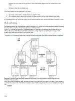
Figure 3-1
Four Input Mux Sym-
bol and Function.

Let’s look at two examples that illustrate this point more clearly. Both
examples are models of a 4 to 1 multiplexer device. The symbol and truth
table for this device are shown in Figure 3-1. One of the four input signals
is propagated to the output depending on the values of inputs A and B.
The first model for the multiplexer is an incorrect model, and the second
is a corrected version of the model.
Incorrect Mux Example
The incorrect model of the multiplexer has a flaw in it that causes the
model to produce incorrect results. This is shown by the following model:
LIBRARY IEEE;
USE IEEE.std_logic_1164.ALL;
ENTITY mux IS
PORT (i0, i1, i2, i3, a, b : IN std_logic;
Chapter Three
44
q : OUT std_logic);
END mux;
ARCHITECTURE wrong of mux IS
SIGNAL muxval : INTEGER;
BEGIN
PROCESS ( i0, i1, i2, i3, a, b )
BEGIN
muxval <= 0;
IF (a = ‘1’) THEN
muxval <= muxval + 1;
END IF;
IF (b = ‘1’) THEN
muxval <= muxval + 2;
END IF;
CASE muxval IS

WHEN 0 =>
q <= I0 AFTER 10 ns;
WHEN 1 =>
q <= I1 AFTER 10 ns;
WHEN 2 =>
q <= I2 AFTER 10 ns;
WHEN 3 =>
q <= I3 AFTER 10 ns;
WHEN OTHERS =>
NULL;
END CASE;
END PROCESS;
END wrong;
Whenever one of the input signals in the process sensitivity list changes
value, the sequential statements in the process are executed. The process
statement in the first example contains four sequential statements. The first
statement initializes the local signal muxval to a known value (0).The sub-
sequent statements add values to the local signal depending on the value
of the a and b input signals. Finally, the case statement chooses an input
to propagate to the output based on the value of signal muxval. This model
has a significant flaw, however. The first statement:
muxval <= 0;
causes the value 0 to be scheduled as an event for signal muxval. In fact,
the value 0 is scheduled in an event for the next simulation delta because
no delay was specified. When the second statement:
IF (a = ‘1’) THEN
muxval <= muxval + 1;
END IF;
45
Sequential Processing

is executed, the value of signal muxval is whatever was last propagated
to it. The new value scheduled from the first statement has not propa-
gated yet. In fact, when multiple assignments to a signal occur within the
same process statement, the last assigned value is the value propagated.
The signal muxval has a garbage value when entering the process. Its
value is not changed until the process has completed execution of all
sequential statements contained in the process. In fact, if signal b is a ‘1’
value, then whatever garbage value the signal had when entering the
process will have the value 2 added to it.
A better way to implement this example is shown in the next example.
The only difference between the next model and the previous one is the
declaration of muxval and the assignments to muxval. In the previous
model, muxval was a signal, and signal assignment statements were used
to assign values to it. In the next example, muxval is a variable, and
variable assignments are used to assign to it.
Correct Mux Example
In this example, the incorrect model is rewritten to reflect a solution to
the problems with the last model:
LIBRARY IEEE;
USE IEEE.std_logic_1164ALL;
ENTITY mux IS
PORT (i0, i1, i2, i3, a, b : IN std_logic;
PORT (q : OUT std_logic);
END mux;
ARCHITECTURE better OF mux IS
BEGIN
PROCESS ( i0, i1, i2, i3, a, b )
VARIABLE muxval : INTEGER;
BEGIN
muxval := 0;

IF (a = ‘1’) THEN
muxval := muxval + 1;
END IF;
IF (b = ‘1’) THEN
muxval := muxval + 2;
END IF;
CASE muxval IS
WHEN 0 =>
q <= I0 AFTER 10 ns;
WHEN 1 =>
Chapter Three
46
q <= I1 AFTER 10 ns;
WHEN 2 =>
q <= I2 AFTER 10 ns;
WHEN 3 =>
q <= I3 AFTER 10 ns;
WHEN OTHERS =>
NULL;
END CASE;
END PROCESS;
END better;
This simple coding difference makes a tremendous operational difference.
When the first statement:
muxval := 0;
is executed, the value 0 is placed in variable muxval immediately. The
value is not scheduled because
muxval, in this example, is a variable, not
a signal. Variables represent local storage as opposed to signals, which
represent circuit interconnect. The local storage is updated immediately,

and the new value can be used later in the model for further computations.
Because
muxval is initialized to 0 immediately, the next two statements
in the process use 0 as the initial value and add appropriate numbers,
depending on the values of signals
a and b. These assignments are also
immediate, and therefore when the
CASE statement executes, variable
muxval contains the correct value. From this value, the correct input signal
can be propagated to the output.
Sequential Statements
Sequential statements exist inside the boundaries of a process statement
as well as in subprograms. In this chapter, we are most concerned with
sequential statements inside process statements. In Chapter 5, we discuss
subprograms and the statements contained within them.
The sequential statements that we discuss are:
■
IF
■ CASE
■ LOOP
■ EXIT
■ ASSERT
■ WAIT
47
Sequential Processing
IF Statements
In Appendix A of the VHDL Language Reference Manual, all VHDL con-
structs are described using a variant of the Bachus-Naur format (BNF)
that is used to describe typical programming languages. If you are not
familiar with BNF, Appendix C gives a cursory description. Becoming

familiar with the BNF will help you better understand how to construct
complex VHDL statements.
The BNF description of the IF statement looks like this:
if_statement ::=
IF condition THEN
sequence_of_statements
{ELSIF condition THEN
sequence_of_statements}
[ELSE
sequence_of_statements]
END IF;
From the BNF description, we can conclude that the IF statement
starts with the keyword IF and ends with the keywords END IF spelled
out as two separate words. There are also two optional clauses: the ELSIF
clause and the ELSE clause. The ELSIF clause is repeatable
—
more than
one ELSIF clause is allowed; but the ELSE clause is optional, and only
one is allowed. The condition construct in all cases is a boolean expres-
sion. This is an expression that evaluates to either true or false. When-
ever a condition evaluates to a true value, the sequence of statements
following is executed. If no condition is true, then the sequence of state-
ments for the ELSE clause is executed, if one exists. Let’s analyze a few
examples to get a better understanding of how the BNF relates to the
VHDL code.
The first example shows how to write a simple
IF statement:
IF (x < 10) THEN
a := b;
END IF;

The IF statement starts with the keyword IF. Next is the condition
(
x < 10), followed by the keyword THEN. The condition is true when the
value of x is less than 10; otherwise it is false. When the condition is true,
the statements between the THEN and END IF are executed. In this exam-
ple, the assignment statement (a := b) is executed whenever x is less than
10. What happens if x is greater than or equal to 10? In this example, there
Chapter Three
48
is no ELSE clause, so no statements are executed in the IF statement. In-
stead, control is transferred to the statement after the END IF.
Let’s look at another example where the ELSE clause is useful:
IF (day = sunday) THEN
weekend := TRUE;
ELSIF (day = saturday) THEN
weekend := TRUE;
ELSE
weekday := TRUE;
END IF;
In this example, there are two variables
—
weekend and weekday
—
that
are set depending on the value of a signal called day. Variable weekend is
set to TRUE whenever day is equal to saturday or sunday. Otherwise, vari-
able weekday is set to TRUE. The execution of the IF statement starts by
checking to see if variable day is equal to sunday. If this is true, then the
next statement is executed and control is transferred to the statement
following END IF. Otherwise, control is transferred to the ELSIF statement

part, and day is checked for saturday. If variable day is equal to saturday,
then the next statement is executed and control is again transferred to the
statement following the END IF statement. Finally, if day is not equal to
sunday or saturday, then the ELSE statement part is executed.
The IF statement can have multiple ELSIF statement parts, but only
one ELSE statement part. More than one sequential statement can exist
between each statement part.
CASE Statements
The CASE statement is used whenever a single expression value can be
used to select between a number of actions. Following is the BNF for the
CASE statement:
case_statement ::=
CASE expression IS
case_statement_alternative
{case_statement_alternative}
END CASE;
case_statement_alternative ::=
WHEN choices =>
49
Sequential Processing
sequence_of_statements
sequence_of_statements ::=
{sequential_statement}
choices ::=
choice{| choice}
choice ::=
SIMPLE_expression|
discrete_range|
ELEMENT_simple_name|
OTHERS

A CASE statement consists of the keyword CASE followed by an expression
and the keyword IS. The expression either returns a value that matches one
of the CHOICES in a WHEN statement part, or matches an OTHERS clause. If the
expression matches the CHOICE part of a WHEN choices => clause, the
sequence_of_statements following is executed. After these statements are
executed, control is transferred to the statement following the END CASE
clause.
Either the CHOICES clause must enumerate every possible value of
the type returned by the expression, or the last choice must contain an
OTHERS clause.
Let’s look at some examples to reinforce what the BNF states:
CASE instruction IS
WHEN load_accum =>
accum <= data;
WHEN store_accum =>
data_out <= accum;
WHEN load|store =>
process_IO(addr);
WHEN OTHERS =>
process_error(instruction);
END CASE;
The CASE statement executes the proper statement depending on the
value of input instruction. If the value of instruction is one of the choices
listed in the WHEN clauses, then the statement following the WHEN clause
is executed. Otherwise, the statement following the OTHERS clause is ex-
ecuted. In this example, when the value of instruction is load_accum, the
first assignment statement is executed. If the value of instruction is load
or store, the process_IO procedure is called.
If the value of instruction is outside the range of the choices given, then
the OTHERS clause matches the expression and the statement following the

Chapter Three
50
OTHERS clause is executed. It is an error if an OTHERS clause does not ex-
ist, and the choices given do not cover every possible value of the expression
type.
In the next example, a more complex type is returned by the expression.
(Types are discussed in Chapter 4, “Data Types.”) The
CASE statement
uses this type to select among the choices of the statement:
TYPE vectype IS ARRAY(0 TO 1) OF BIT;
VARIABLE bit_vec : vectype;
.
.
CASE bit_vec IS
WHEN “00” =>
RETURN 0;
WHEN “01” =>
RETURN 1;
WHEN “10” =>
RETURN 2;
WHEN “11” =>
RETURN 3;
END CASE;
This example shows one way to convert an array of bits into an integer.
When both bits of variable bit_vec contain ‘0’ values, the first choice
“00” matches and the value 0 is returned. When both bits are ‘1’ values,
the value 3, or “11”, is returned. This CASE statement does not need an
OTHERS clause because all possible values of variable bit_vec are enu-
merated by the choices.
LOOP Statements

The LOOP statement is used whenever an operation needs to be repeated.
LOOP statements are used when powerful iteration capability is needed to
implement a model. Following is the BNF for the
LOOP statement:
loop_statement ::=
[LOOP_label : ] [iteration_scheme] LOOP
sequence_of_statements
END LOOP[LOOP_label];
iteration_scheme ::=
WHILE condition | FOR LOOP_parameter_specification
51
Sequential Processing
LOOP_parameter_specification ::=
identifier IN discrete_range
The LOOP statement has an optional label, which can be used to
identify the LOOP statement. The LOOP statement has an optional
iteration_scheme that determines which kind of LOOP statement is being
used. The iteration_scheme includes two types of LOOP statements: a
WHILE condition LOOP statement and a “FOR identifier IN
discrete_range
” statement. The FOR loop loops as many times as specified
in the discrete_range, unless the loop is exited. The WHILE condition
LOOP
statement loops as long as the condition expression is TRUE.
Let’s look at a couple of examples to see how these statements work:
WHILE (day = weekday) LOOP
day := get_next_day(day);
END LOOP;
This example uses the WHILE condition form of the LOOP statement.
The condition is checked each time before the loop is executed. If the condi-

tion is TRUE,the LOOP statements are executed. Control is then transferred
back to the beginning of the loop. The condition is checked again. If TRUE,
the loop is executed again; if not, statement execution continues on the
statement following the END LOOP clause.
The other version of the LOOP statement is the FOR loop:
FOR i IN 1 to 10 LOOP
i_squared(i) := i * i;
END LOOP;
This loop executes 10 times whenever execution begins. Its function is
to calculate the squares from 1 to 10 and insert them into the i_squared
signal array. The index variable i starts at the leftmost value of the range
and is incremented until the rightmost value of the range.
In some languages, the loop index (in this example,
i) can be assigned
a value inside the loop to change its value. VHDL does not allow any
assignment to the loop index. This also precludes the loop index existing
as the return value of a function, or as an out or inout parameter of a
procedure.
Another interesting point about FOR LOOP statements is that the index
value i is locally declared by the FOR statement. The variable i does not
need to be declared explicitly in the process, function, or procedure. By
virtue of the FOR LOOP statement, the loop index is declared locally. If
Chapter Three
52
another variable of the same name exists in the process, function, or
procedure, then these two variables are treated as separate variables
and are accessed by context. Let’s look at an example to illustrate this
point:
PROCESS(i)
BEGIN

x <= i + 1; x is a signal
FOR i IN 1 to a/2 LOOP
q(i) := a; q is a variable
END LOOP;
END PROCESS;
Whenever the value of the signal i in the process sensitivity list
changes value, the process will be invoked. The first statement schedules
the value i + 1 on the signal x. Next, the FOR loop is executed. The index
value i is not the same object as the signal i that was used to calculate
the new value for signal x. These are separate objects that are each
accessed by context. Inside the FOR loop, when a reference is made to i,
the local index is retrieved. But outside the FOR loop, when a reference is
made to i, the value of the signal i in the sensitivity list of the process
is retrieved.
The values used to specify the range in the FOR loop need not be specific
integer values, as has been shown in the examples. The range can
be any discrete range. A discrete_range can be expressed as a
subtype_indication or a range statement. Let’s look at a few more exam-
ples of how FOR loops can be constructed with ranges:
PROCESS(clk)
TYPE day_of_week IS (sun, mon, tue, wed, thur, fri,
sat);
BEGIN
FOR i IN day_of_week LOOP
IF i = sat THEN
son <= mow_lawn;
ELSIF i = sun THEN
church <= family;
ELSE
dad <= go_to_work;

END IF;
END LOOP;
END PROCESS;
53
Sequential Processing
In this example, the range is specified by the type. By specifying the
type as the range, the compiler determines that the leftmost value is sun,
and the rightmost value is sat. The range then is determined as from
sun to sat.
If an ascending range is desired, use the to clause. The downto clause
can be used to create a descending range. Here is an example:
PROCESS(x, y)
BEGIN
FOR i IN x downto y LOOP
q(i) := w(i);
END LOOP;
END PROCESS;
When different values for x and y are passed in, different ranges of the
array w are copied to the same place in array q.
NEXT Statement
There are cases when it is necessary to stop executing the statements in
the loop for this iteration and go to the next iteration. VHDL includes a
construct that accomplishes this. The NEXT statement allows the designer
to stop processing this iteration and skip to the successor. When the NEXT
statement is executed, processing of the model stops at the current point
and is transferred to the beginning of the LOOP statement. Execution begins
with the first statement in the loop, but the loop variable is incremented
to the next iteration value. If the iteration limit has been reached, pro-
cessing stops. If not, execution continues.
Following is an example showing this behavior:

PROCESS(A, B)
CONSTANT max_limit : INTEGER := 255;
BEGIN
FOR i IN 0 TO max_limit LOOP
IF (done(i) = TRUE) THEN
NEXT;
ELSE
done(i) := TRUE;
END IF;
q(i) <= a(i) AND b(i);
END LOOP;
END PROCESS;
Chapter Three
54
The process statement contains one LOOP statement. This LOOP state-
ment logically “and”s the bits of arrays a and b and puts the results in
array q. This behavior continues whenever the flag in array done is not
true. If the done flag is already set for this value of index i, then the NEXT
statement is executed. Execution continues with the first statement of the
loop, and index i has the value i + 1. If the value of the done array is
not true, then the NEXT statement is not executed, and execution continues
with the statement contained in the ELSE clause for the IF statement.
The NEXT statement allows the designer the ability to stop execution of
this iteration and go on to the next iteration. There are other cases when
the need exists to stop execution of a loop completely. This capability is
provided with the EXIT statement.
EXIT Statement
During the execution of a LOOP statement, it may be necessary to jump
out of the loop. This can occur because a significant error has occurred
during the execution of the model or all of the processing has finished

early. The VHDL EXIT statement allows the designer to exit or jump out
of a LOOP statement currently in execution. The EXIT statement causes
execution to halt at the location of the EXIT statement. Execution con-
tinues at the statement following the LOOP statement.
Here is an example illustrating this point:
PROCESS(a)
variable int_a : integer;
BEGIN
int_a := a;
FOR i IN 0 TO max_limit LOOP
IF (int_a <= 0) THEN less than or
EXIT; equal to
ELSE
int_a := int_a -1;
q(i) <= 3.1416 / REAL(int_a * i); signal
END IF; assign
END LOOP;
y <= q;
END PROCESS;
55
Sequential Processing
Inside this process statement, the value of int_a is always assumed to
be a positive value greater than 0. If the value of int_a is negative or zero,
then an error condition results and the calculation should not be com-
pleted. If the value of int_a is less than or equal to 0, then the IF state-
ment is true and the EXIT statement is executed. The loop is immediately
terminated, and the next statement executed is the assignment statement
to y after the LOOP statement.
If this were a complete example, the designer would also want to alert
the user of the model that a significant error had occurred. A method to

accomplish this function would be with an ASSERT statement, which is dis-
cussed later in this chapter.
The EXIT statement has three basic types of operations. The first involves
an EXIT statement without a loop label, or a WHEN condition. If these
conditions are true, then the EXIT statement behaves as follows.
The EXIT statement only exits from the most current LOOP statement
encountered. If an EXIT statement is inside a LOOP statement that is
nested inside another LOOP statement, the EXIT statement only exits the
inner LOOP statement. Execution still remains in the outer LOOP state-
ment. The exit statement only exits from the most recent LOOP statement.
This case is shown in the previous example.
If the EXIT statement has an optional loop label, then the EXIT state-
ment, when encountered, completes the execution of the loop specified by
the loop label. Therefore, the next statement executed is the one following
the END LOOP of the labeled loop. Here is an example:
PROCESS(a)
BEGIN
first_loop: FOR i IN 0 TO 100 LOOP
second_loop:FOR j IN 1 TO 10 LOOP

EXIT second_loop; exits the second loop only

EXIT first_loop; exits the first loop and second
EXIT first_loop; loop
END LOOP;
END LOOP;
END PROCESS;
The first EXIT statement only exits the innermost loop because it com-
pletes execution of the loop labeled second_loop. The last EXIT statement
completes execution of the loop labeled first_loop, which exits from the

first loop and the second loop.
Chapter Three
56
If the EXIT statement has an optional WHEN condition, then the EXIT
statement only exits the loop if the condition specified is true. The next
statement executed depends on whether the EXIT statement has a loop
label specified or not. If a loop label is specified, the next statement executed
is contained in the LOOP statement specified by the loop label. If no loop
label is present, the next statement executed is in the next outer loop. Here
is an example of an EXIT statement with a WHEN condition:
EXIT first_loop WHEN (i < 10);
This statement completes the execution of the loop labeled first_loop
when the expression i < 10 is true.
The EXIT statement provides a quick and easy method of exiting a
LOOP statement when all processing is finished or an error or warning
condition occurs.
ASSERT Statement
The ASSERT statement is a very useful statement for reporting textual
strings to the designer. The ASSERT statement checks the value of a
boolean expression for true or false. If the value is true, the statement
does nothing. If the value is false, the ASSERT statement outputs a user-
specified text string to the standard output to the terminal.
The designer can also specify a severity level with which to output the
text string. The four levels are, in increasing level of severity, note, warn-
ing, error, and failure. The severity level gives the designer the ability to
classify messages into proper categories.
The note category is useful for relaying information to the user about
what is currently happening in the model. For instance, if the model had
a giant loop that took a long time to execute, an assertion of severity level
note could be used to notify the designer when the loop was 10 percent

complete, 20 percent complete, 30 percent complete, and so on.
Assertions of category warning can be used to alert the designer of con-
ditions that, although not catastrophic, can cause erroneous behavior
later. For instance, if a model expected a signal to be at a known value while
some process was executing, but the signal was at a different value, it may
not be an error as in the EXIT statement example, but a warning to the
user that results may not be as expected.