Additional Praise for Fixed Income Securities Tools for Today’s Markets, 2nd Edition phần 2 ppsx
Bạn đang xem bản rút gọn của tài liệu. Xem và tải ngay bản đầy đủ của tài liệu tại đây (617.56 KB, 52 trang )
ward rate curve with views on rates by inspection or by more careful com-
putations will reveal which bonds are cheap and which bonds are rich with
respect to forecasts. It should be noted that the interest rate risk of long-
term bonds differs from that of short-term bonds. This point will be stud-
ied extensively in Part Two.
TREASURY STRIPS, CONTINUED
In the context of the law of one price, Chapter 1 compared the discount fac-
tors implied by C-STRIPS, P-STRIPS, and coupon bonds. With the defini-
tions of this chapter, spot rates can be compared. Figure 2.3 graphs the spot
rates implied from C- and P-STRIPS prices for settlement on February 15,
2001. The graph shows in terms of rate what Figure 1.4 showed in terms of
price. The shorter-maturity C-STRIPS are a bit rich (lower spot rates) while
the longer-maturity C-STRIPS are very slightly cheap (higher spot rates).
Notice that the longer C-STRIPS appear at first to be cheaper in Figure 1.4
than in Figure 2.3. As will become clear in Part Two, small changes in the
spot rates of longer-maturity zeros result in large price differences. Hence
the relatively small rate cheapness of the longer-maturity C-STRIPS in Fig-
ure 2.3 is magnified into large price cheapness in Figure 1.4.
Treasury STRIPS, Continued 37
FIGURE 2.3 Spot Curves Implied by C-STRIPS and P-STRIPS Prices on February
15, 2001
4.500%
5.000%
5.500%
6.000%
6.500%
0 5 10 15 20 25 30
Rate
Spot from C-STRIPS Spot from P-STRIPS
The two very rich P-STRIPS in Figure 2.3, one with 10 and one with
30 years to maturity, derive from the most recently issued bonds in their re-
spective maturity ranges. As mentioned in Chapter 1 and as to be discussed
in Chapter 15, the richness of these bonds and their underlying P-STRIPS
is due to liquidity and financing advantages.
Chapter 4 will show a spot rate curve derived from coupon bonds
(shown earlier as Figure 2.1) that very much resembles the spot rate curve
derived from C-STRIPS. This evidence for the law of one price is deferred
to that chapter, which also discusses curve fitting and smoothness: As can
be seen by comparing Figures 2.1 and 2.3, the curve implied from the raw
C-STRIPS data is much less smooth than the curve constructed using the
techniques of Chapter 4.
APPENDIX 2A
THE RELATION BETWEEN SPOT AND FORWARD
RATES AND THE SLOPE OF THE TERM STRUCTURE
The following proposition formalizes the notion that the term structure of
spot rates slopes upward when forward rates are above spot rates. Simi-
larly, the term structure of spot rates slopes downward when forward rates
are below spot rates.
Proposition 1: If the forward rate from time t to time t+.5 exceeds the
spot rate to time t, then the spot rate to time t+.5 exceeds the spot rate to
time t.
Proof: Since r(t+.5)>rˆ(t),
(2.29)
Multiplying both sides by (1+rˆ(t)/2)
2t
,
(2.30)
Using the relationship between spot and forward rates given in equation
(2.17), the left-hand side of (2.30) can be written in terms of r
ˆ
(t+.5):
1
2
1
5
2
1
2
221
+
+
+
>+
+
ˆ
() ( . )
ˆ
()rt rt rt
tt
1
5
2
1
2
+
+
>+
rt rt(.)
ˆ
()
38 BOND PRICES, SPOT RATES, AND FORWARD RATES
(2.31)
But this implies, as was to be proved, that
(2.32)
Proposition 2: If the forward rate from time t to time t+.5 is less than
the spot rate to time t, then the spot rate to time t+.5 is less than the spot
rate to time t.
Proof: Reverse the inequalities in the proof of proposition 1.
ˆ
(.)
ˆ
()rt rt+>5
1
5
2
1
2
21 21
+
+
>+
++
ˆ
(.)
ˆ
()rt rt
tt
APPENDIX 2A The Relation between Spot and Forward Rates 39
41
CHAPTER
3
Yield-to-Maturity
C
hapters 1 and 2 showed that the time value of money can be de-
scribed by discount factors, spot rates, or forward rates. Further-
more, these chapters showed that each cash flow of a fixed income
security must be discounted at the factor or rate appropriate for the term
of that cash flow.
In practice, investors and traders find it useful to refer to a bond’s
yield-to-maturity, or yield, the single rate that when used to discount a
bond’s cash flows produces the bond’s market price. While indeed useful as
a summary measure of bond pricing, yield-to-maturity can be misleading
as well. Contrary to the beliefs of some market participants, yield is not a
good measure of relative value or of realized return to maturity. In particu-
lar, if two securities with the same maturity have different yields, it is not
necessarily true that the higher-yielding security represents better value.
Furthermore, a bond purchased at a particular yield and held to maturity
will not necessarily earn that initial yield.
Perhaps the most appealing interpretation of yield-to-maturity is not
recognized as widely as it should be. If a bond’s yield-to-maturity remains
unchanged over a short time period, that bond’s realized total rate of re-
turn equals its yield.
This chapter aims to define and interpret yield-to-maturity while high-
lighting its weaknesses. The presentation will show when yields are conve-
nient and safe to use and when their use is misleading.
DEFINITION AND INTERPRETATION
Yield-to-maturity is the single rate such that discounting a security’s cash
flows at that rate produces the security’s market price. For example, Table
1.1 reported the 6
1
/
4
s of February 15, 2003, at a price of 102-18
1
/
8
on Feb-
ruary 15, 2001. The yield-to-maturity of the 6
1
/
4
s, y, is defined such that
(3.1)
Solving for y by trial and error or some numerical method shows that the
yield-to-maturity of this bond is about 4.8875%.
1
Note that given yield in-
stead of price, it is easy to solve for price. As it is so easy to move from
price to yield and back, yield-to-maturity is often used as an alternate way
to quote price. In the example of the 6
1
/
4
s, a trader could just as easily bid
to buy the bonds at a yield of 4.8875% as at a price of 102-18
1
/
8
.
While calculators and computers make price and yield calculations
quite painless, there is a simple and instructive formula with which to re-
late price and yield. The definition of yield-to-maturity implies that the
price of a T-year security making semiannual payments of c/2 and a final
principal payment of F is
2
(3.2)
Note that there are 2T terms being added together through the summation
sign since a T-year bond makes 2T semiannual coupon payments. This
sum equals the present value of all the coupon payments, while the final
term equals the present value of the principal payment. Using the case of
the 6
1
/
4
s of February 15, 2003, as an example of equation (3.2), T=2,
c=6.25, y=4.8875%, F=100, and P=102.5665.
Using the fact that
3
(3.3)
z
zz
z
t
ta
b
ab
=
+
∑
=
−
−
1
1
PT
c
y
F
y
t
t
T
T
()=
+
()
+
+
()
=
∑
2
12 12
1
2
2
3 125
12
3 125
12
3 125
12
103 125
12
102 18 125 32
234
. .
.
+
+
+
()
+
+
()
+
+
()
=+
y
yyy
42 YIELD-TO-MATURITY
1
Many calculators, spreadsheets, and other computer programs are available to
compute yield-to-maturity given bond price and vice versa.
2
A more general formula, valid when the next coupon is due in less than six
months, is given in Chapter 5.
3
The proof of this fact is as follows. Let . Then, and
S–zS=z
a
–z
b+1
. Finally, dividing both sides of this equation by 1–z gives equation (3.3).
Sz
t
ta
b
=
=
∑
zS z
t
ta
b
=
=+
+
∑
1
1
with z=1/(1+
y
/
2
), a=1, and b=2T, equation (3.2) becomes
(3.4)
Several conclusions about the price-yield relationship can be drawn
from equation (3.4). First, when c=100y and F=100, P=100. In words,
when the coupon rate equals the yield-to-maturity, bond price equals
face value, or par. Intuitively, if it is appropriate to discount all of a
bond’s cash flows at the rate y, then a bond paying a coupon rate of c is
paying the market rate of interest. Investors will not demand to receive
more than their initial investment at maturity nor will they accept less
than their initial investment at maturity. Hence, the bond will sell for its
face value.
Second, when c>100y and F=100, P>100. If the coupon rate exceeds
the yield, then the bond sells at a premium to par, that is, for more than
face value. Intuitively, if it is appropriate to discount all cash flows at the
yield, then, in exchange for an above-market coupon, investors will de-
mand less than their initial investment at maturity. Equivalently, investors
will pay more than face value for the bond.
Third, when c<100y, P<100. If the coupon rate is less than the yield,
then the bond sells at a discount to par, that is, for less than face value.
Since the coupon rate is below market, investors will demand more than
their initial investment at maturity. Equivalently, investors will pay less
than face value for the bond.
Figure 3.1 illustrates these first three implications of equation (3.4).
Assuming that all yields are 5.50%, each curve gives the price of a bond
with a particular coupon as a function of years remaining to maturity. The
bond with a coupon rate of 5.50% has a price of 100 at all terms. With 30
years to maturity, the 7.50% and 6.50% coupon bonds sell at substantial
premiums to par, about 129 and 115, respectively. As these bonds mature,
however, the value of above-market coupons falls: receiving a coupon 1%
or 2% above market for 20 years is not as valuable as receiving those
above-market coupons for 30 years. Hence, the prices of these premium
bonds fall over time until they are worth par at maturity. This effect of
time on bond prices is known as the pull to par.
Conversely, the 4.50% and 3.50% coupon bonds sell at substantial
discounts to par, at about 85 and 71, respectively. As these bonds mature,
PT
c
yy
F
y
TT
()=−
+
+
+
1
1
12 12
22
Definition and Interpretation 43
the disadvantage of below-market coupons falls. Hence, the prices of these
bonds rise to par as they mature.
It is important to emphasize that to illustrate simply the pull to par
Figure 3.1 assumes that the bonds yield 5.50% at all times. The actual
price paths of these bonds over time will differ dramatically from those in
the figure depending on the realization of yields.
The fourth implication of equation (3.4) is the annuity formula. An
annuity with semiannual payments is a security that makes a payment c/2
every six months for T years but never makes a final “principal” payment.
In terms of equation (3.4), F=0, so that the price of an annuity, A(T) is
(3.5)
For example, the value of a payment of
6.50
/
2
every six months for 10 years
at a yield of 5.50% is about 46.06.
The fifth implication of equation (3.4) is that as T gets very large,
P=c/y. In words, the price of a perpetuity, a bond that pays coupons for-
ever, equals the coupon divided by the yield. For example, at a yield of
5.50%, a 6.50 coupon in perpetuity will sell for
6.50
/
5.50%
or approximately
AT
c
yy
T
()=−
+
1
1
12
2
44 YIELD-TO-MATURITY
FIGURE 3.1 Prices of Bonds Yielding 5.5% with Various Coupons and Years to
Maturity
60
70
80
90
100
110
120
130
140
Price
30
Coupon = 7.50%
25 20 15 10
5
0
Years to Maturity
Coupon = 6.50%
Coupon = 5.50%
Coupon = 4.50%
Coupon = 3.50%
118.18. While perpetuities are not common, the equation P=c/y provides a
fast, order-of-magnitude approximation for any coupon bond with a long
maturity. For example, at a yield of 5.50% the price of a 6.50% 30-year
bond is about 115 while the price of a 6.50 coupon in perpetuity is about
118. Note, by the way, that an annuity paying its coupon forever is also a
perpetuity. For this reason the perpetuity formula may also be derived
from (3.5) with T very large.
The sixth and final implication of equation (3.4) is the following. If a
bond’s yield-to-maturity over a six-month period remains unchanged, then
the annual total return of the bond over that period equals its yield-to-ma-
turity. This statement can be proved as follows. Let P
0
and P
1/2
be the price
of a T-year bond today and the price
4
just before the next coupon pay-
ment, respectively, assuming that the yield remains unchanged over the six-
month period. By the definition of yield to maturity,
(3.6)
and
(3.7)
Note that after six months have passed, the first coupon payment is not
discounted at all since it will be paid in the next instant, the second coupon
payment is discounted over one six-month period, and so forth, until the
principal plus last coupon payment are discounted over 2T–1 six-month
periods. Inspection of (3.6) and (3.7) reveals that
(3.8)
Rearranging terms,
(3.9)
y
P
P
=−
21
12
0
PyP
12 0
12=+
()
P
cc
y
c
y
T
12
21
2
2
12
12
12
=+
+
++
+
+
()
−
L
P
c
y
c
y
c
y
T
0
22
2
12
2
12
12
12
=
+
+
+
()
++
+
+
()
L
Definition and Interpretation 45
4
In this context, price is the full price. The distinction between flat and full price
will be presented in Chapter 4.
The term in parentheses is the return on the bond over the six-month pe-
riod, and twice that return is the bond’s annual return. Therefore, if yield
remains unchanged over a six-month period, the yield equals the annual re-
turn, as was to be shown.
YIELD-TO-MATURITY AND SPOT RATES
Previous chapters showed that each of a bond’s cash flows must be dis-
counted at a rate corresponding to the timing of that particular cash flow.
Taking the 6
1
/
4
s of February 15, 2003, as an example, the present value of
the bond’s cash flows can be written as a function of its yield-to-maturity,
as in equation (3.1), or as a function of spot rates. Mathematically,
(3.10)
Equations (3.10) clearly demonstrate that yield-to-maturity is a summary
of all the spot rates that enter into the bond pricing equation. Recall from
Table 2.1 that the first four spot rates have values of 5.008%, 4.929%,
4.864%, and 4.886%. Thus, the bond’s yield of 4.8875% is a blend of
these four rates. Furthermore, this blend is closest to the two-year spot rate
of 4.886% because most of this bond’s value comes from its principal pay-
ment to be made in two years.
Equations (3.10) can be used to be more precise about certain relation-
ships between the spot rate curve and the yield of coupon bonds.
First, consider the case of a flat term structure of spot rates; that is, all
of the spot rates are equal. Inspection of equations (3.10) reveals that the
yield must equal that one spot rate level as well.
Second, assume that the term structure of spot rates is upward-sloping;
that is,
(3.11)
In that case, any blend of these four rates will be below rˆ
2
. Hence, the yield
of the two-year bond will be below the two-year spot rate.
ˆˆ ˆˆ
rr rr
2151 5
>>>
102 18 125 32
3 125
12
3 125
12
3 125
12
103 125
12
3 125
12
3 125
12
3 125
12
103 125
12
234
5
1
2
15
3
2
4
+=
+
+
+
()
+
+
()
+
+
()
=
+
+
+
()
+
+
()
+
+
()
.
. .
.
ˆ
.
ˆ
.
ˆ
.
ˆ
.
.
y
yyy
r
rr r
46 YIELD-TO-MATURITY
Third, assume that the term structure of spot rates is downward-slop-
ing. In that case, any blend of the four spot rates will be above rˆ
2
. Hence,
the yield of the two-year bond will be above the two-year spot rate. To
summarize,
Spot rates downward-sloping: Two-year bond yield above two-year
spot rate
Spot rates flat: Two-year bond yield equal to two-year
spot rate
Spot rates upward-sloping: Two-year bond yield below two-year
spot rate
To understand more fully the relationships among the yield of a secu-
rity, its cash flow structure, and spot rates, consider three types of securi-
ties: zero coupon bonds, coupon bonds selling at par (par coupon bonds),
and par nonprepayable mortgages. Mortgages will be discussed in Chapter
21. For now, suffice it to say that the cash flows of a traditional, nonpre-
payable mortgage are level; that is, the cash flow on each date is the same.
Put another way, a traditional, nonprepayable mortgage is just an annuity.
Figure 3.2 graphs the yields of the three security types with varying
Yield-to-Maturity and Spot Rates 47
FIGURE 3.2 Yields of Fairly Priced Zero Coupon Bonds, Par Coupon Bonds, and
Par Nonprepayable Mortgages
4.75%
5.00%
5.25%
5.50%
5.75%
6.00%
0 5 10 15 20 25 30
Term
Yield
Zero Coupon Bonds
Par Coupon Bonds
Par Nonprepayable Mortgages
terms to maturity on February 15, 2001. Before interpreting the graph, the
text will describe how each curve is generated.
The yield of a zero coupon bond of a particular maturity equals the
spot rate of that maturity. Therefore, the curve labeled “Zero Coupon
Bonds” is simply the spot rate curve to be derived in Chapter 4.
This chapter shows that, for a bond selling at its face value, the yield
equals the coupon rate. Therefore, to generate the curve labeled “Par
Coupon Bonds,” the coupon rate is such that the present value of the re-
sulting bond’s cash flows equals its face value. Mathematically, given dis-
count factors and a term to maturity of T years, this coupon rate c satisfies
(3.12)
Solving for c,
(3.13)
Given the discount factors to be derived in Chapter 4, equation (3.13) can
be solved for each value of T to obtain the par bond yield curve.
Finally, the “Par Nonprepayable Mortgages” curve is created as fol-
lows. For comparability with the other two curves, assume that mortgage
payments are made every six months instead of every month. Let X be the
semiannual mortgage payment. Then, with a face value of 100, the present
value of mortgage payments for T years equals par only if
(3.14)
Or, equivalently, only if
(3.15)
Furthermore, the yield of a par nonprepayable T-year mortgage is defined
such that
Xdt
t
T
=
()
=
∑
100 2
1
2
Xdt
t
T
2 100
1
2
()
=
=
∑
c
dT
dt
t
T
=
−
()
[]
()
=
∑
21
2
1
2
100
2
2 100 100
1
2
c
dt dT
t
T
()
+
()
=
=
∑
48 YIELD-TO-MATURITY
(3.16)
Given a set of discount factors, equations (3.15) and (3.16) may be solved
for y
T
using a spreadsheet function or a financial calculator. The “Par Non-
prepayable Mortgages” curve of Figure 3.2 graphs the results.
The text now turns to a discussion of Figure 3.2. At a term of .5 years,
all of the securities under consideration have only one cash flow, which, of
course, must be discounted at the .5-year spot rate. Hence, the yields of all
the securities at .5 years are equal. At longer terms to maturity, the behav-
ior of the various curves becomes more complex.
Consistent with the discussion following equations (3.10), the down-
ward-sloping term structure at the short end produces par yields that ex-
ceed zero yields, but the effect is negligible. Since almost all of the value of
short-term bonds comes from the principal payment, the yields of these
bonds will mostly reflect the spot rate used to discount those final pay-
ments. Hence, short-term bond yields will approximately equal zero
coupon yields.
As term increases, however, the number of coupon payments increases
and discounting reduces the relative importance of the final principal pay-
ment. In other words, as term increases, intermediate spot rates have a
larger impact on coupon bond yields. Hence, the shape of the term struc-
ture can have more of an impact on the difference between zero and par
yields. Indeed, as can be seen in Figure 3.2, the upward-sloping term struc-
ture of spot rates at intermediate terms eventually leads to zero yields ex-
ceeding par yields. Note, however, that the term structure of spot rates
becomes downward-sloping after about 21 years. This shape can be related
to the narrowing of the difference between zero and par yields. Further-
more, extrapolating this downward-sloping structure past the 30 years
recorded on the graph, the zero yield curve will cut through and find itself
below the par yield curve.
The qualitative behavior of mortgage yields relative to zero yields is
the same as that of par yields, but more pronounced. Since the cash flows
of a mortgage are level, mortgage yields are more balanced averages of
spot rates than are par yields. Put another way, mortgage yields will be
more influenced than par bonds by intermediate spot rates. Conse-
quently, if the term structure is downward-sloping everywhere, mortgage
100
1
12
1
2
=
+
()
=
∑
X
y
T
t
t
T
Yield-to-Maturity and Spot Rates 49
yields will be higher than par bond yields. And if the term structure is up-
ward-sloping everywhere, mortgage yields will be lower than par bond
yields. Figure 3.2 shows both these effects. At short terms, the term struc-
ture is downward-sloping and mortgage yields are above par bond yields.
Mortgage yields then fall below par yields as the term structure slopes
upward. As the term structure again becomes downward-sloping, how-
ever, mortgage yields are poised to rise above par yields to the right of the
displayed graph.
YIELD-TO-MATURITY AND RELATIVE VALUE:
THE COUPON EFFECT
All securities depicted in Figure 3.2 are fairly priced. In other words, their
present values are properly computed using a single discount function or
term structure of spot or forward rates. Nevertheless, as explained in the
previous section, zero coupon bonds, par coupon bonds, and mortgages of
the same maturity have different yields to maturity. Therefore, it is incor-
rect to say, for example, that a 15-year zero is a better investment than a
15-year par bond or a 15-year mortgage because the zero has the highest
yield. The impact of coupon level on the yield-to-maturity of coupon
bonds with the same maturity is called the coupon effect. More generally,
yields across fairly priced securities of the same maturity vary with the cash
flow structure of the securities.
The size of the coupon effect on February 15, 2001, can be seen in Fig-
ure 3.2. The difference between the zero and par rates is about 1.3 basis
points
5
at a term of 5 years, 6.1 at 10 years, and 14.1 at 20 years. After
that the difference falls to 10.5 basis points at 25 years and to 2.8 at 30
years. Unfortunately, these quantities cannot be easily extrapolated to
other yield curves. As the discussions in this chapter reveal, the size of the
coupon effect depends very much on the shape of the term structure of in-
terest rates.
50 YIELD-TO-MATURITY
5
A basis point is 1% of .01, or .0001. The difference between a rate of 5.00% and
5.01%, for example, is one basis point.
YIELD-TO-MATURITY AND REALIZED RETURN
Yield-to-maturity is sometimes described as a measure of a bond’s return if
held to maturity. The argument is made as follows. Repeating equation
(3.1), the yield-to-maturity of the 6
1
/
4
s of February 15, 2003, is defined
such that
(3.17)
Multiplying both sides by (1+y/2)
4
gives
(3.18)
The interpretation of the left-hand side of equation (3.18) is as follows. On
August 15, 2001, the bond makes its next coupon payment of 3.125. Semi-
annually reinvesting that payment at rate y through the bond’s maturity of
February 15, 2003, will produce 3.125(1+y/2)
3
. Similarly, reinvesting the
coupon payment paid on February 15, 2002, through the maturity date at
the same rate will produce 3.125(1+y/2)
2
. Continuing with this reasoning,
the left-hand side of equation (3.18) equals the sum one would have on Feb-
ruary 15, 2003, assuming a semiannually compounded coupon reinvest-
ment rate of y. Equation (3.18) says that this sum equals 102.5664(1+y/2)
4
,
the purchase price of the bond invested at a semiannually compounded rate
of y for two years. Hence it is claimed that yield-to-maturity is a measure of
the realized return to maturity.
Unfortunately, there is a serious flaw in this argument. There is ab-
solutely no reason to assume that coupons will be reinvested at the initial
yield-to-maturity of the bond. The reinvestment rate of the coupon paid
on August 15, 2001, will be the 1.5-year rate that prevails six months
from the purchase date. The reinvestment rate of the following coupon
will be the one-year rate that prevails one year from the purchase date,
and so forth. The realized return from holding the bond and reinvesting
coupons depends critically on these unknown future rates. If, for example,
all of the reinvestment rates turn out to be higher than the original yield,
3 125 1 3 125 1 3 125 1 103 125 102 5664 1
2
3
2
2
22
4
+
()
++
()
++
()
+= +
()
yyy y
3 125
12
3 125
12
3 125
12
103 125
12
102 18 125 32
234
. .
.
+
+
+
()
+
+
()
+
+
()
=+
y
yyy
Yield-to-Maturity and Realized Return 51
then the realized yield-to-maturity will be higher than the original yield-
to-maturity. If, at the other extreme, all of the reinvestment rates turn out
to be lower than the original yield, then the realized yield will be lower
than the original yield. In any case, it is extremely unlikely that the real-
ized yield of a coupon bond held to maturity will equal its original yield-
to-maturity. The uncertainty of the realized yield relative to the original
yield because coupons are invested at uncertain future rates is often called
reinvestment risk.
52 YIELD-TO-MATURITY
53
CHAPTER
4
Generalizations and Curve Fitting
W
hile introducing discount factors, bond pricing, spot rates, forward
rates, and yield, the first three chapters simplified matters by assuming
that cash flows appear in even six-month intervals. This chapter general-
izes the discussion of these chapters to accommodate the reality of cash
flows paid at any time. These generalizations include accrued interest built
into a bond’s total transaction price, compounding conventions other than
semiannual, and curve fitting techniques to estimate discount factors for
any time horizon. The chapter ends with a trading case study that shows
how curve fitting may lead to profitable trade ideas.
ACCRUED INTEREST
To ensure that cash flows occur every six months from a settlement date of
February 15, 2001, the bonds included in the examples of Chapters 1
through 3 all matured on either August 15 or on February 15 of a given
year. Consider now the 5
1
/
2
s of January 31, 2003. Since this bond matures
on January 31, its semiannual coupon payments all fall on July 31 or Janu-
ary 31. Therefore, as of February 15, 2001, the latest coupon payment of
the 5
1
/
2
s had been on January 31, 2001, and the next coupon payment was
to be paid on July 31, 2001.
Say that investor B buys $10,000 face value of the 5
1
/
2
s from in-
vestor S for settlement on February 15, 2001. It can be argued that in-
vestor B is not entitled to the full semiannual coupon payment of
$10,000×
5.50%
/
2
or $275 on July 31, 2001, because, as of that time, in-
vestor B will have held the bond for only about five and a half months.
More precisely, since there are 166 days between February 15, 2001,
and July 31, 2001, while there are 181 days between January 31, 2001,
and July 31, 2001, investor B should receive only (
166
/
181
)×$275 or
$252.21 of the coupon payment. Investor S, who held the bond from the
latest coupon date of January 31, 2001, to February 15, 2001, should
collect the rest of the $275 coupon or $22.79. To allow investors B and
S to go their separate ways after settlement, market convention dictates
that investor B pay $22.79 of accrued interest to investor S on the settle-
ment date of February 15, 2001. Furthermore, having paid this $22.79
of accrued interest, investor B may keep the entire $275 coupon pay-
ment of July 31, 2001. This market convention achieves the desired split
of that coupon payment: $22.79 for investor S on February 15, 2001,
and $275–$22.79 or $252.21 for investor B on July 31, 2001. The fol-
lowing diagram illustrates the working of the accrued interest conven-
tion from the point of view of the buyer.
Say that the quoted or flat price of the 5
1
/
2
s of January 31, 2003 on
February 15, 2001, is 101-4
5
/
8
. Since the accrued interest is $22.79 per
$10,000 face or .2279%, the full price of the bond is defined to be
101+
4.625
/
32
+.2279 or 101.3724. Therefore, on $10,000 face amount, the
invoice price—that is, the money paid by the buyer and received by the
seller—is $10,137.24.
The bond pricing equations of the previous chapters have to be gener-
alized to take account of accrued interest. When the accrued interest of a
bond is zero—that is, when the settlement date is a coupon payment
date—the flat and full prices of the bond are equal. Therefore, the previous
chapters could, without ambiguity, make the statement that the price of a
bond equals the present value of its cash flows. When accrued interest is
not zero the statement must be generalized to say that the amount paid or
received for a bond (i.e., its full price) equals the present value of its cash
Last Coupon Purchase Next Coupon
1/ 31 / 01 2 / 15/ 01 7 / 31/ 01
Pay interest
for this period.
Receive interest for the full coupon period.
−−− −−− −−−−−−−−− −−−→|| |
54 GENERALIZATIONS AND CURVE FITTING
flows. Letting P be the bond’s flat price, AI its accrued interest, and PV the
present value function,
(4.1)
Equation (4.1) reveals an important principle about accrued inter-
est. The particular market convention used in calculating accrued inter-
est does not really matter. Say, for example, that everyone believes that
the accrued interest convention in place is too generous to the seller
because instead of being made to wait for a share of the interest until the
next coupon date the seller receives that share at settlement. In that case,
equation (4.1) shows that the flat price adjusts downward to mitigate
this seller’s advantage. Put another way, the only quantity that matters is
the invoice price (i.e., the money that changes hands), and it is this
quantity that the market sets equal to the present value of the future
cash flows.
With an accrued interest convention, if yield does not change then the
quoted price of a bond does not fall as a result of a coupon payment. To
see this, let P
b
and P
a
be the quoted prices of a bond right before and right
after a coupon payment of c/2, respectively. Right before a coupon date the
accrued interest equals the full coupon payment and the present value of
the next coupon equals that same full coupon payment. Therefore, invok-
ing equation (4.1),
(4.2)
Simplifying,
(4.3)
Right after the next coupon payment, accrued interest equals zero. There-
fore, invoking equation (4.1) again,
(4.4)
PPV
a
+=
()
0 cash flows after the next coupon
PPV
b
=
()
cash flows after the next coupon
Pc c PV
b
+=+
()
2 2 cash flows after the next coupon
PAIPV+=(future cash flows)
Accrued Interest 55
Clearly P
a
=P
b
so that the flat price does not fall as a result of the coupon
payment. By contrast, the full price does fall from P
b
+c/2 before the
coupon payment to P
a
=P
b
after the coupon payment.
1
COMPOUNDING CONVENTIONS
Since the previous chapters assumed that cash flows arrive every six months,
the text there could focus on semiannually compounded rates. Allowing for
the possibility that cash flows arrive at any time requires the consideration of
other compounding conventions. After elaborating on this point, this section
argues that the choice of convention does not really matter. Discount factors
are traded, directly through zero coupon bonds or indirectly through coupon
bonds. Therefore, it is really discount factors that summarize market prices
for money on future dates while interest rates simply quote those prices with
the convention deemed most convenient for the application at hand.
When cash flows occur in intervals other than six months, semiannual
compounding is awkward. Say that an investment of one unit of currency
at a semiannual rate of 5% grows to 1+
.05
/
2
after six months. What hap-
pens to an investment for three months at that semiannual rate? The an-
swer cannot be 1+
.05
/
4
, for then a six-month investment would grow to
(1+
.05
/
4
)
2
and not 1+
.05
/
2
. In other words, the answer 1+
.05
/
4
implies quar-
terly compounding. Another answer might be (1+
.05
/
2
)
1/2
. While having the
virtue that a six-month investment does indeed grow to 1+
.05
/
2
, this solu-
tion essentially implies interest on interest within the six-month period.
More precisely, since (1+
.05
/
2
)
1/2
equals (1+
.0497
/
4
), this second solution im-
plies quarterly compounding at a different rate. Therefore, if cash flows do
arrive on a quarterly basis it is more intuitive to discard semiannual com-
pounding and use quarterly compounding instead. More generally, it is
most intuitive to use the compounding convention corresponding to the
smallest cash flow frequency—monthly compounding for payments that
56 GENERALIZATIONS AND CURVE FITTING
1
Note that the behavior of quoted bond prices differs from that of stocks that do
not have an accrued dividend convention. Stock prices fall by approximately the
amount of the dividend on the day ownership of the dividend payment is estab-
lished. The accrued convention does make more sense in bond markets than in
stock markets because dividend payment amounts are generally much less certain
than coupon payments.
may arrive any month, daily compounding for payments that may arrive
any day, and so on. Taking this argument to the extreme and allowing cash
flows to arrive at any time results in continuous compounding. Because of
its usefulness in the last section of this chapter and in the models to be pre-
sented in Part Three, Appendix 4A describes this convention.
Having made the point that semiannual compounding does not suit
every context, it must also be noted that the very notion of compounding
does not suit every context. For coupon bonds, compounding seems nat-
ural because coupons are received every six months and can be reinvested
over the horizon of the original bond investment to earn interest on inter-
est. In the money market, however (i.e., the market to borrow and lend for
usually one year or less), investors commit to a fixed term and interest is
paid at the end of that term. Since there is no interest on interest in the
sense of reinvestment over the life of the original security, the money mar-
ket uses the more suitable choice of simple interest rates.
2
One common simple interest convention in the money market is called
the actual/360 convention.
3
In that convention, lending $1 for d days at a
rate of r will earn the lender an interest payment of
(4.5)
dollars at the end of the d days.
It can now be argued that compounding conventions do not really
matter so long as cash flows are properly computed. Consider a loan from
February 15, 2001, to August 15, 2001, at 5%. Since the number of days
from February 15, 2001, to August 15, 2001, is 181, if the 5% were an ac-
tual/360 rate, the interest payment would be
rd
360
Compounding Conventions 57
2
Contrary to the discussion in the text, personal, short-term time deposits often
quote compound interest rates. This practice is a vestige of Regulation Q that lim-
ited the rate of interest banks could pay on deposits. When unregulated mutual
funds began to offer higher rates, banks competed by increasing compounding fre-
quency. This expedient raised interest payments while not technically violating the
legal rate limits.
3
The accrued interest convention in the Treasury market, described in the previous
section, uses the actual/actual convention: The denominator is set to the actual
number of days between coupon payments.
(4.6)
If the compounding convention were different, however, the interest pay-
ment would be different. Equations (4.7) through (4.9) give interest pay-
ments corresponding to 5% loans from February 15, 2001, to August 15,
2001, under semiannual, monthly, and daily compounding, respectively:
(4.7)
(4.8)
(4.9)
Clearly the market cannot quote a rate of 5% under each of these
compounding conventions at the same time: Everyone would try to borrow
using the convention that generated the lowest interest payment and try to
lend using the convention that generated the highest interest payment.
There can be only one market-clearing interest payment for money from
February 15, 2001, to August 15, 2001.
The most straightforward way to think about this single clearing inter-
est payment is in terms of discount factors. If today is February 15, 2001,
and if August 15, 2001, is considered to be
181
/
365
or .4959 years away, then
in the notation of Chapter 1 the fair market interest payment is
(4.10)
If, for example, d(.4959)=.97561, then the market interest payment is
2.50%. Using equations (4.6) through (4.9) as a model, one can immedi-
ately solve for the simple, as well as the semiannual, monthly, and daily
compounded rates that produce this market interest payment:
1
4959
1
d(. )
−
1
5
365
1 2 5103
181
+
−=
%
.%
1
5
12
1 2 5262
6
+
−=
%
.%
5
2
25
%
.%=
5 181
360
2 5139
%
.%
×
=
58 GENERALIZATIONS AND CURVE FITTING
(4.11)
In summary, compounding conventions must be understood in order
to determine cash flows. But with respect to valuation, compounding con-
ventions do not matter: The market-clearing prices for cash flows on par-
ticular dates are the fundamental quantities.
YIELD AND COMPOUNDING CONVENTIONS
Consider again the 5
1
/
2
s of January 31, 2003, on February 15, 2001. While
the coupon payments from July 31, 2001, to maturity are six months apart,
the coupon payment on July 31, 2001, is only five and a half months or, more
precisely, 166 days away. How does the market calculate yield in this case?
The convention is to discount the next coupon payment by the factor
(4.12)
where y is the yield of the bond and 181 is the total number of days in the
current coupon period. Despite the interpretive difficulties mentioned in
the previous section, this convention aims to quote yield as a semiannually
compounded rate even though payments do not occur in six-month inter-
vals. In any case, coupon payments after the first are six months apart and
can be discounted by powers of 1/(1+
y
/
2
). In the example of the 5
1
/
2
s of
January 31, 2003, the price-yield formula becomes
(4.13)
P
yyyyy
yy
Full
=
+
()
+
+
()
+
()
+
+
()
+
()
+
+
()
+
()
275
12
275
12 12
275
12 12
102 75
12 12
166 181 166 181 166 181 2
166 181 3
.
.
1
12
166 181
+
()
y
/
181
360
2 50 4 9724
2
250 5
1
12
1 2 50 4 9487
1
365
1 2 50 4 9798
6
181
r
r
r
r
r
r
r
r
s
s
sa
sa
m
m
d
d
=⇒=
=⇒=
+
−= ⇒ =
+
−= ⇒ =
.% . %
.% %
.% . %
.% . %
Yield and Compounding Conventions 59
Or, simplifying slightly,
(4.14)
(With the full price given earlier as 101.3724, y=4.879%.)
More generally, if a bond’s first coupon payment is paid in a fraction
τ
of the next coupon period and if there are N semiannual coupon payments
after that, then the price-yield relationship is
(4.15)
BAD DAYS
The phenomenon of bad days is an example of how confusing yields can be
when cash flows are not exactly six months apart. On August 31, 2001,
the Treasury sold a new two-year note with a coupon of 3
5
/
8
% and a matu-
rity date of August 31, 2003. The price of the note for settlement on Sep-
tember 10, 2001, was 100-7
1
/
4
with accrued interest of .100138 for a full
price of 100.32670. According to convention, the cash flow dates of the
bond are assumed to be February 28, 2002, August 31, 2002, February 28,
2003, and August 31, 2003. In actuality, August 31, 2002, is a Saturday so
that cash flow is made on the next business day, September 3, 2002. Also,
the maturity date August 31, 2003, is a Sunday so that cash flow is made
on the next business day, September 2, 2003. Table 4.1 lists the conven-
tional and true cash flow dates.
Reading from the conventional side of the table, the first coupon is 171
days away out of a 181-day coupon period. As discussed in the previous
section, the first exponent is set to
171
/
181
or .94475. After that, exponents
are increased by one. Hence the conventional yield of the note is defined by
the equation
(4.16)
100 32670
1 8125
12
1 8125
12
1 8125
12
101 8125
12
94475 1 94475 2 94475 3 94475
.
. .
=
+
()
+
+
()
+
+
()
+
+
()
yy y y
P
c
yy
Full
i
i
N
N
=
+
()
+
+
()
+
=
+
∑
2
1
12
1
12
0
ττ
P
yy y y
Full
=
+
()
+
+
()
+
+
()
+
+
()
++ +
275
12
275
12
275
12
102 75
12
166 181 166 181 1 166 181 2 166 181 3
. .
60 GENERALIZATIONS AND CURVE FITTING
Solving, the conventional yield equals 3.505%.
Unfortunately, this calculation overstates yield by assuming that the
cash flows arrive sooner than they actually do. To correct for this effect,
the market uses a true yield. Reading from the true side of Table 4.1, the
first cash flow date is unchanged and so is the first exponent. The cash flow
date on September 3, 2002, however, is 187 days from the previous
coupon payment. Defining the number of semiannual periods between
these dates to be
187
/
(365/2)
or 1.02466, the exponent for the second cash
flow date is .94475+1.02466 or 1.96941. Proceeding in this way to calcu-
late the rest of the exponents, the true yield is defined to satisfy the follow-
ing equation:
(4.17)
Solving, the true yield is 3.488%, or 1.7 basis points below the conven-
tional yield.
Professional investors do care about this difference. The lesson for this
section, however, is that forcing semiannual compounding onto dates that
are not six months apart can cause confusion. This confusion, the coupon
effect, and the other interpretive difficulties of yield might suggest avoiding
yield when valuing one bond relative to another.
INTRODUCTION TO CURVE FITTING
Sensible and smooth discount functions and rate curves are useful in a vari-
ety of fixed income contexts.
100 32670
1 8125
12
1 8125
12
1 8125
12
101 8125
12
94475 1 96941 2 94475 3 96393
.
. .
=
+
()
+
+
()
+
+
()
+
+
()
yy y y
Introduction to Curve Fitting 61
TABLE 4.1 Dates for Conventional and True Yield Calculations
Conventional Days to Next Conventional True Days to Next True
Dates Cash Flow Date Exponents Dates Cash Flow Date Exponents
8/31/01 181 8/31/01 181
9/10/01 171 9/10/01 171
2/28/02 184 0.94475 2/28/02 187 0.94475
8/31/02 181 1.94475 9/3/02 178 1.96941
2/28/03 184 2.94475 2/28/03 186 2.94475
8/31/03 3.94475 9/2/03 3.96393