Additional Praise for Fixed Income Securities Tools for Today’s Markets, 2nd Edition phần 3 docx
Bạn đang xem bản rút gọn của tài liệu. Xem và tải ngay bản đầy đủ của tài liệu tại đây (593.19 KB, 52 trang )
89
CHAPTER
5
One-Factor Measures
of Price Sensitivity
T
he interest rate risk of a security may be measured by how much its
price changes as interest rates change. Measures of price sensitivity are
used in many ways, four of which will be listed here. First, traders hedging
a position in one bond with another bond or with a portfolio of other
bonds must be able to compute how each of the bond prices responds to
changes in rates. Second, investors with a view about future changes in in-
terest rates work to determine which securities will perform best if their
view does, in fact, obtain. Third, investors and risk managers need to
know the volatility of fixed income portfolios. If, for example, a risk man-
ager concludes that the volatility of interest rates is 100 basis points per
year and computes that the value of a portfolio changes by $10,000 dollars
per basis point, then the annual volatility of the portfolio is $1 million.
Fourth, asset-liability managers compare the interest rate risk of their as-
sets with the interest rate risk of their liabilities. Banks, for example, raise
money through deposits and other short-term borrowings to lend to corpo-
rations. Insurance companies incur liabilities in exchange for premiums
that they then invest in a broad range of fixed income securities. And, as a
final example, defined benefit plans invest funds in financial markets to
meet obligations to retirees.
Computing the price change of a security given a change in interest
rates is straightforward. Given an initial and a shifted spot rate curve, for
example, the tools of Part One can be used to calculate the price change of
any security with fixed cash flows. Similarly, given two spot rate curves the
models in Part Three can be used to calculate the price change of any de-
rivative security whose cash flows depend on the level of rates. Therefore,
the challenge of measuring price sensitivity comes not so much from the
computation of price changes given changes in interest rates but in defining
what is meant by changes in interest rates.
One commonly used measure of price sensitivity assumes that all bond
yields shift in parallel; that is, they move up or down by the same number
of basis points. Other assumptions are a parallel shift in spot rates or a
parallel shift in forward rates. Yet another reasonable assumption is that
each spot rate moves in some proportion to its maturity. This last assump-
tion is supported by the observation that short-term rates are more volatile
than long-term rates.
1
In any case, there are very many possible definitions
of changes in interest rates.
An interest rate factor is a random variable that impacts interest rates
in some way. The simplest formulations assume that there is only one fac-
tor driving all interest rates and that the factor is itself an interest rate. For
example, in some applications it might be convenient to assume that the
10-year par rate is that single factor. If parallel shifts are assumed as well,
then the change in every other par rate is assumed to equal the change in
the factor, that is, in the 10-year par rate.
In more complex formulations there are two or more factors driving
changes in interest rates. It might be assumed, for example, that the
change in any spot rate is the linearly interpolated change in the two-year
and 10-year spot rates. In that case, knowing the change in the two-year
spot rate alone, or knowing the change in the 10-year spot rate alone,
would not allow for the determination of changes in other spot rates. But
if, for example, the two-year spot rate were known to increase by three
basis points and the 10-year spot rate by one basis point, then the six-year
rate, just between the two- and 10-year rates, would be assumed to in-
crease by two basis points.
There are yet other complex formulations in which the factors are
not themselves interest rates. These models, however, are deferred to
Part Three.
This chapter describes one-factor measures of price sensitivity in full
generality, in particular, without reference to any definition of a change in
rates. Chapter 6 presents the commonly invoked special case of parallel
90 ONE-FACTOR MEASURES OF PRICE SENSITIVITY
1
In countries with a central bank that targets the overnight interest rate, like the
United States, this observation does not apply to the very short end of the curve.
yield shifts. Chapter 7 discusses multi-factor formulations. Chapter 8 shows
how to model interest rate changes empirically.
The assumptions about interest rate changes and the resulting mea-
sures of price sensitivity appearing in Part Two have the advantage of sim-
plicity but the disadvantage of not being connected to any particular
pricing model. This means, for example, that the hedging rules developed
here are independent of the pricing or valuation rules used to determine the
quality of the investment or trade that necessitated hedging in the first
place. At the cost of some complexity, the assumptions invoked in Part
Three consistently price securities and measure their price sensitivities.
DV01
Denote the price-rate function of a fixed income security by P(y), where y
is an interest rate factor. Despite the usual use of y to denote a yield, this
factor might be a yield, a spot rate, a forward rate, or a factor in one of the
models of Part Three. In any case, since this chapter describes one-factor
measures of price sensitivity, the single number y completely describes the
term structure of interest rates and, holding everything but interest rates
constant, allows for the unique determination of the price of any fixed in-
come security.
As mentioned above, the concepts and derivations in this chapter ap-
ply to any term structure shape and to any one-factor description of term
structure movements. But, to simplify the presentation, the numerical ex-
amples assume that the term structure of interest rates is flat at 5% and
that rates move up and down in parallel. Under these assumptions, all
yields, spot rates, and forward rates are equal to 5%. Therefore, with re-
spect to the numerical examples, the precise definition of y does not matter.
This chapter uses two securities to illustrate price sensitivity. The first
is the U.S. Treasury 5s of February 15, 2011. As of February 15, 2001, Fig-
ure 5.1 graphs the price-rate function of this bond. The shape of the graph
is typical of coupon bonds: Price falls as rate increases, and the curve is
very slightly convex.
2
The other security used as an example in this chapter is a one-year
European call option struck at par on the 5s of February 15, 2011. This
DV01 91
2
The discussion of Figure 4.4 defines a convex curve.
option gives its owner the right to purchase some face amount of the bond
after exactly one year at par. (Options and option pricing will be discussed
further in Part Three and in Chapter 19.) If the call gives the right to pur-
chase $10 million face amount of the bond then the option is said to have
a face amount of $10 million as well. Figure 5.2 graphs the price-rate
function. As in the case of bonds, option price is expressed as a percent of
face value.
In Figure 5.2, if rates rise 100 basis points from 3.50% to 4.50%, the
price of the option falls from 11.61 to 5.26. Expressed differently, the
change in the value of the option is (5.26–11.61)/100 or –.0635 per basis
point. At higher rate levels, option price does not fall as much for the same
increase in rate. Changing rates from 5.50% to 6.50%, for example, low-
ers the option price from 1.56 to .26 or by only .013 per basis point.
More generally, letting ∆P and ∆y denote the changes in price and rate
and noting that the change measured in basis points is 10,000×∆y, define
the following measure of price sensitivity:
(5.1)
DV01 is an acronym for dollar value of an ’01 (i.e., .01%) and gives the
change in the value of a fixed income security for a one-basis point decline
DV01 ≡−
×
∆
∆
P
y10 000,
92 ONE-FACTOR MEASURES OF PRICE SENSITIVITY
FIGURE 5.1 The Price-Rate Function of the 5s of February 15, 2011
70
80
90
100
110
120
130
2.00% 3.00% 4.00% 5.00% 6.00% 7.00% 8.00%
Yield
Price
in rates. The negative sign defines DV01 to be positive if price increases
when rates decline and negative if price decreases when rates decline. This
convention has been adopted so that DV01 is positive most of the time: All
fixed coupon bonds and most other fixed income securities do rise in price
when rates decline.
The quantity
∆P
/
∆y
is simply the slope of the line connecting the two
points used to measure that change.
3
Continuing with the option example,
∆P
/
∆y
for the call at 4% might be graphically illustrated by the slope of a line
connecting the points (3.50%, 11.61) and (4.50%, 5.26) in Figure 5.2. It
follows from equation (5.1) that DV01 at 4% is proportional to that slope.
Since the price sensitivity of the option can change dramatically with
the level of rates, DV01 should be measured using points relatively close to
the rate level in question. Rather than using prices at 3.50% and 4.50% to
measure DV01 at 4%, for example, one might use prices at 3.90% and
4.10% or even prices at 3.99% and 4.01%. In the limit, one would use the
slope of the line tangent to the price-rate curve at the desired rate level. Fig-
ure 5.3 graphs the tangent lines at 4% and 6%. That the line AA in this fig-
DV01 93
FIGURE 5.2 The Price-Rate Function of a One-Year European Call Option Struck
at Par on the 5s of February 15, 2011
–5
0
5
10
15
20
25
3.00% 4.00% 5.00% 6.00% 7.00%
Yield
Price
3
The slope of a line equals the change in the vertical coordinate divided by the
change in the horizontal coordinate. In the price-rate context, the slope of the line
is the change in price divided by the change in rate.
ure is steeper than the line BB indicates that the option is more sensitive to
rates at 4% than it is at 6%.
The slope of a tangent line at a particular rate level is equal to the
derivative of the price-rate function at that rate level. The derivative is
written
dP(y)
/
dy
or simply
dP
/
dy
. (The first notation of the derivative empha-
sizes its dependence on the level of rates, while the second assumes
awareness of this dependence.) For readers not familiar with the calcu-
lus, “d” may be taken as indicating a small change and the derivative
may be thought of as the change in price divided by the change in rate.
More precisely, the derivative is the limit of this ratio as the change in
rate approaches zero.
In some special cases to be discussed later,
dP
/
dy
can be calculated ex-
plicitly. In these cases, DV01 is defined using this derivative and
(5.2)
In other cases DV01 must be estimated by choosing two rate levels, com-
puting prices at each of the rates, and applying equation (5.1).
As mentioned, since DV01 can change dramatically with the level of
DV01 =−
()
1
10 000,
dP y
dy
94 ONE-FACTOR MEASURES OF PRICE SENSITIVITY
FIGURE 5.3 A Graphical Representation of DV01 for the One-Year Call on the 5s
of February 15, 2011
–5
0
5
10
15
20
25
Yield
Price
A
A
B
B
4.00% 6.00%
rates it should be measured over relatively narrow ranges of rate.
4
The first
three columns of Table 5.1 list selected rate levels, option prices, and DV01
estimates from Figure 5.2. Given the values of the option at rates of 4.01%
and 3.99%, for example, DV01 equals
(5.3)
In words, with rates at 4% the price of the option falls by about 6.41 cents
for a one-basis point rise in rate. Notice that the DV01 estimate at 4%
does not make use of the option price at 4%: The most stable numerical es-
timate chooses rates that are equally spaced above and below 4%.
Before closing this section, a note on terminology is in order. Most
market participants use DV01 to mean yield-based DV01, discussed in
Chapter 6. Yield-based DV01 assumes that the yield-to-maturity changes
by one basis point while the general definition of DV01 in this chapter al-
lows for any measure of rates to change by one basis point. To avoid con-
fusion, some market participants have different names for DV01 measures
according to the assumed measure of changes in rates. For example, the
change in price after a parallel shift in forward rates might be called DVDF
or DPDF while the change in price after a parallel shift in spot or zero rates
might be called DVDZ or DPDZ.
A HEDGING EXAMPLE, PART I:
HEDGING A CALL OPTION
Since it is usual to regard a call option as depending on the price of a bond,
rather than the reverse, the call is referred to as the derivative security and
the bond as the underlying security. The rightmost columns of Table 5.1
−
×
=−
−
×−
()
=
∆
∆
P
y10 000
8 0866 8 2148
10 000 4 01 3 99
0641
,
,.%.%
.
A Hedging Example, Part I: Hedging a Call Option 95
4
Were prices available without error, it would be desirable to choose a very small
difference between the two rates and estimate DV01 at a particular rate as accu-
rately as possible. Unfortunately, however, prices are usually not available without
error. The models developed in Part Three, for example, perform so many calcula-
tions that the resulting prices are subject to numerical error. In these situations it is
not a good idea to magnify these price errors by dividing by too small a rate differ-
ence. In short, the greater the pricing accuracy, the smaller the optimal rate differ-
ence for computing DV01.
list the prices and DV01 values of the underlying bond, namely the 5s of
February 15, 2011, at various rates.
If, in the course of business, a market maker sells $100 million face
value of the call option and rates are at 5%, how might the market maker
hedge interest rate exposure by trading in the underlying bond? Since the
market maker has sold the option and stands to lose money if rates fall,
bonds must be purchased as a hedge. The DV01 of the two securities may
be used to figure out exactly how many bonds should be bought against
the short option position.
According to Table 5.1, the DV01 of the option with rates at 5% is
.0369, while the DV01 of the bond is .0779. Letting F be the face amount
of bonds the market maker purchases as a hedge, F should be set such that
the price change of the hedge position as a result of a one-basis point
change in rates equals the price change of the option position as a result of
the same one-basis point change. Mathematically,
(5.4)
(Note that the DV01 values, quoted per 100 face value, must be divided by
100 before being multiplied by the face amount of the option or of the
bond.) Solving for F, the market maker should purchase approximately
$47.37 million face amount of the underlying bonds. To summarize this
hedging strategy, the sale of $100 million face value of options risks
F
F
×= ×
=×
.
,,
.
,,
.
.
0779
100
100 000 000
0369
100
100 000 000
0369
0779
96 ONE-FACTOR MEASURES OF PRICE SENSITIVITY
TABLE 5.1 Selected Option Prices, Underlying Bond Prices, and DV01s at
Various Rate Levels
Rate Option Option Bond Bond
Level Price DV01 Price DV01
3.99% 8.2148 108.2615
4.00% 8.1506 0.0641 108.1757 0.0857
4.01% 8.0866 108.0901
4.99% 3.0871 100.0780
5.00% 3.0501 0.0369 100.0000 0.0779
5.01% 3.0134 99.9221
5.99% 0.7003 92.6322
6.00% 0.6879 0.0124 92.5613 0.0709
6.01% 0.6756 92.4903
(5.5)
for each basis point decline in rates, while the purchase of $47.37 million
bonds gains
(5.6)
per basis point decline in rates.
Generally, if DV01 is expressed in terms of a fixed face amount, hedg-
ing a position of F
A
face amount of security A requires a position of F
B
face
amount of security B where
(5.7)
To avoid careless trading mistakes, it is worth emphasizing the simple
implications of equation (5.7), assuming that, as usually is the case, each
DV01 is positive. First, hedging a long position in security A requires a
short position in security B and hedging a short position in security A re-
quires a long position in security B. In the example, the market maker sells
options and buys bonds. Mathematically, if F
A
>0 then F
B
<0 and vice versa.
Second, the security with the higher DV01 is traded in smaller quantity
than the security with the lower DV01. In the example, the market maker
buys only $47.37 million bonds against the sale of $100 million options.
Mathematically, if DV01
A
>DV01
B
then F
B
>–F
A
, while if DV01
A
<DV01
B
then –F
A
>F
B
.
(There are occasions in which one DV01 is negative.
5
In these cases
equation (5.7) shows that a hedged position consists of simultaneous longs
or shorts in both securities. Also, the security with the higher DV01 in ab-
solute value is traded in smaller quantity.)
Assume that the market maker does sell $100 million options and does
buy $47.37 million bonds when rates are 5%. Using the prices in Table
F
F
B
AA
B
=
−×DV01
DV01
$, ,
.
$,47 370 000
0779
100
36 901×=
$,,
.
$,100 000 000
0369
100
36 900×=
A Hedging Example, Part I: Hedging a Call Option 97
5
For an example in the mortgage context see Chapter 21.
5.1, the cost of establishing this position and, equivalently, the value of the
position after the trades is
(5.8)
Now say that rates fall by one basis point to 4.99%. Using the prices
in Table 5.1 for the new rate level, the value of the position becomes
(5.9)
The hedge has succeeded in that the value of the position has hardly
changed even though rates have changed.
To avoid misconceptions about market making, note that the market
maker in this example makes no money. In reality, the market maker
would purchase the option at its midmarket price minus some spread. Tak-
ing half a tick, for example, the market maker would pay half of
1
/
32
or
.015625 less than the market price of 3.0501 on the $100 million for a to-
tal of $15,625. This spread compensates the market maker for effort ex-
pended in the original trade and for hedging the option over its life. Some
of the work involved in hedging after the initial trade will become clear in
the sections continuing this hedging example.
DURATION
DV01 measures the dollar change in the value of a security for a basis
point change in interest rates. Another measure of interest rate sensitivity,
duration, measures the percentage change in the value of a security for a
unit change in rates.
6
Mathematically, letting D denote duration,
(5.10)
D
P
P
y
≡−
1 ∆
∆
−×+×=$,,
.
$, ,
.
$, ,100 000 000
3 0871
100
47 370 000
100 0780
100
44 319 849
−×+×=$,,
.
$, , $, ,100 000 000
3 0501
100
47 370 000
100
100
44 319 900
98 ONE-FACTOR MEASURES OF PRICE SENSITIVITY
6
A unit change means a change of one. In the rate context, a change of one is a
change of 10,000 basis points.
As in the case of DV01, when an explicit formula for the price-rate
function is available, the derivative of the price-rate function may be used
for the change in price divided by the change in rate:
(5.11)
Otherwise, prices at various rates must be substituted into (5.10) to esti-
mate duration.
Table 5.2 gives the same rate levels, option prices, and bond prices as
Table 5.1 but computes duration instead of DV01. Once again, rates a ba-
sis point above and a basis point below the rate level in question are used
to compute changes. For example, the duration of the underlying bond at a
rate of 4% is given by
(5.12)
One way to interpret the duration number of 7.92 is to multiply both
sides of equation (5.10) by ∆y:
(5.13)
∆
∆
P
P
Dy=−
D =−
−
−
=
(. . )/ .
.% .%
.
108 0901 108 2615 108 1757
401 399
792
D
P
dP
dy
≡−
1
Duration 99
TABLE 5.2 Selected Option Prices, Underlying Bond Prices, and Durations at
Various Rate Levels
Rate Option Option Bond Bond
Level Price Duration Price Duration
3.99% 8.2148 108.2615
4.00% 8.1506 78.60 108.1757 7.92
4.01% 8.0866 108.0901
4.99% 3.0871 100.0780
5.00% 3.0501 120.82 100.0000 7.79
5.01% 3.0134 99.9221
5.99% 0.7003 92.6322
6.00% 0.6879 179.70 92.5613 7.67
6.01% 0.6756 92.4903
In the case of the underlying bond, equation (5.13) says that the percentage
change in price equals minus 7.92 times the change in rate. Therefore, a
one-basis point increase in rate will result in a percentage price change of
–7.92×.0001 or –.0792%. Since the price of the bond at a rate of 4% is
108.1757, this percentage change translates into an absolute change of
–.0792%×108.1757 or –.0857. In words, a one-basis point increase in rate
lowers the bond price by .0857. Noting that the DV01 of the bond at a
rate of 4% is .0857 highlights the point that duration and DV01 express
the same interest rate sensitivity of a security in different ways.
Duration tends to be more convenient than DV01 in the investing con-
text. If an institutional investor has $10 million to invest when rates are
5%, the fact that the duration of the option vastly exceeds that of the bond
alerts the investor to the far greater risk of investing money in options.
With a duration of 7.79, a $10 million investment in the bonds will change
by about .78% for a 10-basis point change in rates. However, with a dura-
tion of 120.82, the same $10 million investment will change by about
12.1% for the same 10-basis point change in rates!
In contrast to the investing context, in a hedging problem the dollar
amounts of the two securities involved are not the same. In the example
of the previous section, for instance, the market maker sells options
worth about $3.05 million and buys bonds worth $47.37 million.
7
The
fact that the DV01 of an option is so much less than the DV01 of a bond
tells the market maker that a hedged position must be long much less
face amount of bonds than it is short face amount of options. In the
hedging context, therefore, the dollar sensitivity to a change in rates
(i.e., DV01) is more convenient a measure than the percentage change in
price (i.e., duration).
Tables 5.1 and 5.2 illustrate the difference in emphasis of DV01 and
duration in another way. Table 5.1 shows that the DV01 of the option de-
clines with rates, while Table 5.2 shows that the duration of the option in-
creases with rates. The DV01 numbers show that for a fixed face amount
of option the dollar sensitivity declines with rates. Since, however, declin-
ing rates also lower the price of the option, percentage price sensitivity, or
duration, actually increases.
100 ONE-FACTOR MEASURES OF PRICE SENSITIVITY
7
To finance this position the market maker will borrow the difference between
these dollar amounts. See Chapter 15 for a discussion about financing positions.
Like the section on DV01, this section closes with a note on terminol-
ogy. As defined in this chapter, duration may be computed for any assumed
change in the term structure of interest rates. This general definition is also
called effective duration. Many market participants, however, use the term
duration to mean Macaulay duration or modified duration, discussed in
Chapter 6. These measures of interest rate sensitivity explicitly assume a
change in yield-to-maturity.
CONVEXITY
As mentioned in the discussion of Figure 5.3 and as seen in Tables 5.1
and 5.2, interest rate sensitivity changes with the level of rates. To illus-
trate this point more clearly, Figure 5.4 graphs the DV01 of the option
and underlying bond as a function of the level of rates. The DV01 of the
bond declines relatively gently as rates rise, while the DV01 of the op-
tion declines sometimes gently and sometimes violently depending on
the level of rates. Convexity measures how interest rate sensitivity
changes with rates.
Convexity 101
FIGURE 5.4 DV01 of the 5s of February 15, 2011, and of the Call Option as a
Function of Rates
0
0.02
0.04
0.06
0.08
0.1
0.12
2.00% 3.00% 4.00% 5.00% 6.00% 7.00% 8.00%
Yield
DV01
Call Option
5s of 2/15/2011
Mathematically, convexity is defined as
(5.14)
where d
2
P/dy
2
is the second derivative of the price-rate function. Just as the
first derivative measures how price changes with rates, the second deriva-
tive measures how the first derivative changes with rates. As with DV01
and duration, if there is an explicit formula for the price-rate function then
(5.14) may be used to compute convexity. Without such a formula, con-
vexity must be estimated numerically.
Table 5.3 shows how to estimate the convexity of the bond and the op-
tion at various rate levels. The convexity of the bond at 5%, for example,
is estimated as follows. Estimate the first derivative between 4.99% and
5% (i.e., at 4.995%) by dividing the change in price by the change in rate:
(5.15)
Table 5.3 displays price to four digits but more precision is used to calcu-
late the derivative estimate of –779.8264. This extra precision is often nec-
essary when calculating second derivatives.
Similarly, estimate the first derivative between 5% and 5.01% (i.e., at
5.005%) by dividing the change in the corresponding prices by the change
100 100 0780
5499
780
−
−
=−
.
%.%
C
P
dP
dy
=
1
2
2
102 ONE-FACTOR MEASURES OF PRICE SENSITIVITY
TABLE 5.3 Convexity Calculations for the Bond and Option at Various Rates
Rate Bond First Option First
Level Price Derivative Convexity Price Derivative Convexity
3.99% 108.2615 8.2148
4.00% 108.1757 –857.4290 75.4725 8.1506 –641.8096 2,800.9970
4.01% 108.0901 –856.6126 8.0866 –639.5266
4.99% 100.0780 3.0871
5.00% 100.0000 –779.8264 73.6287 3.0501 –369.9550 9,503.3302
5.01% 99.9221 –779.0901 3.0134 –367.0564
5.99% 92.6322 0.7003
6.00% 92.5613 –709.8187 71.7854 0.6879 –124.4984 25,627.6335
6.01% 92.4903 –709.1542 0.6756 –122.7355
in rate to get –779.0901. Then estimate the second derivative at 5% by di-
viding the change in the first derivative by the change in rate:
(5.16)
Finally, to estimate convexity, divide the estimate of the second derivative
by the bond price:
(5.17)
Both the bond and the option exhibit positive convexity. Mathemati-
cally positive convexity simply means that the second derivative is positive
and, therefore, that C >0. Graphically this means that the price-rate curve
is convex. Figures 5.1 and 5.2 do show that the price-rate curves of both
bond and option are, indeed, convex. Finally, the property of positive con-
vexity may also be thought of as the property that DV01 falls as rates in-
crease (see Figure 5.4).
Fixed income securities need not be positively convex at all rate levels.
Some important examples of negative convexity are callable bonds (see the
last section of this chapter and Chapter 19) and mortgage-backed securi-
ties (see Chapter 21).
Understanding the convexity properties of securities is useful for both
hedging and investing. This is the topic of the next few sections.
A HEDGING EXAMPLE, PART II:
A SHORT CONVEXITY POSITION
In the first section of this hedging example the market maker buys $47.37
million of the 5s of February 15, 2011, against a short of $100 million op-
tions. Figure 5.5 shows the profit and loss, or P&L, of a long position of
$47.37 million bonds and of a long position of $100 million options as
rates change. Since the market maker is actually short the options, the
P&L of the position at any rate level is the P&L of the long bond position
minus the P&L of the long option position.
By construction, the DV01 of the long bond and option positions are
the same at a rate level of 5%. In other words, for small rate changes, the
C
P
P
y
===
1 7 363
100
73 63
2
2
∆
∆
,
.
∆
∆
2
2
779 0901 779 8264
5 005 4 995
7 363
P
y
=
−+
−
=
.%.%
,
A Hedging Example, Part II: A Short Convexity Position 103
change in the value of one position equals the change in the value of the
other. Graphically, the P&L curves are tangent at 5%.
The previous section of this example shows that the hedge performs
well in that the market maker neither makes nor loses money after a one-
basis point change in rates. At first glance it may appear from Figure 5.5
that the hedge works well even after moves of 50 basis points. The values
on the vertical axis, however, are measured in millions. After a move of
only 25 basis points, the hedge is off by about $80,000. This is a very large
number in light of the approximately $15,625 the market maker collected
in spread. Worse yet, since the P&L of the long option position is always
above that of the long bond position, the market maker loses this $80,000
whether rates rise or fall by 25 basis points.
The hedged position loses whether rates rise or fall because the option
is more convex than the bond. In market jargon, the hedged position is
short convexity. For small rate changes away from 5% the values of the
bond and option positions change by the same amount. Due to its greater
convexity, however, the sensitivity of the option changes by more than the
sensitivity of the bond. When rates increase, the DV01 of both the bond
and the option fall but the DV01 of the option falls by more. Hence, after
further rate increases, the option falls in value less than the bond, and the
P&L of the option position stays above that of the bond position. Simi-
104 ONE-FACTOR MEASURES OF PRICE SENSITIVITY
FIGURE 5.5 P&L of Long Positions in the 5s of February 15, 2011, and in the
Call Option
–15.00
–10.00
–5.00
0.00
5.00
10.00
15.00
20.00
25.00
2.00% 3.00% 4.00% 5.00% 6.00% 7.00% 8.00%
Yield
P&L ($millions)
Call Option
5s of 2/15/2011
larly, when rates decline below 5%, the DV01 of both the bond and option
rise but the DV01 of the option rises by more. Hence, after further rate de-
clines the option rises in value more than the bond, and the P&L of the op-
tion position again stays above that of the bond position.
This discussion reveals that DV01 hedging is local, that is, valid in a
particular neighborhood of rates. As rates move, the quality of the hedge
deteriorates. As a result, the market maker will need to rehedge the posi-
tion. If rates rise above 5% so that the DV01 of the option position falls by
more than the DV01 of the bond position, the market maker will have to
sell bonds to reequate DV01 at the higher level of rates. If, on the other
hand, rates fall below 5% so that the DV01 of the option position rises by
more than the DV01 of the bond position, the market maker will have to
buy bonds to reequate DV01 at the lower level of rates.
An erroneous conclusion might be drawn at this point. Figure 5.5
shows that the value of the option position exceeds the value of the bond
position at any rate level. Nevertheless, it is not correct to conclude that
the option position is a superior holding to the bond position. In brief, if
market prices are correct, the price of the option is high enough relative to
the price of the bond to reflect its convexity advantages. In particular,
holding rates constant, the bond will perform better than the option over
time, a disadvantage of a long option position not captured in Figure 5.5.
In summary, the long option position will outperform the long bond posi-
tion if rates move a lot, while the long bond position will outperform if
rates stay about the same. It is in this sense, by the way, that a long con-
vexity position is long volatility while a short convexity position is short
volatility. In any case, Chapter 10 explains the pricing of convexity in
greater detail.
ESTIMATING PRICE CHANGES AND RETURNS
WITH DV01, DURATION, AND CONVEXITY
Price changes and returns as a result of changes in rates can be estimated
with the measures of price sensitivity used in previous sections. Despite the
abundance of calculating machines that, strictly speaking, makes these ap-
proximations unnecessary, an understanding of these estimation tech-
niques builds intuition about the behavior of fixed income securities and,
with practice, allows for some rapid mental calculations.
A second-order Taylor approximation of the price-rate function with
Estimating Price Changes and Returns with DV01, Duration, and Convexity 105
respect to rate gives the following approximation for the price of a security
after a small change in rate:
(5.18)
Subtracting P from both sides and then dividing both sides by P gives
(5.19)
Then, using the definitions of duration and convexity in equations (5.11)
and (5.14),
(5.20)
In words, equation (5.20) says that the percentage change in the
price of a security (i.e., its return) is approximately equal to minus the
duration multiplied by the change in rate plus half the convexity multi-
plied by the change in rate squared. As an example, take the price, dura-
tion, and convexity of the call option on the 5s of February 15, 2011,
from Tables 5.2 and 5.3. Equation (5.20) then says that for a 25-basis
point increase in rates
(5.21)
At a starting price of 3.0501, the approximation to the new price is 3.0501
minus .27235×3.0501 or .83070, leaving 2.2194. Since the option price
when rates are 5.25% is 2.2185, the approximation of equation (5.20) is
relatively accurate.
In the example applying (5.20), namely equation (5.21), the duration
term of about 30% is much larger than the convexity term of about 3%.
This is generally true. While convexity is usually a larger number than
duration, for relatively small changes in rate the change in rate is so
much larger than the change in rate squared that the duration effect dom-
inates. This fact suggests that it may sometimes be safe to drop the con-
%
.%
∆P =− × +
()
×
=− +
=−
120 82 0025 1 2 9503 3302 0025
30205 02970
27 235
2
∆
∆∆
P
P
Dy Cy≈− +
1
2
2
∆
∆∆
P
PP
dP
dy
y
P
dP
dy
y≈+×
11
2
1
2
2
2
Py y Py
dP
dy
y
dP
dy
y+
()
≈
()
++∆∆∆
1
2
2
2
2
106 ONE-FACTOR MEASURES OF PRICE SENSITIVITY
vexity term completely and to use the first-order approximation for the
change in price:
(5.22)
This approximation follows directly from the definition of duration and,
therefore, basically repeats equation (5.13).
Figure 5.6 graphs the option price, the first-order approximation
of (5.22), and the second-order approximation of (5.20). Both approxi-
mations work well for very small changes in rate. For larger changes
the second-order approximation still works well, but for very large
changes it, too, fails. In any case, the figure makes clear that approxi-
mating price changes with duration ignores the curvature or convexity
of the price-rate function. Adding a convexity term captures a good deal
of this curvature.
In the case of the bond price, both approximations work so well that
displaying a price graph over the same range of rates as Figure 5.6 would
make it difficult to distinguish the three curves. Figure 5.7, therefore,
graphs the bond price and the two approximations for rates greater than
5%. Since the option is much more convex than the bond, it is harder to
∆
∆
P
P
Dy≈−
Estimating Price Changes and Returns with DV01, Duration, and Convexity 107
FIGURE 5.6 First and Second Order Approximations to Call Option Price
—10
—5
0
5
10
15
20
25
30
3.00% 4.00% 5.00% 6.00% 7.00%
Yield
Price
Price
1st Order
Approximation
2nd Order
Approximation
capture its curvature with the one-term approximation (5.22) or even with
the two-term approximation (5.20).
CONVEXITY IN THE INVESTMENT AND
ASSET-LIABILITY MANAGEMENT CONTEXTS
For very convex securities duration may not be a safe measure of return. In
the example of approximating the return on the option after a 25-basis
point increase in rates, duration used alone overstated the loss by about
3%. Similarly, since the duration of very convex securities can change dra-
matically as rate changes, an investor needs to monitor the duration of in-
vestments. Setting up an investment with a particular exposure to interest
rates may, unattended, turn into a portfolio with a very different exposure
to interest rates.
Another implication of equation (5.20), mentioned briefly earlier, is
that an exposure to convexity is an exposure to volatility. Since ∆y
2
is al-
ways positive, positive convexity increases return so long as interest
rates move. The bigger the move in either direction, the greater the gains
from positive convexity. Negative convexity works in the reverse. If C is
negative, then rate moves in either direction reduce returns. This is an-
other way to understand why a short option position DV01-hedged with
108 ONE-FACTOR MEASURES OF PRICE SENSITIVITY
FIGURE 5.7 First and Second Order Approximations to Price of 5s of
February 15, 2011
80
82
84
86
88
90
92
94
96
98
100
5.00% 5.50% 6.00% 6.50% 7.00% 7.50% 8.00%
Yield
Price
Price
2nd Order
Approximation
1st Order
Approximation
bonds loses money whether rates gap up or down (see Figure 5.5). In the
investment context, choosing among securities with the same duration
expresses a view on interest rate volatility. Choosing a very positively
convex security would essentially be choosing to be long volatility, while
choosing a negatively convex security would essentially be choosing to
be short volatility.
Figures 5.6 and 5.7 suggest that asset-liability managers (and hedgers,
where possible) can achieve greater protection against interest rate changes
by hedging duration and convexity instead of duration alone. Consider an
asset-liability manager who sets both the duration and convexity of assets
equal to those of liabilities. For any interest rate change, the change in the
value of assets will more closely resemble the change in the value of liabili-
ties than had duration alone been matched. Furthermore, since matching
convexity sets the change in interest rate sensitivity of the assets equal to
that of the liabilities, after a small change in rates the sensitivity of the as-
sets will still be very close to the sensitivity of the liabilities. In other words,
the asset-liability manager need not rebalance as often as in the case of
matching duration alone.
MEASURING THE PRICE SENSITIVITY
OF PORTFOLIOS
This section shows how measures of portfolio price sensitivity are related
to the measures of its component securities. Computing price sensitivities
can be a time-consuming process, especially when using the term structure
models of Part Three. Since a typical investor or trader focuses on a partic-
ular set of securities at one time and constantly searches for desirable port-
folios from that set, it is often inefficient to compute the sensitivity of every
portfolio from scratch. A better solution is to compute sensitivity measures
for all the individual securities and then to use the rules of this section to
compute portfolio sensitivity measures.
A price or measure of sensitivity for security i is indicated by the sub-
script i, while quantities without subscripts denote portfolio quantities. By
definition, the value of a portfolio equals the sum of the value of the indi-
vidual securities in the portfolio:
(5.23)
PP
i
=
∑
Measuring the Price Sensitivity of Portfolios 109
Recall from the introduction to this chapter that y is a single rate or factor
sufficient to determine the prices of all securities. Therefore, one can com-
pute the derivative of price with respect to this rate or factor for all securi-
ties in the portfolio and, from (5.23),
(5.24)
Dividing both sides of by 10,000,
(5.25)
Finally, using the definition of DV01 in equation (5.2),
(5.26)
In words, the DV01 of a portfolio is the sum of the individual DV01 val-
ues.
The rule for duration is only a bit more complex. Starting from equa-
tion (5.24), divide both sides by –P.
(5.27)
Multiplying each term in the summation by one in the form P
i
/P
i
,
(5.28)
Finally, using the definition of duration from (5.11),
(5.29)
In words, the duration of a portfolio equals a weighted sum of individual
durations where each security’s weight is its value as a percentage of port-
folio value.
D
P
P
D
i
i
=
∑
−=−
∑
11
P
dP
dy
P
PP
dP
dy
i
i
i
−=−
∑
11
P
dP
dy P
dP
dy
i
DV01 DV01=
∑
i
1
10 000
1
10 000,,
dP
dy
dP
dy
i
=
∑
dP
dy
dP
dy
i
=
∑
110 ONE-FACTOR MEASURES OF PRICE SENSITIVITY
The formula for the convexity of a portfolio can be derived along the
same lines as the duration of a portfolio, so the convexity result is given
without proof:
(5.30)
The next section applies these portfolio results to the case of a callable
bond.
A HEDGING EXAMPLE, PART III:
THE NEGATIVE CONVEXITY OF CALLABLE BONDS
A callable bond is a bond that the issuer may repurchase or call at some
fixed set of prices on some fixed set of dates. Chapter 19 will discuss
callable bonds in detail and will demonstrate that the value of a callable
bond to an investor equals the value of the underlying noncallable bond
minus the value of the issuer’s embedded option. Continuing with the ex-
ample of this chapter, assume for pedagogical reasons that there exists a
5% Treasury bond maturing on February 15, 2011, and callable in one
year by the U.S. Treasury at par. Then the underlying noncallable bond is
the 5s of February 15, 2011, and the embedded option is the option intro-
duced in this chapter, namely the right to buy the 5s of February 15, 2011,
at par in one year. Furthermore, the value of this callable bond equals the
difference between the value of the underlying bond and the value of the
option.
Figure 5.8 graphs the price of the callable bond and, for comparison,
the price of the 5s of February 15, 2011. Chapter 19 will discuss why the
callable bond price curve has the shape that it does. For the purposes of
this chapter, however, notice that for all but the highest rates in the graph
the callable bond price curve is concave. This implies that the callable bond
is negatively convex in these rate environments.
Table 5.4 uses the portfolio results of the previous section and the re-
sults of Tables 5.1 through 5.3 to compute the DV01, duration, and con-
vexity of the callable bond at three rate levels. At 5%, for example, the
callable bond price is the difference between the bond price and the option
price: 100–3.0501 or 96.9499. The DV01 of the callable bond price is the
difference between the DV01 values listed in Table 5.1: .0779–.0369 or
C
P
P
C
i
i
=
∑
A Hedging Example, Part III: The Negative Convexity of Callable Bonds 111
.0410. The convexity of the callable bond is the weighted sum of the indi-
vidual convexities listed in Table 5.3:
(5.31)
A market maker wanting to hedge the sale of $100 million callable
bonds with the 5s of February 15, 2011, would have to buy $100 million
times the ratio of the DV01 measures or, in millions of dollars,
100×
.0411
/
.0779
or 52.76. Figure 5.9 graphs the P&L from a long position in
the callable bonds and from a long position in this hedge.
The striking aspect of Figure 5.9 is that the positive convexity of the
bond and the negative convexity of the callable bond combine to make the
103 15 73 63 3 15 9 503 33 223.% . .% , .×− × =−
112 ONE-FACTOR MEASURES OF PRICE SENSITIVITY
TABLE 5.4 Price, DV01, Duration, and Convexity of Callable Bond
Rate Callable Bond Fraction Option Fraction Callable Callable Callable
Level Price Price of Value Price of Value DV01 Duration Convexity
4.00% 100.0251 108.1757 108.15% 8.1506 –8.15% 0.0216 2.162983 –146.618
5.00% 96.9499 100.0000 103.15% 3.0501 –3.15% 0.0411 4.238815 –223.039
6.00% 91.8734 92.5613 100.75% 0.6879 –0.75% 0.0586 6.376924 –119.563
FIGURE 5.8 Price of Callable Bond and of 5s of February 15, 2011
70
80
90
100
110
120
130
2.00% 3.00% 4.00% 5.00% 6.00% 7.00% 8.00%
Yield
Price
5s of 2/15/2011
Callable Bond
DV01 hedge quite unstable away from 5%. Not only do the values of the
two securities increase or decrease away from 5% at different rates, as is
also the case in Figure 5.5, but in Figure 5.9 the values are driven even fur-
ther apart by opposite curvatures. In summary, care must be exercised
when mixing securities of positive and negative convexity because the re-
sulting hedges or comparative return estimates are inherently unstable.
A Hedging Example, Part III: The Negative Convexity of Callable Bonds 113
FIGURE 5.9 P&L from Callable Bond and from 5s of February 15, 2011, Hedge
–$200,000
–$150,000
–$100,000
–$50,000
$0
$50,000
$100,000
$150,000
$200,000
2.00% 3.00% 4.00% 5.00% 6.00% 7.00% 8.00%
Yield
P&L
5s of 2/15/2011 Hedge
Callable Bond