Additional Praise for Fixed Income Securities Tools for Today’s Markets, 2nd Edition phần 8 pot
Bạn đang xem bản rút gọn của tài liệu. Xem và tải ngay bản đầy đủ của tài liệu tại đây (690.23 KB, 52 trang )
of futures contracts, the value of a futures contract after its mark to market
payment must equal zero. Putting these two facts together,
(17.10)
Then, solving for the unknown futures price,
(17.11)
Since the same logic applies to the down state of date 1,
(17.12)
As of date 0, setting the expected discounted mark-to-market payment
equal to zero implies that
(17.13)
Or,
(17.14)
Substituting (17.11) and (17.12) into (17.14),
(17.15)
In words, under the risk-neutral process the futures price equals the
expected price of the underlying security as of the delivery date. More
generally,
(17.16)
FUTURES ON RATES IN A TERM STRUCTURE MODEL
The final settlement price of a Eurodollar futures contract is 100 minus the
90-day rate. Therefore, the final contract prices are not P
2
uu
, P
2
ud
, and P
2
dd
, as
FEPM0
()
=
()
[]
F PPPP
PPP
uu ud ud dd
uu ud dd
03322
352
2222
222
()
=× +× +× +×
=× +× +×
FFF
ud
06 4
11
()
=× +×
6040
1
0
11
0
×−
()
()
+× −
()
()
+
=
FF FF
r
ud
FP P
duddd
12 2
55=× +×
FP P
uuuud
12 2
55=× +×
55
1
0
21 21
1
×−
()
+× −
()
+
=
PF PF
r
uu u ud u
u
Futures on Rates in a Term Structure Model 349
in the previous section, but rather 100–r
2
uu
, 100–r
2
ud
, and 100–r
2
dd
. Follow-
ing the logic of the previous section after this substitution, the futures price
equals the expected value of these outcomes. Denoting the rate on date M
by r(M) and the futures price based on the rates as F
R
(0),
(17.17)
Defining the futures rate on date 0, r
fut
, to be 100 minus the futures
price,
(17.18)
THE FUTURES-FORWARD DIFFERENCE
This section brings together the results of Chapter 16 and of the two previ-
ous sections to be more explicit about the difference between forward and
futures prices and between futures and forward rates.
By the definition of covariance, for two random variables G and H,
(17.19)
Letting G=P(M) and H=1/∏(1+r
m
), equation (17.19) becomes
(17.20)
In words, this covariance equals the expected discounted value minus the
discounted expected value. Substituting (17.7), (17.8), and (17.16) into
equation (17.20) and rearranging terms,
(17.21)
Finally, substitute (17.9) into (17.21) to obtain
(17.22)
F P Cov P M
r
dM
fwd
m
0
1
1
0
()
=−
()
+
()
∏
,(,)
F
P
dM
Cov P M
r
dM
m
0
0
0
1
1
0
()
=
()
()
−
()
+
()
()
∏
,
,,
Cov P M
r
E
PM
r
EPM E
r
mm m
()
+
()
=
()
+
()
−
()
[]
+
()
∏∏ ∏
,
1
11
1
1
Cov G H E G H E G E H,
()
=×
[]
−
[]
×
[]
rFErM
fut
R
=−
()
=
()
[]
100 0
FErM
ErM
R
0 100
100
()
=−
()
[]
=−
()
[]
350 EURODOLLAR AND FED FUNDS FUTURES
Combining (17.22) with the meaning of the covariance term, the difference
between the forward price and the futures price is proportional to the dif-
ference between the expected discounted value and the discounted ex-
pected value.
Since the price of the security on date M is likely to be relatively low if
rates from now to date M are relatively high and the price is likely to be
relatively high if rates from now to date M are relatively low, the covari-
ance term in equation (17.22) is likely to be positive.
5
If this is indeed the
case, it follows that
(17.23)
The intuition behind equations (17.22) and (17.23) was mentioned in
the section about tails. Assume for a moment that the futures and forward
price of a security are the same. Daily changes in the value of the forward
contract generate no cash flows while daily changes in the value of the fu-
tures contract generate mark-to-market payments. While mark-to-market
gains can be reinvested and mark-to-market losses must be financed, on av-
erage these effects do not cancel out. Rather, on average they make futures
contracts less desirable than forward contracts. As bond prices tend to fall
when short-term rates are high, when futures suffer a loss this loss has to
be financed at relatively high rates. But, when futures enjoy a gain, this
gain is reinvested at relatively low rates. On average then, if the futures and
forward prices are the same, a long futures position is not so valuable as a
long forward position. Therefore, the two contracts are priced properly
relative to one another only if the futures price is lower than the forward
price, as stated by (17.23).
The discussion to this point is sufficient for note and bond futures,
treated in detail in Chapter 20. For Eurodollar futures, however, it is more
FP
fwd
0
()
<
The Futures-Forward Difference 351
5
This discussion does not necessary apply to forwards and futures on securities out-
side the fixed income context. Consider, for example, a forward and a future on oil.
In this case it is more difficult to determine the covariance between the discounting
factor and the underlying security. If this covariance happens to be positive, then
equation (17.23) holds for oil. But if the covariance is zero, then forward and fu-
tures prices are the same. Similarly, if the covariance is negative, then futures prices
exceed forward prices.
common to express the difference between futures and forward contracts
in terms of rates rather than prices.
Given forward prices of zero coupon bonds, forward rates are com-
puted as described in Chapter 2. If P
fwd
denotes the forward price of a 90-
day zero, the simple interest forward, r
fwd
is such that
(17.24)
The Eurodollar futures rate is given by (17.18). To compare the futures
and forward rates, note that
(17.25)
where the first equality is (17.16) and the second follows from the defin-
itions of P(M), r(M), and simple interest. Using a special case of Jensen’s
Inequality,
6
(17.26)
Finally, combining (17.18), (17.23), (17.24), (17.25), and (17.26),
(17.27)
This equation shows that the difference between forwards and futures
on rates has two separate effects. The first inequality represents the dif-
ference between the forward price and the futures on a price. This differ-
ence is properly called the futures-forward effect. The second inequality
represents the difference between a futures on a price and a futures on a
rate which, as evident from (17.26), is a convexity effect. The sum, ex-
pressed as the difference between the observed forward rates on deposits
and Eurodollar futures rates, will be referred to as the total
futures-forward effect.
P
r
F
r
fwd
fwd fut
=
+×
>
()
>
+×
1
1 90 360
0
1
1 90 360
E
rM
ErM
1
1 90 360
1
1 90 360
+×
()
>
+×
()
[]
FEPME
rM
0
1
1 90 360
()
=
()
[]
=
+×
()
P
r
fwd
fwd
=
+×
1
1 90 360
352 EURODOLLAR AND FED FUNDS FUTURES
6
See equation (10.6).
It follows immediately from (17.27) that
(17.28)
According to (17.28), the futures rate exceeds the forward rate or, equiva-
lently, the total futures-forward difference is positive. But, since the futures-
forward effect depends on the covariance term in equation (17.22), the
magnitude of this effect depends on the particular term structure model be-
ing used. It is beyond the mathematical level of this book to compute the fu-
tures-forward effect for a given term structure model. However, to illustrate
orders of magnitude, results from a particularly simple model are invoked.
In a normal model with no mean reversion, continuous compounding, and
continuous mark-to-market payments, the difference between the futures
rate and the forward rate of a zero due to the pure futures-forward effect is
(17.29)
where
σ
2
is the annual basis point volatility of the short-term rate and t is
the time to expiration, in years, of the forward or futures contract. In the
same model, the difference due to the convexity effect is
(17.30)
where
β
is the maturity, in years, of the underlying zero. The total differ-
ence between the futures and forward rates is the sum of (17.29) and
(17.30). In the case of Eurodollar futures on 90-day deposits,
β
is approxi-
mately .25 and the convexity effect is approximately
σ
2
t/8. Note that, ex-
cept for very small times to expiration, the difference due to the pure
futures-forward effect is larger than that due to the convexity effect and,
for long times to expiration, the contribution of the convexity effect to the
difference is negligible.
Figure 17.1 graphs the total futures-forward effect for each contract as
of November 30, 2001, in the simple model described assuming that
volatility is 100 basis points a year across the curve. The graph illustrates
that, as evident from equation (17.29), the effect increases with the square
of time to contract expiration.
EDH2 matures on December 20, 2002, about .3 years from the pricing
date. For this contract, the total futures-forward effect in basis points is
practically zero:
σβ
2
2t
σ
22
2t
rr
fut fwd
>
The Futures-Forward Difference 353
(17.31)
The effect is not trivial, though, for later-maturing contracts. EDZ6 ma-
tures on December 20, 2006, about 5.05 years from the pricing date. In
this case the total futures-forward effect in basis points is
(17.32)
And, as can be seen from the graph, for the contracts with the longest ex-
piry the effect approaches 50 basis points.
The terms (17.29) and (17.30) explicitly show that the total futures-
forward effect increases with interest rate volatility. The pure futures-for-
ward effect arises because mark-to-market gains are invested at low rates
while mark-to-market losses are financed at high rates. With no interest
rate volatility there are no mark-to-market cash flows and no investment
or financing of those flows. The convexity effect also disappears without
volatility, as demonstrated in Chapter 10.
10 000
01 5 05
2
01 5 05
8
13 4
222
,
.×
×
+
×
=
10 000
01 3
2
01 3
8
0825
22 2
,
.×
×
+
×
=
354 EURODOLLAR AND FED FUNDS FUTURES
FIGURE 17.1 Futures-Forward Effect in a Normal Model with No Mean
Reversion and an Annual Volatility of 100 Basis Points
EDZ1
EDH2
EDM2
EDU2
EDZ2
EDH3
EDM3
EDU3
EDZ3
EDH4
EDM4
EDU4
EDZ4
EDH5
EDM5
EDU5
EDZ5
EDH6
EDM6
EDU6
EDZ6
EDH7
EDM7
EDU7
EDZ7
EDH8
EDM8
EDU8
EDZ8
EDH9
EDM9
EDU9
EDZ9
EDH0
EDM0
EDU0
EDZ0
EDH1
EDM1
EDU1
0
10
20
30
40
50
Contract
Futures-Forward Effect (bps)
TED SPREADS
As discussed in Part Three, making judgments about the value of a security
relative to other securities requires that traders and investors select some
securities that they consider to be fairly priced. Eurodollar futures are of-
ten, although certainly not always, thought of as fairly priced for two
somewhat related reasons. First, they are quite liquid relative to many
other fixed income securities. Second, they are immune to many individual
security effects that complicate the determination of fair value for other se-
curities. Consider, for example, a two-year bond issued by the Federal Na-
tional Mortgage Association (FNMA), a government-sponsored enterprise
(GSE). The price of this bond relative to FNMA bonds of similar maturity
is determined by its supply outstanding, its special repo rate, and the distri-
bution of its ownership across investor classes. Hence, interest rates im-
plied by this FNMA bond might be different from rates implied by similar
FNMA bonds for reasons unrelated to the time value of money. With 90-
day Eurodollar futures, by contrast, there is only one contract reflecting the
time value of money over a particular three-month period. Also, there is no
limit to the supply of any Eurodollar futures contract: whenever a new
buyer and seller appear a new contract is created. In short, the prices of
Eurodollar contracts are much less subject to the idiosyncratic forces im-
pacting the prices of particular bonds.
TED spreads
7
use rates implied by Eurodollar futures to assess the
value of a security relative to Eurodollar futures rates or to assess the value
of one security relative to another. The idea is to find the spread such that
discounting cash flows at Eurodollar futures rates minus that spread pro-
duces the security’s market price. Put another way, it is the negative of the
option-adjusted-spread (OAS) of a bond when Eurodollar futures rates are
used for discounting.
As an example, consider the FNMA 4s of August 15, 2003, priced as
of November 30, 2001, to settle on the next business day, December 3,
2001. The next cash flow of the bond is on February 15, 2002. Referring
to Table 17.1, EDZ1 indicates that the three-month futures rate starting
TED Spreads 355
7
TED spreads were originally used to compare T-bill futures, which are no longer
actively traded, and Eurodollar futures. The name came from the combination of T
for Treasury and ED for Eurodollar.
from December 19, 2001, is 1.9175%. Assume that the rate on the stub—
the period of time from the settlement date to the beginning of the period
spanned by the first Eurodollar contract—is 2.085%. (This stub rate can
be calculated from various short-term LIBOR rates.) Since there are 16
days from December 3, 2001, to December 19, 2001, and 58 days from
December 19, 2001, to February 15, 2002, the discount factor applied to
the first coupon payment using futures rates is
(17.33)
Subtracting a spread s, this factor becomes
(17.34)
The next coupon payment is due on August 15, 2002. Table 17.3 shows
the relevant Eurodollar futures contracts and rates required to discount the
August 15, 2002, coupon. Adding a spread to these rates, this factor is
(17.35)
Proceeding in this way, using the Eurodollar futures rates from Table
17.1, the present value of each payment can be expressed in terms of the
TED spread.
8
The next step is to find the spread such that the sum of these
present values equals the full price of the bond.
1
11 11
2 085 16
360
1 9175 91
360
205 91
360
250 57
360
+
()
+
()
+
()
+
()
−
()
×−
()
×−
()
×−
()
×. % . % .% .%s sss
1
11
02085 16
360
019175 58
360
+
()
+
()
−
()
×−
()
×.% . %ss
1
11
02085 16
360
019175 58
360
+
()
+
()
××.% . %
356 EURODOLLAR AND FED FUNDS FUTURES
TABLE 17.3 Discounting the August 15, 2002,
Coupon Payment
From To Days Symbol Rate(%)
12/3/01 12/19/01 16 STUB 2.0850
12/19/01 03/20/01 91 EDZ1 1.9175
3/20/01 06/19/01 91 EDH2 2.0500
6/19/01 08/15/01 57 EDM2 2.5000
8
Since February 15, 2003, falls on a weekend, the coupon payment due on that
date is deferred to the next business day, in this case February 17, 2003. This actual
payment date is used in the TED spread calculation.
The price of the FNMA 4s of August 15, 2003, on November 30,
2001, was 101.7975. The first coupon payment and the accrued interest
calculation differ from the examples of Chapter 4. First, these agency
bonds were issued with a short first coupon. The issue date, from which
coupon interest begins to accrue, was not August 15, 2001, but August 27,
2001. Put another way, the first coupon payment represents interest not
from August 15, 2001, to February 15, 2002, as is usually the case, but
from August 27, 2001, to February 15, 2002. Consequently, the first
coupon payment will be less than half of the annual 4%. Second, unlike
the U.S. Treasury market, the U.S. agency market uses a 30/360-day count
convention that assumes each month has 30 days. Table 17.4 illustrates
this convention by computing the number of days from August 27, 2001,
to February 15, 2002. Note the assumption that there are only three days
from August 27, 2001, to the end of August, that there are 30 days in Oc-
tober, and so on.
The coupon payment on February 15, 2001, is assumed to cover the
168 days computed in Table 17.4 out of a six-month coupon period of
180 days. At an annual rate of 4%, the semiannual coupon payment
is, therefore,
(17.36)
4
2
168
180
1 8667
%
.%=
TED Spreads 357
TABLE 17.4 Example of the
30/360 Convention: The
Number of Days from August
27, 2001, to February 15, 2002
From To Days
8/27/01 08/30/01 3
9/1/01 09/30/01 30
10/1/01 10/30/01 30
11/1/01 11/30/01 30
12/1/01 12/30/01 30
1/1/02 01/30/02 30
2/1/02 02/15/02 15
Total 168
All subsequent coupon payments are, as usual, 2% of face value.
To determine the accrued interest for settlement on December 3, 2001,
calculate the number of 30/360 days from August 27, 2001, to December
3, 2001. Since this comes to 96 days, the accrued interest is
(17.37)
To summarize, for settlement on December 3, 2001, the price of
101.7975 plus accrued interest of 1.0667 gives an invoice price of
102.8642. The first coupon payment of 1.8667, later coupon payments of
2, and the terminal principal payment are discounted using the discount
factors, described earlier, which depend on the TED spread s. Solving pro-
duces a TED spread of 15.6 basis points.
The interpretation of this TED spread is that the agency is 15.6 basis
points rich to LIBOR as measured by the futures rates. Whether these 15.6
basis points are justified or not requires more analysis. Most importantly, is
the superior credit quality of FNMA relative to that of the banks used to fix
LIBOR worth 15.6 basis points on a bond with approximately two years to
maturity? Chapter 18 will treat this type of question in more detail.
As mentioned earlier, a TED spread may be used not only to measure
the value of a bond relative to futures rates but also to measure the value of
one bond relative to another. The FNMA 4.75s of November 14, 2003, for
example, priced at 103.1276 as of November 30, 2001, had a TED spread
of 20.5 basis points. One might argue that it does not make sense for the
4.75s of November 14, 2003, to trade 20.5 basis points rich to LIBOR
while the 4s of August 15, 2003, maturing only three months earlier, trade
only 15.6 basis points rich.
9
The following section describes how to trade
this difference in TED spreads.
Discounting a bond’s cash flows using futures rates has an obvious
theoretical flaw. According to the results of Part One, discounting should
be done at forward rates, not futures rates. But, as shown in the previous
section, the magnitude of the difference between forward and futures rates
is relatively small for futures expiring shortly. The longest futures rate re-
quired to discount the cash flows of the 4.75s of November 14, 2003, is
4
2
96
180
1 0667
%
.%=
358 EURODOLLAR AND FED FUNDS FUTURES
9
The two bonds finance at equivalent rates in the repo market.
EDU3 expiring on September 15, 2003, that is, about 1.8 years from the
settlement date of December 3, 2001. Using the simple model mentioned
in the previous section with a volatility of 100 basis points in order to
record an order of magnitude, (17.29) and (17.30) combine to produce a
total futures-forward difference for EDU3 of about 1.8 basis points. In
addition, when using TED spreads to compare one bond to a similar
bond, discounting with futures rates instead of forward rates uses rates
too high for both bonds. This means that the relative valuation of the two
bonds is probably not very much affected by the theoretically incorrect
choice of discounting rates.
APPLICATION: Trading TED Spreads
A trader believes that the FNMA 4s of August 15, 2003, are too cheap to LIBOR at a TED
spread of 15.6 basis points, or, equivalently, that the TED spread should be higher. To take
advantage of this perceived mispricing the trader plans to buy $100,000,000 face of the
bonds and to sell Eurodollar futures. How many of each futures contract should be sold?
The procedure is as follows.
1. Decrease a futures rate by one basis point.
2. Keeping the TED spread unchanged, calculate the value of $100,000,000 of the
bond with this perturbed rate and subtract the market price of the position. In
other words, calculate the bucket risk of the position with respect to that futures
rate.
3. Divide the bucket risk by $25, the value of one basis point to a position of one Eu-
rodollar contract.
4. Repeat steps 1 to 3 for all pertinent futures rates.
For example, decreasing EDU2 from 3.055% to 3.045% while keeping the TED spread at
15.6 basis points raises the invoice price of the bond from 102.8642 to 102.866685. On a
position of $100,000,000 this price change is worth
(17.38)
Therefore, to hedge against a change in EDU2 of one basis point, sell
$2,485
/
$25
or about 99
contracts. Repeating this exercise for each contract gives the results in Table 17.5.
Intuitively, since the value of the bonds is about $103,000,000, hedging a forward rate
$,, . % . %$,100 000 000 102 866685 102 8642 2 485×−
(
)
=
APPLICATION: Trading TED Spreads 359
with a $1,000,000 futures contract requires about 103 contracts. Stub risk, of course, an
exposure of only 16 days, requires only 18 contracts: 103×
16
/
91
equals 18. The full 103 con-
tracts of EDZ1 are required, but the tail reduces the required number of contracts with later
expirations. The tail on the EDH3, for example, reduces the hedge by six contracts. The re-
duced amount of EDM3 is mostly because the contract is required to cover only 57 days of
risk and partly because of the tail. (The relevant number of days for the stub and EDM3 cal-
culations appear in Table 17.3.)
Summing the number of contracts in Table 17.5, 681 contracts should be sold against
the bonds. Imagine that all Eurodollar rates increase by one basis point but that the price of
the 4s of August 15, 2003, stays the same. The short position in Eurodollar futures will
make 681×$25 or $17,025, while the bond position will, by assumption, not change in
value. At the same time, by the definition of a TED spread, the TED spread of the bond will
increase from 15.6 to 16.6 basis points. In this sense the trade described profits $17,025
for each TED spread basis point.
The same caveat with respect to valuing bonds using TED spreads must be made with
respect to hedging bonds with Eurodollar futures contracts. If volatility were to increase,
the futures-forward difference would increase. But if forward rates rise relative to futures
rates, a position long bonds and short futures will lose money. This is an unintended expo-
sure of the trade described arising from hedging bond prices or forwards with futures.
Again, however, for relatively short-term securities the effect is usually small.
The other trade suggested by the previous section is to buy the 4s of August 15, 2003,
at a TED of 15.6 basis points and sell the 4.75s of November 14, 2003, at a TED of 20.5 ba-
sis points. This trade is typically designed not to express an opinion about the absolute
360 EURODOLLAR AND FED FUNDS FUTURES
TABLE 17.5 Hedging
$100,000,000 of FNMA 4s of
August 15, 2003, with
Eurodollar Futures
Contract Number
Symbol to Sell
STUB 18
EDZ1 103
EDH2 102
EDM2 101
EDU2 99
EDZ2 99
EDH3 97
EDM3 62
level of TED spreads but, rather, to express the opinion that the TED of the 4.75s of Novem-
ber 15, 2003, is too high relative to that of the 4s of August 15,2003. In trader jargon, this
trade is usually intended to express an opinion about the spread of spreads.
To construct a spread of spreads trade, first calculate the DV01 values of the two
bonds. In this case the values are 1.67 for the 4s of August 15, 2003, and 1.91 for the
4.75s of November 15, 2003, implying a sale of $87,434,600 4.75s against a purchase of
$100,000,000 4s. Next, calculate the Eurodollar futures position required to put on a TED
spread trade for each leg of the position. Third, net out the Eurodollar futures positions.
Table 17.6 shows the results of these steps. Viewing the trade as a combination of two
TED spreads makes it clear that the trade will make money if the TED of the 4s of August
15, 2003, rises and if the TED of the 4.75s of November 15, 2003, falls. But it is the hedg-
ing of the DV01 of the bonds that makes the trade a pure bet on the spread of spreads. The
DV01 hedge forces the sum of the net Eurodollar futures contracts to equal approximately
zero.
10
This means that if bond prices do not change but all futures rates increase or de-
crease by one basis point, so that both TED spreads increase or decrease by one basis
point, then the trade will not make or lose money. In other words, the trade makes or loses
APPLICATION: Trading TED Spreads 361
TABLE 17.6 Spread of Spreads Trade
Buy $100,000,000 FNMA 4s of August 15, 2003
Sell $87,434,600 FNMA 4.75s of November 15, 2003
Futures Futures
Contract to Sell vs. to Buy vs. Net
Symbol 8/03s 11/03s Purchase
STUB 18 16 –2
EDZ1 103 91 –12
EDH2 102 90 –12
EDM2 101 89 –12
EDU2 99 88 –11
EDZ2 99 87 –12
EDH3 97 86 –11
EDM3 62 84 22
EDU3 53 53
10
The net futures position is not exactly zero because DV01 is based on the change of semiannually com-
pounded rates rather than 30/360 rates. If the bond holdings are set so that the net futures position is ex-
actly zero, then the trade will be exactly neutral with respect to parallel shifts in futures rates but not
exactly neutral with respect to equal changes in bond yields.
money only if the TED spreads change relative to one another, as intended. Without the
DV01 hedge, the net position in Eurodollar futures contracts would not be zero and the
trade would make or lose money if bond prices stayed the same while all futures rates
rose or fell by one basis point.
Chapter 18 will present asset swap spreads that measure the value of a bond relative
to the swap curve and asset swap trades that trade bonds against swaps. While asset swap
spreads are a more accurate way to value a bond relative to LIBOR, TED spreads are still
useful for two reasons. First, for bonds maturing within a few years, TED spreads are rela-
tively accurate. Second, for bonds of relatively short maturity, TED spread trades are easier
to execute than asset swap trades because Eurodollar futures of relatively short maturity
are more liquid than swaps of relatively short maturity.
FED FUNDS
In the course of doing business, banks often find that they have cash bal-
ances to invest or cash deficits to finance. The market in which banks trade
funds overnight to manage their cash balances is called the federal funds or
fed funds market. While only banks can borrow or lend in the fed funds
market, the importance of banks in the financial system causes other short-
term interest rates to move with the fed funds rate.
The Board of Governors of the Federal Reserve System (“the Fed”)
sets monetary policy in the United States. An important component of this
policy is the targeting or pegging of the fed funds rate at a level consistent
with price stability and economic well-being. Since banks trade freely in
the fed funds market, the Fed cannot directly set the fed funds rate. But, by
using the tools at its disposal, including buying and selling short-term secu-
rities or repo on short-term securities, the Fed has enormous power to in-
fluence the fed funds rate and to keep it close to the desired target.
The Federal Reserve calculates and publishes the weighted average
rate at which banks borrow and lend money in the fed funds market over
each business day. This rate is called the fed funds effective rate. Figure
17.2 shows the time series of the fed funds target rate against the effec-
tive rate from January 1994 to September 2001. For the most part, the
Fed succeeds in keeping the fed funds rate close to the target rate. The av-
erage difference between the two rates over the sample period is only 2.2
basis points.
While the fed funds rate is usually close to the target rate, Figure
362 EURODOLLAR AND FED FUNDS FUTURES
17.2 shows that the two rates are sometimes very far apart. Sometimes
this happens because temporary, sharp swings in the demand or supply of
funds are not, for one reason or another, counterbalanced by the Fed.
Other times, the Fed decides to abandon its target temporarily in pursuit
of some other policy objective. During times of financial upheaval, for
example, the value of liquidity or cash rises dramatically. Individuals
might rush to withdraw cash from their bank accounts. Banks, other fi-
nancial institutions, and corporations might be reluctant to lend cash,
even if it were secured by collateral. (See the application at the end of
Chapter 15.) As a result, otherwise sound and creditworthy institutions
might become insolvent as a consequence of not being able to raise funds.
At times like these the Fed “injects liquidity into the system” by lending
cash on acceptable collateral. As a result of this action, the fed funds ef-
fective rate might very well drop below the stated target rate. There are
two particularly recent and dramatic examples of this in Figure 17.2.
First, the Fed injected liquidity in anticipation of Y2K problems that
never, in fact, materialized. This resulted in the fed funds rate on Decem-
ber 31, 1999, being about 150 basis points below target. Second, to con-
tain the financial disruption following the events of September 11, 2001,
the Fed injected liquidity and the fed funds rate fell to about 180 basis
points below target.
Fed Funds 363
FIGURE 17.2 The Fed Funds Effective Rate versus the Fed Funds Target Rate
0
1
2
3
4
5
6
7
8
1/3/1994 2/9/1995 3/17/1996 4/23/1997 5/30/1998 7/6/1999 8/11/2000 9/17/2001
Rate (%)
Effective Fed Funds Target Fed Funds
FED FUNDS FUTURES
Like Eurodollar futures, fed funds futures provide another means by which
to hedge exposure to short-term interest rates. Table 17.7 lists the liquid
fed funds contracts as of December 4, 2001. Note that the symbol is a con-
catenation of “FF” for fed funds, a letter indicating the month of the con-
tract, and a digit for the year of the contract.
The fed funds futures contract is designed as a hedge to a $5,000,000
30-day deposit in fed funds. First, the final settlement price of a fed funds
contract in a particular month is set to 100 minus 100 times the average of
the effective fed funds rate over that month. In November 2001, for exam-
ple, the average rate was 2.087% so the contract settled at 97.913. Second,
since changing the rate of a $5,000,000 30-day loan by one basis point
changes the interest payment by
(17.39)
the mark-to-market payment of the contract is set at $41.67 per basis
point.
To see how the fed funds futures contract works as a hedge, consider
the case of a small regional bank that has surplus cash of $5,000,000 over
the month of November 2001. The bank plans to lend this $5,000,000
overnight in the fed funds market over the month but wants to hedge the
risk that a falling fed funds rate will reduce the interest earned in the fed
funds market. Therefore, the bank buys one November fed funds futures
contract at the close of business on October 31, 2001, for 97.79, implying
a rate of 2.21%.
$, ,
.
$.5 000 000
0001 30
360
41 67×
×
=
364 EURODOLLAR AND FED FUNDS FUTURES
TABLE 17.7 Fed Funds Futures as of December
4, 2001
Symbol Expiration Price Rate
FFZ1 12/31/01 98.155 1.845
FFF2 01/31/02 98.235 1.765
FFG2 02/28/02 98.290 1.710
FFH2 03/31/02 98.245 1.755
FFJ2 04/30/02 98.200 1.800
FFK2 05/30/02 98.100 1.900
Recalling that the average fed funds rate in November 2001 was
2.087, over the month the bank earns interest of
11
(17.40)
Also, an average rate of 2.087% implies a final settlement price of 97.913, so
the bank gains 97.913–97.79 or 12.3 basis points on its fed funds contract.
At $41.67 per basis point, the total gain comes to 12.3×$41.67 or $512.54.
Together with the interest payment then, the bank earns $9,208.37. But this is
almost exactly the interest implied by the 2.21% rate of the fed funds futures
contract purchased on October 31, 2001:
(17.41)
Hence, by combining lending in the fed funds market and trading in fed
funds futures, the bank can lock in the lending rate implied by the fed
funds contracts.
Note that the hedge is easy to calculate for any other amount of sur-
plus cash. If the bank has $20,000,000 to invest, for example, the hedge
would be to buy four fed funds contracts: Since each contract has a no-
tional amount of $5,000,000, four contracts are required to hedge an in-
vestment of $20,000,000.
To hedge over a month with 28 or 31 days, the number of contracts has
to be adjusted very slightly. The contract value of $41.67 per basis point is
based on 30 days of interest. To hedge a loan with 28 days of interest re-
quires
28
/
30
times the amount of the investment. So, hedging a $100,000,000
investment over February requires 20×(
28
/
30
) or 19 contracts. Similarly,
$, ,
.%
$, .5 000 000
221 30
360
9 208 33×
×
=
$, ,
.%
$, .5 000 000
2 087 30
360
8 695 83×
×
=
Fed Funds Futures 365
11
This hedging example implicitly assumes that the bank does not earn interest on
interest on its fed funds lending. This is consistent with the assumption of the fed
funds contract that the relevant interest rate is the average of effective fed funds
over the month. To the extent that the bank does earn interest on interest, the fed
funds contract setting is not consistent with the lending context and the hedge
works less precisely. And, while discussing approximations, since fed funds futures
are usually liquid for only the next five months or so, tails are not usually big
enough to warrant attention.
hedging a $100,000,000 investment over December requires 20×(
31
/
30
) or
21 contracts.
This hedging example uses a bank because only banks can participate
in the fed funds market. But, as mentioned earlier, many short-term rates
are highly correlated with the fed funds rate. Therefore, other financial in-
stitutions, corporations, and investors can use fed funds futures to hedge
their individual short-term rate risk. For example, in October 2001 a cor-
poration discovers that it needs to borrow money over the month of De-
cember. To hedge against the risk that rates rise and increase the cost of
borrowing, the company can sell December fed funds futures. While this
hedge will protect the corporation from changes in the general level of in-
terest rates, fed funds futures will not protect against corporate borrowing
rates rising relative to fed funds nor, of course, against that particular cor-
poration’s borrowing rate rising relative to other rates. The difference be-
tween the actual risk (e.g., changes in a corporation’s borrowing rate) and
the risk reduced by the hedge (e.g., changes in the fed funds rate) is an ex-
ample of basis risk.
APPLICATION: Fed Funds Contracts and Predicted Fed Action
Under the chairmanship of Alan Greenspan the Fed has established informal and unofficial
rules under which it changes the fed funds target rate. In particular, the Fed usually changes
the target by some multiple of 25 basis points only after announcing the change at the con-
clusion of a regularly scheduled Federal Open Market Committee (FOMC) meeting. But this
rule is not always followed: On April 18, 2001, the Fed announced a surprise cut in the tar-
get rate from 5% to 4.5%. For the most part, however, the current policy of the Fed is to
take action on FOMC meeting dates.
The prices of fed funds futures imply a particular view about the future actions of the
Fed. Consider the following data as of December 4, 2001.
1. The fed funds target rate is 2%.
2. The average fed funds effective rate from December 1, 2001, to December 4,
2001, was 2.025%.
3. The next FOMC meeting is scheduled for December 11, 2001.
4. The December fed funds contract closed at an implied rate of 1.845%.
What is the fed funds futures market predicting about the result of the December FOMC
meeting?
366 EURODOLLAR AND FED FUNDS FUTURES
Assuming that the Fed will not change its target before the next FOMC meeting, a rea-
sonable estimate for the fed funds effective rate from December 5, 2001, to December 10,
2001, is 2%. (An expert in the money market might be able to refine this estimate by one or
two basis points by considering conditions in the banking system.) From December 11,
2001, to December 31, 2001, the rate will be whatever target is set at the FOMC meeting.
Let that new target rate be r. Then, the average December fed funds rate combines four
days (December 1, 2001, to December 4, 2001) at an average of 2.025%, six days (Decem-
ber 5, 2001, to December 10, 2001) at an average of 2%, and 21 days (December 11, 2001,
to December 31, 2001) at an average of r. Setting this average equal to the implied rate
from the December fed funds futures gives the following equation:
(17.42)
Solving, r=1.766%. This means that the market expects a cut in the target rate by about 25
basis points, from 2% to about 1.75%.
12
The fact that 1.766% is slightly above 1.75% might mean that the market puts some
very small probability on the event that the Fed will not lower its target rate. Assume, for ex-
ample, that with probability p the Fed leaves the target rate at 2% and that with probability
1–p it lowers the target rate to 1.75%. Then an expected target rate of 1.766% implies that
(17.43)
Solving, p=6.4%. To summarize, one interpretation of the December fed funds contract
price is that the market puts a 6.4% probability on the target rate being left unchanged and
a 93.6% probability on the target rate being cut to 1.75%.
Another interpretation of the December contract price is that the market assumes that
the Fed will cut the target rate to 1.75% on December 11, 2001. But, for technical reasons,
the market expects that the effective funds will trade, on average, 1.6 basis points above the
target rate from December 11, 2001, to December 31, 2001. In any case, the analysis of the
December contract price reveals that the market puts a very high probability on a 25-basis
point cut on December 11, 2001.
This exercise can be extended to extract market opinion about subsequent meetings.
After the December meeting, the three scheduled FOMC meeting dates
13
are for January 30,
pp×+−
(
)
×=2 1 1 75 1 766%.%.%
4 2 025 6 2 21
31
1 845
×+×+×
=
.% %
.%
r
APPLICATION: Fed Funds Contracts and Predicted Fed Action 367
12
This calculation ignores any risk premium or convexity in the price of the December fed funds contract.
Given the very short term of the rate in question, this simplification is harmless.
13
When the FOMC meets for two days, the announcement about the target rate is expected on the sec-
ond day.
2002, March 19, 2002, and May 7, 2002. Table 17.7 lists the fed funds futures prices
through the May contract. Table 17.8 shows a scenario for changes in the target rate that
match the futures prices to within a basis point.
14
Many fixed income strategists thought the expected changes in the target rate implied
by fed funds futures as of December 4, 2001, were not reasonable. As can be seen from
Table 17.8, the fed funds rate was expected to fall over the subsequent two meetings but
then rise over the next two meetings. (The same conclusion emerges from simply observing
that rates implied by futures declined through the February contract and then increased.) Ac-
cording to some this view represented a wildly optimistic prediction that by March 2002 the
U.S. economy would have rapidly emerged from a recession and that the Fed would then
raise rates to fight off inflation. According to others the view expressed by fed funds futures
ignored the reluctance of the Fed to switch rapidly from a policy of lowering rates to a policy
of raising rates.
Other commentators thought that the March, April, and May fed funds contracts at the
beginning of December were not reflecting the market’s view of future Fed actions at all.
The dramatic sell-off in the bond market at the time had caused large liquidations of long
positions, particularly in a popular speculative security, the March Eurodollar contract. The
selling of this security depressed its price relative to expectations of future rates and
dragged down the prices of the related fed funds futures contracts along with it. According
to these commentators, this was the cause of the relatively high rates implied by the March
through May contracts in Table 17.7.
368 EURODOLLAR AND FED FUNDS FUTURES
14
Like the analysis of the December contract alone, this analysis ignores risk premium and convexity. The
simplification is still relatively harmless as the relevant time span is only six months.
TABLE 17.8 Scenario for Fed Target Rate Changes, in
Basis Points, Matching Fed Funds Futures as of December 4,
2001
Meeting Expected
Date Action
12/11/01 –23
01/30/02 –6
03/19/02 9
05/7/02 12
APPENDIX 17A
HEDGING TO DATES NOT MATCHING FED FUNDS
AND EURODOLLAR FUTURES EXPIRATIONS
The examples showing how to hedge with fed funds and Eurodollar fu-
tures have all assumed that the deposit or security being hedged starts and
matures on the same dates as some futures contract. In practice, of course,
the hedging problem is usually more complicated. This section uses one ex-
ample to illustrate the relevant issues.
As part of a larger position established on November 10, 2001, a trader
will be lending $50,000,000 on an overnight basis from November 10, 2001,
to March 30, 2002. In addition, some combination of fed funds and Eurodol-
lar futures will be used to hedge the risk that rates may fall over that period.
To hedge the risk from November 10, 2001, through the end of Novem-
ber the trader will buy November fed funds futures. How many contracts
should be bought? Even though the trade is at risk in November for the re-
maining 20 days only, the correct hedge is to buy 10 fed funds futures con-
tracts against the $50,000,000 lending program. To see this, assume that the
overnight rate falls by 10 basis points on November 10, 2001, and remains at
that level for the rest of the month. Since fed funds futures settle based on an
average rate over the month, by close of business on November 10, 2001, the
average for the first 10 days of November has already been set. Equivalently,
only the average for the last 20 days is affected. Therefore, the average rate
for the November fed funds contract will fall not by 10 basis points but by
(
20
/
30
)×10 or 6.67 basis points. This implies a profit of $41.67×6.67 or about
$277.80 per contract and a profit of $2,778 on all 10 contracts. But that is
the cost of a 10-basis point drop in the lending rate on $50,000,000 over the
20 days from November 10, 2001, to November 30, 2001: $50,000,000×
(
20×.001
/
360
) or $2,778. In summary, since the interest rate sensitivity of both the
November contract and the November portion of the lending program falls
as November progresses, the correct hedge, even when put on in the middle
of the month, is to cover the face amount for the entire month.
Having covered the risk in November, the trader still needs to cover the
119 days of risk from December 1, 2001, to March 30, 2002.
15
Since EDZ1
covers the 90 days from December 19, 2001, to March 19, 2002, one possi-
APPENDIX 17A Hedging to Dates Not Matching Fed Funds and Eurodollar Futures 369
15
One-month LIBOR contracts also trade and they mesh with the three-month con-
tracts. This means that the trader could buy a November LIBOR contract and the
ble hedge is to buy 50×
119
/
90
or approximately 66 EDZ1. The problem with
this hedge is that, as mentioned earlier, there is a Fed meeting on December
11, 2001. If views about Fed action were to change, EDZ1 would fully re-
flect that, even though the lending program from December 1, 2001, to De-
cember 19, 2001, would be unaffected. This is the problem with stacking
the risk from December 1, 2001, to December 19, 2001, onto a Eurodollar
future covering the period December 19, 2001, to March 19, 2002.
Another solution is to buy 19 days’ worth of protection from December
fed funds futures—that is, (
50
/
5
)×(
19
/
30
) or about six contracts—and then
some EDZ1. The problem here is that both the December fed funds contract
and EDZ1 cover the period from December 19, 2001, to the end of Decem-
ber. Therefore, the hedge will again be too sensitive to the days after the Fed
meeting relative to the sensitivity of the lending program being hedged.
When implementing this second hedge, the trader will have to adjust
holdings of the December fed funds contract as December progresses. Con-
sider the situation on December 10, 2001. Only nine days of risk remain to
be covered by the fed funds futures, while the original hedge faced 19 days.
Hence, by December 10, 2001, the trader will have had to pare down the
number of December contracts from six to (
50
/
5
)×(
9
/
30
) or three contracts.
No matter which decision the trader makes—to buy 66 EDZ1 or a
combination of FFZ1 and EDZ1—the hedge will have to be adjusted when
EDZ1 expires on December 17, 2001. EDZ1 protected against changes in
forward rates from December 19, 2001, to March 19, 2002, but once the
contract expires, the protection expires with it. Therefore, on December
17, 2001, the trader will have to buy fed funds futures to hedge against
rates falling in December and subsequent months.
In light of the stacking and maintenance difficulties of hedging with
Eurodollar futures, the trader might consider buying December through
March fed funds futures. In this example the fed funds futures will proba-
bly be liquid enough for the purpose for two reasons. First, the last con-
tract expiration is not very far away. Second, when the Fed is actively
changing the fed funds target rate the liquidity of fed funds futures tends to
be high. Conveniently, this means that when stacking risk with Eurodollar
futures is particularly problematic the fed funds futures solution becomes
especially easy to implement.
370 EURODOLLAR AND FED FUNDS FUTURES
December Eurodollar contract to hedge December seamlessly. In the third week of
November, however, the LIBOR contract will expire and the trader will be left with
a problem analogous to the one described in the text.
371
CHAPTER
18
Interest Rate Swaps
SWAP CASH FLOWS
From nonexistence in 1980, swaps have grown into a very large and liquid
market in which participants manage their interest rate risk. For discus-
sion, consider the following interest rate swap depicted in Figure 18.1. On
November 26, 2001, no cash is exchanged, but two parties make the fol-
lowing agreement. Party A agrees to pay 5.688% on $100,000,000 to
party B every six months for 10 years while party B agrees to pay three-
month LIBOR on $100,000,000 to party A every three months for 10
years. Since three-month LIBOR was set at 2.156% on November 26,
2001, the first of the LIBOR payments is based on a rate of 2.156%. Sub-
sequent payments, however, depend on the future realized values of three-
month LIBOR.
In the terminology of the swap market, 5.688% is the fixed rate, and
three-month LIBOR is the floating rate. Party A pays fixed and receives
floating, party B receives fixed and pays floating, and the $100,000,000 is
called the notional amount. The word notional is used rather than princi-
pal because the $100,000,000 is never exchanged: This amount is used
only to compute the interest payments of the swap. Finally, the last pay-
ment date is the maturity or termination date of the swap.
Panel I of Table 18.1 lists the current value of three-month LIBOR and
FIGURE 18.1 Example of an Interest Rate Swap
Party
A
Party
B
5.688%
3-month
LIBOR
assumed levels for the future. (These assumed levels are used only to illus-
trate the calculation of cash flows.) Panel II lists the first two years of cash
flows from the point of view of the fixed payer under the swap agreement.
As swaps typically settle T+2, this swap is assumed to settle two busi-
ness days after the trade, on November 28, 2001, meaning that the swap is
on from November 28, 2001, to November 28, 2011. Floating payment
dates, therefore, are on the 28th day of the month every three months, un-
less that day is a holiday. Similarly, fixed payment dates are on the 28th
day of the month every six months unless that day is a holiday. Short-term
LIBOR loans or deposits also settle two business days after the trade date.
For example, three-month LIBOR on May 26, 2002, covers the three-
month period starting from May 28, 2002.
Floating rate cash flows are determined using the actual/360 conven-
tion, so, for example, the floating cash flow due on May 28, 2002, is
(18.1)
Note that the interest rate used to set the May 28, 2002, cash flow is three-
month LIBOR on February 26, 2002. For this reason the dates in Panel I
are called set or reset dates.
$,,
%
$,100 000 000
289
360
494 444×
×
=
372 INTEREST RATE SWAPS
TABLE 18.1 Two Years of Cash Flows from the Perspective of the Fixed Payer
Fixed rate: 5.688%
Notional amount ($): 100,000,000
Panel I Panel II
3-Month Actual Floating 30/360 Fixed
Date LIBOR Date Days Receipt($) Days Payment($)
11/26/01 2.156% 11/28/01
02/26/02 2.000% 02/28/02 92 550,883 90
05/26/02 1.900% 05/28/02 89 494,444 90 2,844,000
08/26/02 2.000% 08/28/02 92 485,556 90
11/26/02 2.100% 11/29/02 93 516,667 91 2,859,800
02/26/03 2.200% 02/28/03 91 530,833 89
05/28/03 2.300% 05/28/03 89 543,889 90 2,828,200
08/26/03 2.400% 08/28/03 92 587,778 90
11/28/03 92 613,333 90 2,844,000
Fixed rate cash flows are determined using the 30/360 convention, so,
for example, the fixed cash flow due on November 29, 2002, is
(18.2)
Unlike bonds, swap cash flows include interest over a holiday. A bond
scheduled to make a payment of $2,844,000 on Thanksgiving, November
28, 2002, would make that exact payment on November 29, 2002. A sim-
ilarly scheduled swap payment is postponed for a day as well, but increases
to $2,859,800 to account for the extra day of interest.
VALUATION OF SWAPS
Unlike the cash flows from U.S. Treasury bonds, the cash flows from swaps
are subject to default risk: A party to a swap agreement may fail to make a
promised payment. A discussion of this topic is deferred to the last section
of this chapter. For now, however, assume that parties will not default on
any swap obligation.
The valuation of swaps without default risk is made much simpler by
the following fiction. Treat the swap as if the fixed-rate payer pays the no-
tional amount to the floating-rate payer on the termination date and as if
the floating-rate payer pays the notional amount to the fixed-rate payer on
the termination date. This fiction does not alter the cash flows because the
payments of the notional amounts cancel. But this fiction does allow the
swap to be separated into the following recognizable fixed and floating
legs. Including the final notional amount, the fixed leg of the swap resem-
bles a bond: Its cash flows are six-month interest payments at the fixed rate
of the swap and a final principal payment. Similarly, including the final no-
tional amount, the floating leg of the swap resembles a floating rate note,
to be described in the next section.
By including the payment of a notional amount, the fixed leg of a swap
may be valued using the methods of Part One but with a swap curve in-
stead of a bond curve.
1
Figure 18.2 graphs the par swap curve as of No-
vember 26, 2001. The par swap curve is analogous to a par yield curve in a
$,,
.%
$, ,100 000 000
5 688 90 91
360
2 859 800×
×+
()
=
Valuation of Swaps 373
1
This is market convention but requires further discussion. See the last section of
this chapter.