Additional Praise for Fixed Income Securities Tools for Today’s Markets, 2nd Edition phần 9 ppsx
Bạn đang xem bản rút gọn của tài liệu. Xem và tải ngay bản đầy đủ của tài liệu tại đây (591.51 KB, 52 trang )
earlier dates. This section, therefore, focuses on the pricing of American
and Bermudan options.
The following example prices an option to call 100 face of a 1.5-year,
5.25% coupon bond at par on any coupon date. Assume that the risk-
neutral interest rate process over six-month periods is as in the example of
Chapter 9:
With this tree and the techniques of Part Three, the price tree for a 5.25%
coupon bond maturing in 1.5 years may be computed to be
Note that all the prices in the tree are ex-coupon prices. So, for example,
on date 2, state 2, the bond is worth 100.122 after the coupon payment of
2.625 has been made.
The value of the option to call this bond at par is worthless on the ma-
turity date of the bond since the bond is always worth par at maturity. On
any date before maturity the option has two sources of value. First, it can
be exercised immediately. If the price of the bond is P and the strike price is
K, then the value of immediate exercise, denoted V
E
, is
100
99 636
99 690 100
100 006 100 122
100 655 100
100 613
100
6489
8024
3511
1976 6489
3511
.
.
.
.
.
.
.
.
←
←
←
←
←
←
←
←
←
←
←
←
6.00%
5.00%
5.00% 5.00%
4.00%
4.00%
6489
8024
3511
1976 6489
3511
.
.
.
.
←
←
←
←
←
←
Pricing American and Bermudan Bond Options in a Term Structure Model 401
(19.5)
Second, the option can be held to the next date. The value of the option in
this case is like the value of any security held over a date, namely the ex-
pected discounted value in the risk-neutral tree. Denote this value by V
H
.
The option owner maximizes the value of the option by choosing on
each possible exercise date whether to exercise or to hold the option. If the
value of exercising is greater the best choice is to exercise, while if the value
of holding is greater the best choice is to hold. Mathematically, the value of
the option, V, is given by
(19.6)
For more intuition about the early exercise decision, consider the fol-
lowing two strategies. Strategy 1 is to exercise the option and hold the
bond over the next period. Strategy 2 is not to exercise and, if conditions
warrant next period, to exercise then. The advantage of strategy 1 is that
purchasing the bond entitles the owner to the coupon earned over the pe-
riod. The advantages of strategy 2 are that the strike price does not have
to be paid for another period and that the option owner has another pe-
riod in which to observe market prices and decide whether to pay the
strike price for the bond. With respect to the advantage of waiting to de-
cide, if prices fall precipitously over the period then strategy 2 is superior
to strategy 1 since it would have been better not to exercise. And if prices
rise precipitously then strategy 2 is just as good as strategy 1 since the op-
tion can still be exercised and the bonds bought for the same strike price
of 100. To summarize, early exercise of the call option is optimal only if
the value of collecting the coupon exceeds the combined values of delay-
ing payment and of delaying the decision to purchase the bond at the fixed
strike price.
1
Returning to the numerical example, the value of immediately exercis-
ing the option on date 2 is .613, .122, and 0 in states 0, 1, and 2, respec-
tively. Furthermore, since the option is worthless on date 3, the value of the
option on date 2 is just the value of immediate exercise.
VVV
EH
=
()
max ,
VPK
E
=−
()
max ,0
402 FIXED INCOME OPTIONS
1
In the stock option context, the equivalent result is that early exercise of a call op-
tion is not optimal unless the dividend is large enough.
On date 1, state 0, the value of immediate exercise is .655. The value
of holding the option is
(19.7)
Therefore, on date 1, state 0, the owner of the option will choose to exer-
cise and the value of the option is .655. Here, it is worth more to exercise
the option on date 1 and earn a coupon rate of 5.25% in a 4.50% short-
term rate environment than to hold on to the option.
On date 1, state 1, the bond sells for less than par so the value of im-
mediate exercise equals zero. The value of holding the option is
(19.8)
Hence the owner will hold the option, and its value is .042.
Finally, on date 0, the value of exercising the option immediately is
.006. The value of holding the option is
(19.9)
The owner of the option will not exercise, and the value of the option on
date 0 is .159. In this situation, earning a coupon of 5.25% in a 5% short-
term rate environment is not sufficient compensation for giving up an op-
tion that could be worth as much as .655 on date 1.
The following tree for the value of the option collects these results. States
in which the option is exercised are indicated by option values in boldface.
0
0 000
0 042 0
0 159
0
0
.
.
. 0.122
0.655
0.613
←
←
←
←
←
←
←
←
←
←
←
←
.
.
8024 042 1976 655
1052
159
×+ ×
+
=
.
.
6489 0 3511 122
1 055 2
042
×+ ×
+
=
.
.
6489 122 3511 613
1 045 2
288
×+ ×
+
=
Pricing American and Bermudan Bond Options in a Term Structure Model 403
Put options are priced analogously. The only change is that the value
of immediately exercising a put option struck at K when the bond price is
P equals
(19.10)
rather than (19.5). The advantage of early exercise for a put option (i.e.,
the right to sell) is that the strike price is received earlier. The disadvantages
of exercising a put early are giving up the coupon and not being able to
wait another period before deciding whether to sell the bond at the fixed
strike price.
Before concluding this section it should be noted that the selection of
time steps takes on added importance for the pricing of American and
Bermudan options. The concern when pricing any security is that a time
step larger than an instant is only an approximation to the more nearly
continuous process of international markets. The additional concern
when pricing Bermudan or American options is that a tree may not allow
for sufficiently frequent exercise decisions. Consider, for example, using a
tree with annual time steps to price a Bermudan option that permits exer-
cise every six months. By omitting possible exercise dates the tree does
not permit an option holder to make certain decisions to maximize the
value of the option. Furthermore, since on these omitted exercise dates an
option holder would never make a decision that lowers the value of the
option, omitting these exercise dates necessarily undervalues the Bermu-
dan option.
In the case of a Bermudan option the step size problem can be
fixed either by reducing the step size so that every Bermudan exercise
date is on the tree or by augmenting an existing tree with the Bermudan
exercise dates. In the case of an American option it is impossible to
add enough dates to reflect the value of the option fully. While detailed
numerical analysis is beyond the scope of this book, two responses
to this problem may be mentioned. First, experiment with different
step sizes to determine which are accurate enough for the purpose
at hand. Second, calculate option values for smaller and smaller step
sizes and then extrapolate to the option value in the case of contin-
uous exercise.
VKP
E
=−
()
max ,0
404 FIXED INCOME OPTIONS
APPLICATION: FNMA 6.25s of July 19, 2011, and the Pricing of Callable Bonds
The Federal National Mortgage Association (FNMA) recently reintroduced its Callable
Benchmark Program under which it regularly sells callable bonds to the public. On July 19,
2001, for example, FNMA sold an issue with a coupon of 6.25%, a maturity date of July 19,
2011, and a call feature allowing FNMA to purchase these bonds on July 19, 2004, at par.
This call feature is called an embedded call because the option is part of the bond’s struc-
ture and does not trade separately from the bond. In any case, until July 19, 2004, the bond
pays coupons at a rate of 6.25%. On July 19, 2004, FNMA must decide whether or not to
exercise its call. If FNMA does exercise, it pays par to repurchase all of the bonds. If FNMA
does not exercise, the bond continues to earn 6.25% until maturity at which time principal
is returned. This structure is sometimes referred to as “10NC3,” pronounced “10-non-call-
three,” because it is a 10-year bond that is not callable for three years. These three years
are referred to as the period of call protection.
The call feature of the FNMA 6.25s of July 19, 2011, is a particularly simple example of
an embedded option. First, FNMA’s option is European; it may call the bonds only on July
19, 2004. Other callable bonds give the issuer a Bermudan or American call after the period
of call protection. For example, a Bermudan version might allow FNMA to call the bonds on
any coupon date on or after the first call date of July 19, 2004, while an American version
would allow FNMA to call the bonds at any time after July 19, 2004. The second reason the
call feature of the FNMA issue is particularly simple is that the strike price is par. Other
callable bonds require the issuer to pay a premium above par (e.g., 102 percent of par). In
the Bermudan or American cases there might be a schedule of call prices. An old rule of
thumb in the corporate bond market was to set the premium on the first call date equal to
half the coupon rate. After the first call date the premium was set to decline linearly to par
over some number of years and then to remain at par until the bond’s maturity. The pricing
technique of the previous section is easily adapted to a schedule of call prices.
The rest of this section and the next discuss the price behavior of callable bonds in
detail. The basic idea, however, is as follows. If interest rates rise after an issuer sells a
bond, the issuer wins in the sense that it is borrowing money at a relatively low rate of in-
terest. Conversely, if rates fall after the sale then bondholders win in the sense that they
are investing at a relatively high rate of interest. The embedded option, by allowing the is-
suer to purchase the bonds at some fixed price, caps the amount by which investors can
profit from a rate decline. In fact, an embedded call at par cancels any price appreciation
as of the call date although investors do collect an above-market coupon rate before the
call. In exchange for giving up some or all of the price appreciation from a rate decline,
bondholders receive a higher coupon rate from a callable bond than from an otherwise
identical noncallable bond.
APPLICATION: FNMA 6.25s of July 19, 2011, and the Pricing of Callable Bonds 405
To understand the pricing of the callable bond issue, assume that there exists an oth-
erwise identical noncallable bond—a noncallable bond issued by FNMA with a coupon rate
of 6.25% and a maturity date of July 19, 2011. Also assume that there exists a separately
traded European call option to buy this noncallable bond at par. Finally, let P
C
denote the
price of the callable bond, let P
NC
denote the price of the otherwise identical noncallable
bond, and let C denote the price of the European call on the noncallable bond. Then,
(19.11)
Equation (19.11) may be proved by arbitrage arguments as follows. Assume that P
C
<P
NC
–C.
Then an arbitrageur would execute the following trades:
Buy the callable bond for P
C
.
Buy the European call option for C.
Sell the noncallable bond for P
NC
.
The cash flow from these trades is P
NC
–C–P
C
, which, by assumption, is positive.
If rates are lower on July 19, 2004, and FNMA exercises the embedded option to buy
its bonds at par, then the arbitrageur can unwind the trade without additional profit or loss
as follows:
Sell the callable bond to FNMA for 100.
Exercise the European call option to purchase the noncallable bond for 100.
Deliver the purchased noncallable bond to cover the short position.
Alternatively, if rates are higher on July 19, 2004, and FNMA decides not to exercise its op-
tion, the arbitrageur can unwind the trade without additional profit or loss as follows:
Allow the European call option to expire unexercised.
Deliver the once callable bond to cover the short position in the noncallable bond.
Note that the arbitrageur can deliver the callable bond to cover the short in the noncallable
bond because on July 19, 2004, FNMA’s embedded option expires. That once callable bond
becomes equivalent to the otherwise identical noncallable bond.
The preceding argument shows that the assumption P
C
<P
NC
–C leads to an initial cash
flow without any subsequent losses, that is, to an arbitrage opportunity. The same argu-
ment in reverse shows that P
C
>P
NC
–C also leads to an arbitrage opportunity. Hence the
equality in (19.11) must hold.
The intuition behind equation (19.11) is that the callable bond is equivalent to an oth-
PP C
CNC
=−
406 FIXED INCOME OPTIONS
erwise identical noncallable bond minus the value of the embedded option. The value of the
option is subtracted from the noncallable bond price because the issuer has the option.
Equivalently, the value of the option is subtracted because the bondholder has sold the em-
bedded option to the issuer.
Along the lines of the previous section, a term structure model may be used to price
the European option on the otherwise identical noncallable bond. After that, equation
(19.11) may be used to obtain a value for the callable bond. While the discussion to this
point assumes that the embedded option is European, equation (19.11) applies to other op-
tion styles as well. If the option embedded in the FNMA 6.25s of July 19, 2011, were
Bermudan or American, then a term structure model would be used to calculate the value of
that Bermudan or American option on a hypothetical noncallable FNMA bond with a coupon
of 6.25% and a maturity date of July 19, 2011. Then this Bermudan or American option
value would be subtracted from the value of the noncallable bond to obtain the value of the
callable bond.
Combining equation (19.11) with the optimal exercise rules described in the previous
section reveals the following about the price of the callable bond. First, if the issuer calls the
bond then the price of the callable bond equals the strike price. Second, if the issuer
chooses not to call the bond (when it may do so) then the callable bond price is less than
the strike price. To prove the first of these statements, note that if it is optimal to exercise,
then, by equation (19.6), the value of the call option must equal the value of immediate ex-
ercise. Furthermore, by equation (19.5), the value of immediate exercise equals the price of
the noncallable bond minus the strike. Putting these facts together,
(19.12)
But substituting (19.12) into (19.11),
(19.13)
To prove the second statement, note that if it is not optimal to exercise, then, by equation
(19.6), the value of the option is greater than the value of immediate exercise given by
equation (19.5). Hence
(19.14)
Then, substituting (19.14) into (19.11),
(19.15)
By market convention, issuers pay for embedded call options through a higher
coupon rate rather than by selling callable bonds at a discount from par. On July 19, 2001,
PP CP P KK
CNC NC NC
=−<− −
(
)
=
CP K
NC
>−
PP CP P KK
CNC NC NC
=−=− −
(
)
=
CP K
NC
=−
APPLICATION: FNMA 6.25s of July 19, 2011, and the Pricing of Callable Bonds 407
for example, when FNMA sold its 6.25s of July 19, 2011, for approximately par, the yield
on 10-year FNMA bonds was approximately 5.85%. FNMA could have sold a callable bond
with a coupon of 5.85%. In that case the otherwise identical noncallable bond would be
worth about par, and the callable bond, by equation (19.11), would sell at a discount from
par. Instead, FNMA chose to sell a callable bond with a coupon of 6.25%. The otherwise
identical noncallable bond was worth more than par but the embedded call option, through
equation (19.11), reduced the price of the callable bond to approximately par.
GRAPHICAL ANALYSIS OF CALLABLE BOND PRICING
This section graphically explores the qualitative behavior of callable
bond prices using the FNMA 6.25s of July 19, 2011, for settle on July
19, 2001, as an example. Begin by defining two reference bonds. The first
is the otherwise identical noncallable bond referred to in the previous
section—an imaginary 10-year noncallable FNMA bond with a coupon
of 6.25% and a maturity of July 19, 2011. The second reference bond is
an imaginary three-year noncallable FNMA bond with a coupon of
6.25% and a maturity of July 19, 2004.
2
Assuming a flat yield curve on
July 19, 2001, the dashed line and thin solid line in Figure 19.4 graph the
prices of these reference bonds at different yield levels. When rates are
particularly low the 10-year bond is worth more than the three-year
bond because the former earns an above-market rate for a longer period
of time. Conversely, when rates are particularly high the three-year bond
is worth more because it earns a below-market rate for a shorter period
of time. Also, the 10-year bond’s price-yield curve is the steeper of the
two because its DV01 is greater.
The thick solid line in the figure graphs the price of the callable
bond using a particular pricing model. While the shape and placement of
this curve depends on the model and its parameters, the qualitative re-
sults described in the rest of this section apply to any model and any set
of parameters.
408 FIXED INCOME OPTIONS
2
If the call price of the FNMA 6.25s of July 19, 2011, were 102 instead of 100, the
three-year reference bond would change. For the analysis of this section to apply,
this reference bond would pay 3.125 every six months, like the callable bond, but
would pay 102 instead of 100 at maturity. While admittedly an odd structure, this
reference bond can be priced easily.
The four qualitative features of Figure 19.4 may be summarized as
follows.
1. The price of the callable bond is always below the price of the three-
year bond.
2. The price of the callable bond is always below the price of the 10-year
bond.
3. As rates increase, the price of the callable bond approaches the price of
the 10-year bond.
4. As rates decrease, the price of the callable bond approaches the price
of the three-year bond.
The intuition behind statement 1 is as follows. From July 19, 2001, to
July 19, 2004, the callable bond and the three-year bond make exactly the
same coupon payments. However, on July 19, 2004, the three-year bond
will be worth par while the callable bond will be worth par or less: By the
results at the end of the previous section, the callable bond will be worth
par if FNMA calls the bond but less than par otherwise. But if the cash
flows from the bonds are the same until July 19, 2004, and then the three-
year bond is worth as much as or more than the callable bond, then, by ar-
bitrage, the three-year bond must be worth more as of July 19, 2001.
Statement 2 follows immediately from the fact that the price of an
Graphical Analysis of Callable Bond Pricing 409
FIGURE 19.4 Price-Rate Curves for the Callable Bond and the Two Noncallable
Reference Bonds
80
85
90
95
100
105
110
115
120
125
130
3.00% 4.00% 5.00% 6.00% 7.00% 8.00% 9.00%
Rate
Price
10-year Noncallable
3-year Noncallable
Callable
option is always positive. Since C>0, by (19.11) P
C
<P
NC
. In fact, rear-
ranging (19.11), C=P
NC
–P
C
. Hence the value of the call option is given
graphically by the distance between the price of the 10-year bond and the
price of the callable bond in Figure 19.4.
Statement 3 is explained by noting that, when rates are high and bond
prices low, the option to call the bond at par is worth very little. More
loosely, when rates are high the likelihood of the bond being called on July
19, 2004, is quite low. But, this being the case, the prices of the callable
bond and the 10-year bond will be close.
Finally, statement 4 follows from the observation that, when rates are
low and bond prices high, the option to call the bond at par is very valu-
able. The probability that the bond will be called on July 19, 2004, is high.
This being the case, the prices of the callable bond and the three-year bond
will be close.
Figure 19.4 also shows that an embedded call option induces negative
convexity. For the callable bond price curve to resemble the three-year
curve at low rates and the 10-year curve at high rates, the callable bond
curve must be negatively convex.
Figure 19.5 illustrates the negative convexity of callable bonds more
dramatically by graphing the duration of the two reference bonds and that
of the callable FNMA bonds. The duration of the 10-year bond is, as ex-
pected, greater than that of the three-year bond. Furthermore, the 10-year
410 FIXED INCOME OPTIONS
FIGURE 19.5 Duration-Rate Curves for the Callable Bond and the Two
Noncallable Reference Bonds
2.5
3.5
4.5
5.5
6.5
7.5
3.00% 4.00% 5.00% 6.00% 7.00% 8.00% 9.00%
Rate
Duration
10-year Noncallable
3-year Noncallable
Callable
duration curve is steeper than that of the three-year because longer bonds
are generally more convex. See Chapter 6.
When rates are high the duration of the callable bond approaches the
duration of the 10-year bond. However, since the callable bond may be
called and, in that eventuality, may turn out to be a relatively short-term
bond, the duration of the callable bond will be below that of the 10-year
bond. When rates are low the duration of the callable bond approaches the
duration of the three-year bond. Since, however, the callable bond may not
be called and thus turn out to be a relatively long-term bond, the duration
of the callable bond will be above that of the three-year bond. In order for
the duration of the callable bond to move from the duration of the three-
year bond when rates are low to the duration of the 10-year bond when
rates are high, the duration of the callable bond must increase with rates.
But this is a definition of negative convexity.
The analysis of Figures 19.4 and 19.5 helps explain why FNMA has
chosen to issue callable bonds. FNMA owns a great amount of mortgages
that, as will be explained in Chapter 21, are negatively convex. By selling
only noncallable debt, FNMA would find itself with negatively convex as-
sets and positively convex liabilities. As explained in the context of Figure
5.9, a position with that composition would require constant monitoring
and frequent hedging. By selling some callable debt, however, FNMA can
ensure that its negatively convex assets are at least partially matched by
negatively convex liabilities.
Using data over the six-month period subsequent to the issuance of the
FNMA 6.25s of July 19, 2011, Figure 19.6 shows that the theoretical
analysis built into Figures 19.4 and 19.5 holds in practice. Figure 19.6
graphs the price of the noncallable FNMA 6s of May 15, 2011, and the
price of the callable FNMA 6.25s of July 19, 2011, as a function of the
yield of the noncallable bond. Because of the embedded call, the callable
bond does not rally as much as the noncallable bond as rates fall. Also, the
empirical duration of the callable bond is clearly lower than that of the
noncallable bond. Finally, some negative convexity seems to be present in
the data but the effect is certainly mild.
A NOTE ON YIELD-TO-CALL
As defined in Chapter 3, the yield-to-maturity is the rate such that dis-
counting a bond’s cash flows by that rate gives the market price. For a
A Note on Yield-to-Call 411
callable bond, with cash flows that may be earned to the first call date, to
maturity, or to some date in between, there is no obvious way to define a
yield. In response, some market participants turn to yield-to-call.
To calculate the yield-to-call, assume that the bond will definitely be
called at some future date. The most common assumption is that the call
will take place on the first call date but, in principle, any call date may be
used for the calculation. To distinguish among these assumptions practi-
tioners refer to yield-to-first-call, to first par call, to November 15, 2007,
call, and so on. In any case, the assumption of a particular call scenario
gives a particular set of cash flows. The yield-to-call is the rate such that
discounting these cash flows by that rate gives the market price.
Some practitioners believe that bonds may be priced on yield-to-call
basis when rates are low and on a yield-to-maturity basis when rates are
high. These practitioners also tend to believe that the price of a callable
bond is bracketed by price using yield-to-call and price using yield-to-ma-
turity. Figure 19.4 shows these rules of thumb to be misleading. At any
given yield the price of the callable bond on a yield-to-maturity basis is
simply the price of the 10-year bond. Similarly, at any given yield the price
of the callable bond on a yield-to-call basis is simply the price of the three-
year bond. At any yield level the price of the callable bond is below both
the price on a yield-to-call basis and the price on a yield-to-maturity basis.
412 FIXED INCOME OPTIONS
FIGURE 19.6 Prices of the Noncallable FNMA 6s of May 15, 2011, and the
Callable 6.25s of July 19, 2011
98
100
102
104
106
108
110
112
4.500% 4.750% 5.000% 5.250% 5.500% 5.750% 6.000% 6.250%
Rate
Price
FNMA 6's of 05/15/2011
FNMA 6.25's of 07/19/2011
Hence both of these price calculations overestimate the price of the callable
bond, and the prices from the two approaches do not bracket the price of
the callable bond.
The intuition behind the overestimation of the callable bond price us-
ing either yield-to-call or yield-to-maturity is that the issuer of the bond
has an option. Assuming that the issuer will not exercise this option opti-
mally underestimates the issuer’s option and overestimates the value of the
callable bond. The yield-to-call calculation makes this error by assuming
that the issuer acts suboptimally by committing to call the bond no matter
what subsequently happens to rates. The yield-to-maturity calculation
makes the error by assuming that the issuer commits not to call the bond
no matter what subsequently happens to rates.
SWAPTIONS, CAPS, AND FLOORS
Swaptions (i.e., options on swaps) are particularly liquid fixed income op-
tions. A receiver swaption gives the owner the right to receive fixed in an
interest rate swap. For example, a European-style receiver might give its
owner the right on May 15, 2002, to receive fixed on a 10-year swap at a
fixed rate of 5.75%. A payer swaption gives the owner the right to pay
fixed in an interest rate swap. For example, an American-style payer might
give its owner the right at any time on or before May 15, 2002, to pay
fixed on a 10-year swap at a fixed rate of 5.75%.
Recall from Chapter 18 that the initial value of the floating side of a
swap, including the fictional notional payment at maturity, is par. Also re-
call that the fixed side of a swap, including the fictional notional payment,
is equivalent in structure to a bond with a coupon payment equal to the
fixed rate of the swap. These observations imply that the right to receive
fixed at 5.75% and pay floating for 10 years is equivalent to the right to re-
ceive a 5.75% 10-year bond for a price of par. In other words, this receiver
option is equivalent to a call option on a 10-year 5.75% coupon bond.
Similarly, the payer option just mentioned is equivalent to a put option on
a 10-year 5.75% coupon bond. Therefore, the term structure models of
Part Three combined with the discussion in this chapter may be used to
price swaptions.
The swaption market is sufficiently developed to offer a wide range of
option exercise periods and underlying swap expirations. Table 19.1 illus-
trates a subset of this range of offerings as of January, 2002. The rows
Swaptions, Caps, and Floors 413
represent option expiration periods, the columns represent swap expira-
tions, and the entries record the yield volatility (see Chapter 12) implied
by the respective swaptions prices and Black’s model.
3
For example, a
three-month option to enter into a 10-year swap is priced using a yield
volatility of 25.2%.
Caps and floors are other popular interest rate options. Define a caplet
as a security that, for every dollar of notional amount, pays
(19.16)
d days after time t, where L(t) is the specified LIBOR rate and L
–
is the
caplet rate or strike rate. As an example, consider a $10,000,000 caplet on
three-month LIBOR struck at 2.25% and expiring on August 15, 2002. If
three-month LIBOR on May 15, 2002, is 2.50%, then this caplet pays
(19.17)
If, however, three-month LIBOR on May 15, 2002, is below 2.25%, for
example at 2.00%, then the caplet pays nothing. This caplet, therefore, is a
call on three-month LIBOR.
$, , .% .%
$,
10 000 000 2 50 2 25 92
360
6 389
×−
()
×
=
max ( ) ,Lt L d−
()
×0
360
414 FIXED INCOME OPTIONS
TABLE 19.1 Swaption Volatility Grid, January 2002
Underlying Swap Maturity
1 year 2 Years 5 Years 10 Years 30 Years
1 month 47.6% 40.3% 29.1% 25.2% 17.6%
3 months 43.5% 37.8% 28.7% 25.2% 17.8%
Swaption 6 months 42.9% 35.0% 27.1% 24.0% 17.1%
Maturity 1 year 34.0% 29.0% 24.6% 22.2% 16.1%
2 years 26.0% 24.4% 22.7% 20.9% 15.8%
5 years 21.4% 20.9% 19.7% 18.1% 14.0%
10 years 17.1% 16.8% 16.1% 15.1% 11.3%
3
Black’s model for swaptions is closely related to the Black-Scholes stock option
model. For further details see Hull (2000), pp. 543–547.
A cap is a series of caplets. For example, buying a two-year cap on
February 15, 2002, is equivalent to seven caplets maturing on August 15,
2002, November 15, 2002, and so on, out to Februry 15, 2004. (By con-
vention the caplet maturing on May 15, 2002, is omitted since the setting
of LIBOR relevant for a May 15, 2002, payment, that is, LIBOR on Febru-
ary 15, 2002, is known at the time the cap is traded.)
A floorlet pays
(19.18)
d days after time t and, therefore, is a put on LIBOR. A floor is a series of
floorlets.
The payoffs to the other options described in this chapter are ex-
pressed in terms of bond prices while the payoffs to caps and floors de-
pend directly on the level of interest rates. In any case, the tools of Part
Three can be easily applied to value caps and floors. As of January, 2002,
Table 19.2 presents volatility levels for caps on three-month LIBOR given
their prices and a variant of the Black-Scholes option model.
4
For exam-
ple, a five-year cap on three-month LIBOR is priced using a yield volatility
of 26.8%.
Tables 19.1 and 19.2 reveal the difficulty of designing models for trad-
ing swaptions, caps, and floors. First, given the varying levels of liquidity
of the options in these grids, decisions have to be made about how much
influence each option should have in the modeling process. Second, a
max ( ),LLt d−
()
×0
360
Swaptions, Caps, and Floors 415
TABLE 19.2 Three-Month
LIBOR Cap Volatility,
January 2002
Yield
Maturity Volatility
1 year 38.6%
2 years 34.9%
5 years 26.8%
10 years 23.1%
4
See Hull (2000), pp. 537–543.
model with very few factors is not usually able to capture the rich structure
of these volatility grids without a good deal of time dependence in the
volatility functions. But, as described in Part Three, time-dependent volatil-
ity functions can sometimes strain credulity.
For the limited goal of quoting market prices, models that essentially
interpolate the volatility grids are adequate, and relatively complex time-
dependent volatility functions can be tolerated. For the more ambitious
goals of pricing for value and for hedging, practitioners and academics are
gravitating to multi-factor models that balance the competing objectives of
describing market prices, of computational feasibility, and of economic
and financial sensibility. See Chapter 13.
QUOTING PRICES WITH VOLATILITY MEASURES
IN FIXED INCOME OPTIONS MARKETS
Market participants often use yield-to-maturity to quote bond prices be-
cause interest rates are in many ways more intuitive than bond prices. Sim-
ilarly, market participants often use volatility to quote option prices
because volatility is in many ways more intuitive than option prices. Chap-
ter 3 defined the widely accepted relationship between yield-to-maturity
and price. This section discusses the use of market conventions to quote
the relationship between volatility and option prices.
Many options trading desks have their own proprietary term structure
models to value fixed income options. If customers want to know the
volatility at which they are buying or selling options, these trading desks
have a problem. Quoting the volatility inputs to their proprietary models
does not really help customers because they do not know the model and
have no means of generating prices given these volatility inputs. Further-
more, the trading desk may not want to reveal the workings of its models.
Therefore, markets have settled on various canonical models with which to
relate price and volatility.
In the bond options market, Black’s model, a close relative of the
Black-Scholes stock option model, is used for this purpose. As discussed in
Chapter 9, direct applications of stock option models to bonds may be rea-
sonable if the time to option expiry is relatively short. Further details are
not presented here other than to note that Black’s model assumes that the
416 FIXED INCOME OPTIONS
price of a bond on the option expiration date is lognormally distributed
with a mean equal to the bond’s forward price.
5
Figure 19.7 reproduces a Bloomberg screen used for valuing options us-
ing Black’s model. The darkened rectangles indicate trader input values. The
header under “
OPTION VALUATION” indicates that the option is on the U.S.
Treasury 5s of February 15, 2011. As of the trade date January 15, 2002,
this bond was the double-old 10-year. The option expires in six months, on
July 15, 2002. The current price of the bond is 101-8
1
/
4
corresponding to a
yield of 4.827%. The strike price of the option is 99-18
1
/
4
corresponding to
a yield of 5.063%. At the bottom right of the screen, the repo rate is 1.58%
which, given the bond price, gives a forward price of 99-18
1
/
4
. The option is,
Quoting Prices with Volatility Measures in Fixed Income Options Markets 417
5
For more details, see Hull (2000), pp. 533–537.
FIGURE 19.7 Bloomberg’s Option Valuation Screen for Options on the 5s of
February 15, 2001
Source: Copyright 2002 Bloomberg L.P.
therefore, an at-the-money forward (ATMF) option, meaning that the strike
price equals the forward price. The risk-free rate equals 1.58%, used in
Black’s model to discount the payoffs of the option under the assumed log-
normal distribution. Because the double-old 10-year was not particularly
special on January 15, 2002, the repo rate and the risk-free rate are equal. If
the bond were trading special, the repo rate used to calculate the bond’s for-
ward price would be less than the risk-free rate.
As can be seen above the words “CALL” and “PUT,” the option is a Eu-
ropean option. To the right is the model code “P” used to indicate the
price-based or Black’s model. Below this code is a brief description of the
model’s properties. It is a one-factor model with the bond price itself as the
factor. There is no mean reversion in the process, the bond price is lognor-
mal, and the volatility is constant. The description also indicates that the
volatility is relative, that is, measured as a percentage of the bond’s for-
ward price.
The main part of the option valuation screen shows that at a percent-
age price volatility of 9.087% put and call prices equal 2.521.
6
This means,
for example, that an option on $100,000,000 of the 5s of February 15,
2011, on July 15, 2002, at 99-18
1
/
4
costs
(19.19)
The price volatility is labeled “Price I. Vol” for “Price Implied Volatility”
because the pricing screen may be used in one of two ways. First, one may
input the volatility and the screen calculates the option price using Black’s
model. Second, one may input the option price and the screen calculates
the implied volatility—the volatility that, when used in Black’s model, pro-
duces the input option price.
While Black’s model is widely used to relate option price and volatility,
percentage price volatility (or, simply, price volatility) is not so intuitive as
volatility based on interest rates. Writing the percentage change in the for-
ward price as ∆P
fwd
/P
fwd
, the percentage change may be rewritten as
$,,
.
$, ,100 000 000
2 521
100
2 521 000×=
418 FIXED INCOME OPTIONS
6
At-the-money forward put and call prices must be equal by put-call parity.
(19.20)
Letting
σ
p
denote price volatility and
σ
y
denote yield volatility, it follows
from equation (19.20) that
(19.21)
In the example of Figure 19.7,
(19.22)
Note that all of these inputs are on the Bloomberg screen. Since the
strike is equal to the forward price, the yield corresponding to the strike
is the forward yield. Also, the forward DV01 is computed next to the
symbol “dPdY” (i.e., the derivative of price with respect to yield). Solv-
ing equation (19.22),
(19.23)
as reported in the row labeled “Yield Vol (%).” The input “F,” by the
way, indicates that volatility should be computed using a forward rate, as
done here.
Many market participants find yield volatility more intuitive than price
volatility. With yields at 5.063%, for example, a yield volatility of 26% in-
dicates that a one standard deviation move is equal to 26% of 5.063%.
This also suggests measuring volatility in basis points: 26% of 5.063% is
131.6 basis points. Letting
σ
bp
denote basis point volatility, then, as ex-
plained in Chapter 12,
(19.24)
It is crucial to note that while volatility can be quoted as yield volatility
or as basis point volatility, Black’s model takes price volatility as input. In
other words, it is price volatility that determines the probability distribution
used to calculate option prices. To make this point more clearly, consider
three models: Black’s model with price volatility equal to 9.087%, a model
σσ
bp fwd y
y=
σ
y
= 26%
9 087
5 063
99 18
10 000 06875
1
4
.%
.%
,.=
−
×σ
y
σσ
P
fwd
fwd
fwd y
y
P
DV=×10 000 01,
∆∆
∆
∆∆P
P
y
P
P
y
y
y
y
P
DV
y
y
fwd
fwd
fwd
fwd
fwd
fwd
fwd
fwd
fwd
fwd
fwd
fwd
fwd
=≈×10 000 01,
Quoting Prices with Volatility Measures in Fixed Income Options Markets 419
with a lognormally distributed short rate and yield volatility equal to 26%,
and a model with a normally distributed short rate and basis point volatility
equal to 131.6 basis points. These three models are different. They will not
always produce the same option prices even though the volatility measures
are the same in the sense of equations (19.21) and (19.24).
Return now to the trading desk with a proprietary option pricing
model. A customer inquires about an at-the-money forward option on the
5s of February 15, 2011, and the desk responds with a price of 2.521 cor-
responding to a Black’s model volatility of 9.087%. The customer knows
the price and has some idea what this price means in terms of volatility,
whether by thinking about price volatility directly or by converting to yield
or basis point volatility. But the customer cannot infer the price the trading
desk would attach to a different option on the same bond nor certainly to
an option on a different bond. Plugging in a price volatility of 9.087% on a
Bloomberg screen to price other options on the 5s of February 15, 2011,
will not produce the trading desk’s price unless the trading desk itself uses
Black’s model.
SMILE AND SKEW
Assume that the market price is 2.521 for the ATMF option on the 5s of
February 15, 2011, corresponding to a Black volatility of 9.087%. If Black’s
model were the true pricing model, an option on the 5s of February 15,
2011, with any strike expiring on July 15, 2002, could be priced using a
volatility of 9.087%. The correct risk-neutral distribution of the terminal
price, however, might have fatter tails than the lognormal price distribution
assumed in Black’s model. The tails of a distribution refer to the probability
of relatively extreme events (i.e., events far from the mean). A distribution
with fat tails relative to the lognormal price distribution has relatively higher
probability of extreme events and relatively lower probability of the more
central outcomes. The implication of fat tails for option pricing is that out-
of-the-money forward (OTMF) options—options with strikes above or be-
low the forward price—will be worth more than indicated by Black’s model.
Equivalently, since option prices increase with volatility, using Black’s model
to compute the implied volatility of an OTMF option will produce a volatil-
ity number higher than 9.087%. This effect is called a smile from the shape
of a graph of Black implied volatility against strike.
If, relative to the lognormal price distribution, the correct pricing dis-
420 FIXED INCOME OPTIONS
tribution attaches relatively high probabilities to outcomes above the for-
ward price and relatively low probabilities to outcomes below the forward
price, or vice versa, then the correct distribution is skewed relative to the
lognormal price distribution. As a result the true distribution will generate
option prices above Black’s model for high strikes and below Black’s model
for low strikes, or vice versa. Equivalently, the implied volatility computed
from Black’s model will be higher than 9.087% for high strikes and below
9.087% for low strikes, or vice versa.
In general, of course, the correct risk-neutral distribution can differ in
arbitrary ways from the lognormal price distribution of Black’s model, and
the implied volatility computed by Black’s model for options with different
strikes can take on many different patterns. Figure 19.8 graphs two exam-
ples. The horizontal axis gives the strike of call options on the 5s of Febru-
ary 15, 2011, and the vertical axis gives the implied volatility of call
options computed using Black’s model.
The curve labeled “Normal Model” generates option prices using a
one-factor model with normally distributed short rates, an annualized
volatility of 146 basis points, and mean reversion with a half-life of about
23 years. The model was calibrated so that the ATMF call option has a
price of 2.521. Note that this curve is relatively flat, meaning that the im-
plied volatility of call options with various strikes is not far from 9.087%.
Smile and Skew 421
FIGURE 19.8 Black’s Model Implied Volatility as a Function of Strike for a
Normal and a Lognormal Short-Rate Model
6
6.5
7
7.5
8
8.5
9
9.5
10
10.5
11
85 90 95 100 105 110 115
Strike
Price Volatility (%)
Normal Model
Lognormal Model
This is not very surprising because normally distributed rates imply lognor-
mally distributed bond prices, as assumed in Black’s model.
By contrast, the curve labeled “Lognormal Model” demonstrates sub-
stantial skew. This one-factor model with no mean reversion and a yield
volatility of 27.66% gives an ATMF option price of 2.521, but the implied
volatility of call options with other strikes is very different from 9.087%.
In particular, call options with low strikes are associated with relatively
high Black volatility and call options with high strikes are associated with
relatively low Black volatility. Equivalently, the lognormal model values
the low-strike options more and the high-strike options less than Black’s
model. This is not surprising given the shape of the normal and lognormal
probability density functions in Figure 12.3 or the corresponding cumula-
tive normal and lognormal distribution functions in Figure 19.9. The log-
normal distribution attaches relatively low probability to low levels of
interest rates (i.e., to high prices). Therefore, the lognormal short-rate
model values high-strike options less than Black’s lognormal price (approx-
imately normal short-rate) model. Also, the lognormal distribution at-
taches relatively high probability to high rates (i.e., to low prices) so that
the lognormal model values low-strike options more than Black’s model.
422 FIXED INCOME OPTIONS
FIGURE 19.9 Cumulative Normal and Lognormal Distribution Functions Based
on Example in Figure 12.3
0.00
0.20
0.40
0.60
0.80
1.00
–5% 0% 5% 10% 15%
Rate
Cumulative Probability
Normal Lognormal
423
CHAPTER
20
Note and Bond Futures
F
utures contracts on government bonds are important for the longer-ma-
turity part of the market for the same reasons that futures on short-term
deposits are important for the short end. Futures on bonds are very liquid
and require relatively little capital to establish sizable positions. Conse-
quently, these contracts are often the instruments of choice for hedging
risks arising from changes in longer-term rates and for speculating on the
direction of these rates.
Unlike the futures contracts described in Chapter 17, futures contracts
on bonds contain many embedded options that greatly complicate their
valuation. This chapter addresses the relevant issues in the context of U.S.
Treasury futures, but the treatment applies equally well to futures traded in
European markets. In fact, the options embedded in European futures con-
tracts are simpler than those embedded in U.S. contracts.
MECHANICS
This section describes the workings of U.S. note and bond futures con-
tracts.
1
The section after next explains the motivations behind the design of
these contracts.
Futures contracts on U.S. government bonds do not have one underly-
ing security. Instead, there is a basket of underlying securities defined by
some set of rules. The 10-year note contract expiring in March, 2002
(TYH2), for example, includes as an underlying security any U.S. Treasury
note that matures in 6.5 to 10 years from March 1, 2002. This rule in-
cludes all of the securities listed in Table 20.1. The rule excludes, however,
1
For a more detailed treatment see Burghardt, Belton, Lane, and Papa (1994).
the 9.125s of May 15, 2009: While this bond matures in a little less than
7.25 years from March 1, 2002, it was issued as a U.S. Treasury bond
rather than a U.S. Treasury note.
2
The conversion factors listed in the table
are discussed shortly.
The seller of a futures contract, or the short, commits to sell or deliver
a particular quantity of a bond in that contract’s basket during the delivery
month. The seller may choose which bond to deliver and when to deliver
during the delivery month. These options are called the quality option and
the timing option, respectively. The buyer of the futures contract, or the
long, commits to buy or take delivery of the bonds chosen by the seller at
the time chosen by the seller. For TYH2 the delivery month is March 2002.
Delivery may not take place before the first delivery date of March 1,
2002, nor after the last delivery date of March 28, 2002. The contract size
of TYH2 is $100,000, so the seller delivers $100,000 face amount of the
chosen bonds to the buyer for each contract the seller is short.
Market forces determine the futures price at any time. Each day, the
exchange on which the futures trade determines a settlement price that is
usually close to the price of the last trade of the day. Mark-to-market pay-
ments, described in Chapter 17, are based on daily changes in the settle-
ment price. Table 20.2 lists the settlement prices of TYH2 from November
424 NOTE AND BOND FUTURES
TABLE 20.1 The Deliverable Basket into
TYH2
Conversion
Coupon Maturity Factor
4.75% 11/15/08 0.9335
5.50% 05/15/09 0.9718
6.00% 08/15/09 0.9999
6.50% 02/15/10 1.0305
5.75% 08/15/10 0.9838
5.00% 02/15/11 0.9326
5.00% 08/15/11 0.9297
2
U.S. Treasury notes are issued with an original term of 10 years or less. U.S. Trea-
sury bonds are issued with an original term greater than 10 years. This distinction
is rarely of any importance and this chapter continues to use the term bond to
mean any coupon bond.
15 to November 30, 2001, along with the mark-to-market payments aris-
ing from a long position of one contract. To illustrate this calculation, the
settlement price falls from November 19 to November 20, 2001, by 23.5
ticks (i.e., 32nds). On the $100,000 face amount of one contract the loss to
a long position is $100,000×(
23.5
/
32
)/100 or $734.
The price at which a seller delivers a particular bond to a buyer is de-
termined by the settlement price of the futures contract and by the conver-
sion factor of that particular bond. Let the settlement price of the futures
contract at time t be F(t) and the conversion factor of bond i be cf
i
. Then
the delivery price is cf
i
×F(t) and the invoice price for delivery is this deliv-
ery price plus accrued interest: cf
i
×F(t)+AI
i
(t). The conversion factors for
TYH2 are listed in Table 20.1. If, for example, the futures settlement price
is 100, any delivery of the 4.75s of November 15, 2008, will occur at a flat
price of .9335×100 or 93.35. At the same time any delivery of the 6.5s of
February 15, 2010, will occur at a flat price of 1.0305×100 or 103.05.
Each contract trades until its last trade date. The settlement price at
the end of that day is the final settlement price. This final settlement price is
used for the last mark-to-market payment and for any deliveries that have
not yet been made. The last trade date of TYH2 is March 19, 2002. Any
delivery from then on, through the last delivery date of March 28, 2002, is
based on the final settlement price determined on March 19, 2002. This
Mechanics 425
TABLE 20.2 Settlement Prices of TYH2 and Mark-
to-Market from a Long of One Contract
Change Mark-to-
Date Price (32nds) Market
11/15/01 106-25
11/16/01 105-24 –33 –$1,031
11/19/01 106-23 31 $969
11/20/01 105-31+ –23.5 –$734
11/21/01 105-07+ –24 –$750
11/23/01 104-28+ –11 –$344
11/26/01 104-27+ –1 –$31
11/27/01 105-14 18.5 $578
11/28/01 105-13 –1 –$31
11/29/01 106-25 44 $1,375
11/30/01 106-30+ 5.5 $172