Statistical Methods for Survival Data Analysis 3rd phần 8 docx
Bạn đang xem bản rút gọn của tài liệu. Xem và tải ngay bản đầy đủ của tài liệu tại đây (4.39 MB, 53 trang )
Table 13.6 Tumor Recurrence Data for Patients with Bladder Cancer?
Recurrence Time
Treatment Follow-up Initial Initial
Group Time Number Size 1234
1011
1113
1421
1711
11051
110416
11411
11811
118135
118111216
12333
123131015
1 23 1 1 3 16 23
123313921
1 24 2 3 7 10 16 24
1 25 1 1 3 15 25
12612
126811
12614226
1281225
12914
12912
12941
130162830
1 30 1 5 2 17 22
1 30 2 1 36812
1 31 1 3 121524
13212
13421
13621
1363129
13712
1 40 4 1 9 17 22 24
1 40 5 1 16192329
14112
143113
143266
1 44 2 1 369
1 45 1 1 9 11 20 26
1481118
14913
1513135
1531717
1 53 3 1 3 15 46 51
15911
1 61 3 2 2 15 24 30
1 64 1 3 5 14 19 27
(Continued overleaf )
359
Table 13.6 Continued
Recurrence Time
Treatment Follow-up Initial Initial
Group Time Number Size 1234
16423281213
2113
2111
25815
2912
21011
21311
21426
2 17 5 3 3135
21851
2181317
219512
221111719
22211
22513
22515
22511
2 26 1 1 6 12 13
227116
229212
236832635
23811
2 39 1 1 22232732
2 39 6 1 4 16 23 27
2 40 3 1 24262940
24132
24111
24311127
24411
2 44 6 1 2 20 23 27
24512
246142
24614
24933
25011
2 50 4 1 4 24 47
25434
2542138
25913
Source: Wei et al (1989) and StatLib web site: http//lib.stat.cmu.edu/datasets/tumor.
? Treatment group: 1, placebo; 2, thioteps. Follow-up time and recurrence time are measured in
months. Initial size is measured in centimeters. Initial number of 8 denotes eight or more initial
tumors.
360
Figure 13.1 Graphical presentation of recurrence times of the six patients in Table 13.7
(numbers in circle indicate the number of recurrences).
Table 13.7 Six of 86 Bladder Cancer Patients from the Tumor Recurrence Data?
Recurrence Time
Patient Treatment Follow-up Initial Initial
ID Group Time Number Size 1 2 3 4
11912
205911
3 1 14 2 6 3
4 0 18 1 1 12 16
5 1 26 1 1 6 12 13
6 0 53 3 1 3154651
? Treatment group: 0, placebo; 1, thiotepa. Following-up time and recurrence time are measured
in months. Initial size is measured in centimeters for the largest initial tumor.
in (13.4.2). We use stratum 2 to show the second product in (13.4.2). In stratum
2(s : 2), d
Q
: 3 (there are three uncensored observations: patients 5, 6 and 4,
according to the ordered recurrent times, 12, 15, and 16 months). Therefore,
the second product is the product of three terms, one for each of these three
patients. Using the notations in (13.4.2), we renumber them as patient i : 1, 2,
and 3, respectively. The risk set at the first uncensored time t
in stratum 2
361
Table 13.8 Rearranged Data from Table 13.7 for Fitting PWP Model with
NR-Indexed Coefficients?
ID NR TL TR CS T1 T2 T3 T4 N1 N2 N3 N4 S1 S2 S3 S4
3 1 031100020006000
6 1 031000030001000
5 1 061100010001000
1 1 090100010002000
4 1 0121000010001000
2 1 0590000010001000
————————————————————————————————————————————
5 2 6121010001000100
3 2 3140010002000600
6 2 3151000003000100
4 212161000001000100
————————————————————————————————————————————
5 312131001000100010
4 316180000000100010
6 315461000000300010
————————————————————————————————————————————
5 413260000100010001
6 446511000000030001
? ID, patient ID number; NR, number of recurrence, where 1 :first recurrence, 2 : second
recurrence, and so on; TL and TR, left and right ends of time interval (TL, TR) defined by the
successive rcurrence times and the follow-up time, where TR denotes either the successive
recurrence time or the follow-up time; CS, censoring status, where 0: censored, 1 : uncensored;
T1 to T4, treatment group; N1 to N4, initial number of tumors; S1 to S4, initial size.
(observed from patient 5),orR(t
, 2) includes patients in stratum 2, whose
recurrent times, censored or not, are at least 12 (t
) months. Therefore,
R(t
, 2) includes all four patients in stratum 2. Similarly, the risk set at the
second uncensored time t
in stratum 2, R(t
, 2), includes two patients
(patients 6 and 4), and R(t
, 2) includes only one patient (patient 4). Thus,
using the ID in Table 13.7, let x
—x
denote the covariate vectors for patients
3—6 in stratum 2, the second product in (13.4.2) is
B
G
exp[b
x
G
(t
G
)]
l + R(t
G
,2)
exp[b
x
J
(t
G
)]
:
exp(b
x
)
exp(b
x
) ; exp(b
x
) ; exp(b
x
) ; exp(b
x
)
;
exp(b
x
)
exp(b
x
) ; exp(b
x
)
;
exp(b
x
)
exp(b
x
)
(13.4.3)
where the x’s represent the covariate vector (T1, T2, T3, T4, N1, N2, N3, N4,
S1, S2, S3, S4). For example, x
: (0, 1, 0, 0,0,1,0,0,0, 1, 0, 0). It is clear that
362
Table 13.9 Rearranged Data from Table 13.7 for Fitting PWP Model with Common
Coefficients?
ID NR TL TR CS TRT N S
31 031126
61 031031
51 061111
11 090112
41 01210 11
21 05900 11
————————————————————————————————————————————
52 61211 11
32 31401 26
62 31510 31
4 2 12 16 1 0 1 1
————————————————————————————————————————————
5 3 12 13 1 1 1 1
4 3 16 18 0 0 1 1
6 3 15 46 1 0 3 1
————————————————————————————————————————————
5 4 13 26 0 1 1 1
6 4 46 51 1 0 3 1
? TRT, treatment group; N, initial number; S, initial size.
in this model the regression coefficients are stratum specific. They represent the
importance of the coefficient for patients in different strata or patients who had
different numbers of recurrent events. If the primary interest is the overall
importance of the covariates, regardless of the number of recurrences or if it
can be assumed that the importance of covariates is independent of the number
of recurrences, T1—T4, N1—N4, and S1—S4 can be combined into a single
variable. As shown in Table 13.9, the three covariates are named TRT, N, and
S for the six patients, and coefficients common to all strata can be estimated.
Data sets that have been so rearranged are ready for SAS and other software.
To use SAS and other software, the entire data set in Table 13.6 must first
be rearranged as in Table 13.8 or 13.9. This can also be accomplished using a
computer.
Table 13.10 gives the results from fitting the PWP model to the bladder
tumor data in Table 13.6 with stratum-specific coefficients and common
coefficients. None of the stratum-specific covariates is significant except N1, the
initial number of tumors in stratum 1 patients (p : 0.0017). There is no
significant difference between the two treatments in any stratum, and the size
of the initial tumor has no significant effect on tumor recurrence. When
stratification is ignored, the results are similar (the second part of Table 13.10).
The number of initial tumors is the only significant prognostic factor, and the
risk of recurrence increase would increase almost 13% for every one-tumor
increase in the number of initial tumors.
363
Table 13.10 Asymptotic Partial Likelihood Inference on the Bladder Cancer Data from
Fitted PWP Models with Stratum-specific or Common Coefficients
95%
Confidence Interval
Regression Standard Chi-Square Hazards
Variable Coefficient Error Statistic p Ratio Lower Upper
Model with Stratum-Specific Coefficients
T1 90.526 0.316 2.774 0.0958 0.591 0.318 1.097
T2 90.504 0.406 1.539 0.2148 0.604 0.273 1.339
T3 0.141 0.673 0.044 0.8345 1.151 0.308 4.305
T4 0.050 0.792 0.004 0.9493 1.052 0.223 4.963
N1 0.238 0.076 9.851 0.0017 1.269 1.094 1.472
N2 90.025 0.090 0.075 0.7840 0.976 0.818 1.164
N3 0.050 0.185 0.072 0.7887 1.051 0.731 1.511
N4 0.204 0.242 0.712 0.3987 1.227 0.763 1.971
S1 0.070 0.102 0.470 0.4931 1.072 0.879 1.308
S2 90.161 0.122 1.722 0.1894 0.852 0.670 1.083
S3 0.168 0.269 0.390 0.5321 1.183 0.698 2.005
S4 0.009 0.339 0.001 0.9786 1.009 0.519 1.961
Model with Common Coefficients
TRT 90.333 0.216 2.380 0.1229 0.716 0.469 1.094
N 0.120 0.053 5.029 0.0249 1.127 1.015 1.251
S 90.008 0.073 0.014 0.9071 0.992 0.860 1.144
In the second PWP model, the follow-up time starts from the immediately
preceding event or failure time. Analogous to (13.4.1), the second PWP model
can be written in terms of a hazard function as
h(t " b
Q
, x
G
(t)) : h
Q
(t 9 t
Q\
) exp[b
Q
x
G
(t)] (13.4.4)
where t
Q\
denotes the time of the preceding event. The time period between
two consecutive recurrent events or between the last recurrent event time and
the end of follow-up is called the gap time.
For the lth subject, who fails at time t
QJ
in stratum s, denote the gap time as
u
QJ
: t
QJ
9 t
Q\J
, where t
Q\J
is the failure time of the lth subject in the stratum
s 9 1. Let u
Q
: %:u
QB
Q
denote the ordered observed distinct gap times in
stratum s and R
(u, s) denote the set of subjects at risk in stratum s just prior
to gap time u. Again, R
(u, s) includes only those subjects who have experienced
the first s 9 1 strata. Then we have the partial likelihood for the second model
(13.4.4):
L (b) :
s.1
BQ
i : 1
exp[b
Q
x
QG
(t
QG
)]
l + R (u
QG
,s)
exp(b
Q
x
QJ
(t
QG
)]
(13.4.5)
364
Table 13.11 Rearranged Data from Table 13.9 for
Fitting PWP Gap Time Model with Common
Coefficients
ID NR GT CS TRT N S
3131126
6131031
5161111
1190112
4 1121011
2 1590011
————————————————————————————
4241011
5261111
3 2110126
6 2121031
————————————————————————————
5311111
4320011
6 3311031
————————————————————————————
6451031
5 4130111
Note that risk sets in (13.4.5) are defined by the ordered distinct gap times in
the strata rather than by the failure times themselves.
Using the notations in Table 13.9, let GT denote the gap time, then
GT : TR—TL. Replacing TR and TL in Tables 13.8 and 13.9 by GT, the data
are ready for SAS and other software. Table 13.11 is the corresponding table
for the same six patients in Table 13.9 using gap times. Using the notation of
Example 13.6, the second product in (13.4.5) for stratum 2 is
B
G
exp[b
x
G
(t
G
)]
l + R (u
G
,2)
exp[b
x
J
(t
J
)]
:
exp(b
x
)
exp(b
x
) ; exp(b
x
) ; exp(b
x
) ; exp(b
x
)
;
exp(b
x
)
exp(b
x
) ; exp(b
x
) ; exp(b
x
)
;
exp(b
x
)
exp(b
x
)
Note that this is different from (13.4.3), due to a different definition of the risk
set.
The results from fitting the PWP gap time model to all the data in Table
13.6 with stratum-specific coefficients and common coefficients are given in
Table 13.12. Again, the number of initial tumors is the only significant
365
Table 13.12 Asymptotic Partial Likelihood Inference on the Bladder Cancer Data from
the Fitted PWP Gap Time Models with Stratum-Specific or Common Coefficients
95%
Confidence Interval
Regression Standard Chi-Square Hazards
Variable Coefficient Error Statistic p Ratio Lower Upper
Model with Stratum-Specific Coefficients
T1 90.526 0.316 2.774 0.0958 0.591 0.318 1.097
T2 90.271 0.405 0.448 0.5034 0.763 0.345 1.687
T3 0.210 0.550 0.146 0.7022 1.234 0.420 3.626
T4 90.220 0.639 0.119 0.7301 0.802 0.229 2.807
N1 0.238 0.076 9.851 0.0017 1.269 1.094 1.472
N2 90.006 0.096 0.004 0.9469 0.994 0.823 1.200
N3 0.142 0.162 0.774 0.3791 1.153 0.840 1.582
N4 0.475 0.203 5.492 0.0191 1.609 1.081 2.394
S1 0.070 0.102 0.470 0.4931 1.072 0.879 1.308
S2 90.119 0.119 1.003 0.3166 0.888 0.703 1.121
S3 0.278 0.233 1.425 0.2326 1.321 0.836 2.086
S4 0.043 0.290 0.022 0.8822 1.044 0.592 1.842
Model with Common Coefficients
TRT 90.279 0.207 1.811 0.1784 0.757 0.504 1.136
N 0.158 0.052 9.258 0.0023 1.171 1.058 1.297
S 0.007 0.070 0.011 0.9157 1.007 0.878 1.156
covariates. There are no major differences between the two PWP models for
this set of data. It is impossible to compare the coefficients obtained in the two
models. The first model defines time from the beginning of the study and
therefore is recommended if the entire course of recurrent events is of interest.
The second model is the choice if the primary interest is to model the gap time
between events.
Suppose that the text file ‘‘C:!EX13d4d1.DAT’’ contains the successive
columns in Table 13.8 for the entire data set in Table 13.6: NR, TL, TR, CS,
T1, T2, T3, T4, N1, N2, N3, N4, S1, S2, S3, and S4, and the text file
‘‘C:!EX13d4d2.DAT’’ contains the seven successive columns in Table 13.9: NR,
TL, TR, CS, TRT, N, and S. The following SAS code can be used to obtain
the PWP models in Table 13.10.
data w1;
infile ‘c:!ex13d4d1.dat’ missover;
input nr tl tr cs t1 t2 t3 t4 n1 n2 n3 n4 s1 s2 s3 s4;
run;
title ‘‘PWP model with stratified coefficients‘;
proc phreg data : w1;
366
model (tl, tr)*cs(0) : t1 t2 t3 t4 n1 n2 n3 n4 s1 s2 s3 s4 / ties : efron;
where tl :tr;
strata nr;
run;
data w1;
infile ‘c:!ex13d4d2.dat’ missover;
input nr tl tr cs trt n s;
run;
title ‘‘PWP model with common coefficients‘;
proc phreg data : w1;
model (tl, tr)*cs(0) : trt n s / ties : efron;
where tl:tr;
strata nr;
run;
Suppose that the text file ‘‘C:!EX13d4d3.DAT’’ contains 15 successive
columns similar to Table 13.8 but with gap time GT. The 15 columns are NR,
GT, CS, T1, T2, T3, T4, N1, N2, N3, N4, S1, S2, S3, and S4. The text file
‘‘C:EX13d4d4.DAT’’ contains the successive six columns from Table 13.11: NR,
GT, CS, TRT, N, and S. The following SAS, SPSS, and BMDP codes can be
used to obtain the PWP gap time models in Table 13.12.
SAS code:
data w1;
infile ‘c:!ex13d4d3.dat’ missover;
input nr gt cs t1 t2 t3 t4 n1 n2 n3 n4 s1 s2 s3 s4;
run;
title ‘‘PWP gap time model with stratified coefficients’’;
proc phreg data : w1;
model gt*cs(0) : t1 t2 t3 t4 n1 n2 n3 n4 s1 s2 s3 s4 / ties : efron;
strata nr;
run;
data w1;
infile ‘c:!ex13d4d4.dat’ missover;
input nr gt cs trt n s;
run;
title ‘‘PWP gap time model with common coefficients‘;
proc phreg data : w1;
model gt*cs(0) : trt n s / ties : efron;
strata nr;
run;
SPSS code:
data list file : ‘c:!ex13d4d3.dat’ free
/nrgtcst1t2t3t4n1n2n3n4s1s2s3s4.
coxreg gt with t1 t2 t3 t4 n1 n2 n3 n4 s1 s2 s3 s4
/status : cs event (1)
367
/strata : nr
/print : all.
data list file : ‘c:!ex13d4d4.dat’ free
/ nr gt cs trt n s.
coxreg gt with trt n s
/status : cs event (1)
/strata : nr
/print : all.
BMDP 2L code:
/input file : ‘c:!ex13d4d3.dat’ .
variables : 15.
format : free.
/print cova.
Survival.
/variable names : nr, gt, cs, t1, t2, t3, t4, n1, n2, n3, n4, s1, s2, s3, s4.
/form time : gt.
status : cs.
response : 1.
/regress covariates : t1, t2, t3, t4, n1, n2, n3, n4, s1, s2, s3, s4.
strata : nr.
/input file : ‘c:!ex13d4d4.dat’ .
variables : 6.
format : free.
/print cova.
Survival.
/variable names : nr, gt, cs, trt, n, s.
/form time : gt.
status : cs.
response : 1.
/regress covariates : trt, n, s.
strata : nr.
Anderson Gill Model
The model proposed by Andersen and Gill (1982), the AG model, assumes that
all events are of the same type and are independent. The risk set in the
likelihood function is totally different from that in the PWP models. The risk
set of a person at the time of an event would contain all the people who are
still under observation, regardless of how many events they have experienced
before that time. The multiplicative hazard function h(t, x
G
) for the ith person is
h(t, x
G
) : Y
G
(t)h
(t) exp[bx
G
(t)]
where Y
G
(t), an indicator, equals 1 when the ith person is under observation (at
risk) at time t and 0 otherwise and h
(t) is an unspecified underlying hazard
368
Table 13.13 Rearranged Data from Table 13.7 for
Fitting AG Model
ID TL TR CS TRT N S
1090112
2 0590011
3031126
3 3140126
4 0121011
412161011
416180011
5061111
5 6121111
512131111
513260111
6031031
6 3151031
615461031
646511031
651530031
function. The partial likelihood for n independent persons is
L (b) :
L
G
R
.
Y
G
(t) exp(bx
G
)
L
H
Y
H
(t) exp(bx
H
)
BGR
(13.4.6)
where
G
(t) : 1 if the ith person has an event at t and :0 otherwise. Details
of this likelihood function and the estimation of the coefficients can be found
in Fleming and Harrington (1991) and Andersen et al. (1993). Similar to the
PWP models, software packages are available to carry out the computation
provided that the data are arranged in a certain format. The following example
illustrates the terms in (13.4.6) and the data format required by SAS.
Example 13.7 We use again the data in Table 13.6 to fit the AG model.
To explain the terms in the likelihood function, we use the data of the six
people in Table 13.7. In this model, every recurrent event is considered to be
independent. Therefore, we can rearrange the data by person and by event time
‘‘within’’ an individual. Table 13.13 shows the rearranged data. For example,
the person with ID : 4 had two recurrences, at 12 and 16, and the follow-up
time ended at 18. The time intervals (TL, TR] are (0, 12], (12, 16], and (16,18],
and 12 and 16 are uncensored observations and 18 censored, since there was
no tumor recurrence at 18. For patients with ID : 1 and 2 (i : 1, 2), the
respective second product terms in (13.4.6) are equal to 1 since
G
(t) : 0, i : 1,
2, for all t. For patient 3 (i : 3),
G
(t) : 1 only at t : 3 (the first tumor
recurrence time of the patient). Thus, the respective second product has only
369
Table 13.14 Asymptotic Partial Likelihood Inference on the Bladder Cancer Data from
the Fitted AG Model
95%
Confidence Interval
Regression Standard Chi-Square Hazards
Variable Coefficient Error Statistic p Ratio Lower Upper
TRT 90.412 0.200 4.241 0.0395 0.663 0.448 0.980
N 0.164 0.048 11.741 0.0006 1.178 1.073 1.293
S 90.041 0.070 0.342 0.5590 0.960 0.836 1.102
one term at t : 3 and the denominator of this term sums over all the patients
who are under observation and at risk at time t : 3. From Figure 13.1 it is
easily seen that the sum is over all six patients; that is, the respective second
product is
exp(bx
)
H
exp(bx
H
)
(13.4.7)
For patient 4 (i : 4), the second product in (13.4.6) contains two terms. One
is for t : 12 (the first recurrence time), and at t : 12, patients 2, 3, 4, 5, and 6
are still under observation, and therefore the denominator of the term sums
over patients 2 to 6. The other term is for t : 16 (the second recurrence time)
and the denominator sums over patients 2, 4, 5, and 6. Patient 3 is no longer
under observation after t : 14. Thus, the second product term for i : 4is
exp(bx
)
H
exp(bx
H
)
;
exp(bx
)
exp(bx
) ;
H
exp(bx
H
)
(13.4.8)
Similarly, we can construct each term in (13.4.6) and the partial likelihood
function.
Using SAS, we obtain the results in Table 13.14. The AG model identifies
treatment and number of initial tumor as significant covariates. Compared
with placebo, thiotepa does slow down tumor recurrence.
Readers can construct the SAS codes for the AG model by using Table 13.13
and by following the codes given in Example 13.6.
Wei et al. Model
By using a marginal approach, Wei, Lin, and Weissfeld (1989) proposed a
model, the WLW model, for the analysis of recurrent failures. The failures may
be recurrences of the same kind of event or events of different natures,
depending on how the stratification is defined. If the strata are defined by the
370
times of repeated failures of the same type, similar to the strata defined in the
PWP models, it can be used to analyze repeated failures of the same kind. The
difference between the PWP models and the WLW model is that the latter
considers each event as a separate process and treats each stratum-specific
(marginal) partial likelihood separately. In the stratum-specific (marginal)
partial likelihood of stratum s, people who have experienced the (s 9 1)th
failure contribute either one uncensored or one censored failure time depending
on whether or not they experience a recurrence in stratum s, and the other
subjects contribute only censored times (forced as censored times). Therefore,
each stratum contains everyone in the study. This is different from the PWP
models, in which subjects who have not experienced the (s 9 1)th failure are
not included in stratum s. If the strata are defined by the type of failure, the
WLW model acts like the competing risks model defined in Section 13.3, and
the type-specific (marginal) partial likelihood for the jth type simply treats all
failures of types other than j in the data as censored.
For the kth stratum of the ith person, the hazard function is assumed to
have the form
h
IG
(t) : Y
IG
(t)h
I
(t) exp(b
I
x
IG
), t . 0 (13.4.9)
where Y
IG
(t) : 1, if the ith person in the kth stratum is under observation, 0,
otherwise, h
I
(t) is an unspecified underlying hazard function. Let R
I
(t
IG
)
denote the risk set with people at risk at the ith distinct uncensored time t
IG
in
the kth stratum. Then the specific partial likelihood for the kth stratum is
L
I
(b
I
) :
L
G
exp(b
I
x
IG
)
l + R
I
(t
IG
)
exp(b
I
x
IJ
)
BG
(13.4.10)
where
G
: 1 if the ith observation in the kth stratum is uncensored and 0
otherwise. The coefficients b
I
are stratum specific. In practice, if we are
interested in the overall effect of the covariates, we can assume that the
coefficients from different strata are equal (provided that there are no qualitat-
ive differences among the strata), combine the strata and draw conclusions
above the ‘‘average effect’’ of the covariates. We again called the coefficients of
these covariates common coefficients. The event time is from the beginning of
the study in this model.
Similar to the PWP and AG models, the data must be arranged in a certain
format in order to use available software to carry out estimation of the
coefficients and tests of significance of the covariates. Using the same data as
in Examples 13.6 and 13.7, the following example illustrates the terms in the
stratum-specific likelihood function and the use of software.
Example 13.8 First, we use the same six patients to illustrate the compo-
nents in the stratum-specific likelihood function in (13.4.10). The format the
data have to be in for the available software, such as SAS, SPSS, and BMDP,
371
Table 13.15 Rearranged Data from Table 13.7 for Fitting WLW Model with
NR-Indexed Coefficients
ID NR TR CS T1 T2 T3 T4 N1 N2 N3 N4 S1 S2 S3 S4
3 1 31100020006000
6 1 31000030001000
5 1 61100010001000
1 1 90100010002000
4 1121000010001000
2 1590000010001000
————————————————————————————————————————————
1 2 90010001000200
5 2121010001000100
3 2140010002000600
6 2151000003000100
4 2161000001000100
2 2590000001000100
————————————————————————————————————————————
1 3 90001000100020
5 3131001000100010
3 3140001000200060
4 3180000000100010
6 3461000000300010
2 3590000000100010
————————————————————————————————————————————
1 4 90000100010002
3 4140000100020006
4 4180000000010001
5 4260000100010001
6 4511000000030001
2 4590000000010001
is similar to that in the PWP and AG models except that all six people are in
each of the four strata (Table 13.15). The first stratum (NR : 1) is exactly the
same as in Table 13.8. The six patients are ordered according to the magnitude
of the event time (censored or not, TR). In stratum 2(NR : 2), the three people
(with ID : 4, 5, and 6) whose times to the second tumor recurrence are
uncensored observations. Patients 1 and 2 had censored time at 9 and 59,
respectively. Patient 3, who had no second recurrence and was observed until
14 months, is considered censored at 14. The other strata are constructed in a
similar manner. Using the data arrangement in Table 13.15, we can see that for
the second stratum, the likelihood function in (13.4.10) has three terms, one for
each of persons 5, 6, and 4, whose
G
: 1 (CS : 1 in the table). For patient 4,
the risk set at time t : 16 has two individuals (ID : 4 and 2); for patient 5,
the risk set at time t : 12 contains five individuals (ID : 2, 3, 4, 5, and 6); and
for patient 6, the risk set at time t : 15 has three individuals (ID : 2, 4, and
6). Let x
H
be the covariate vector of the patient with ID : j in stratum 2; then
372
Table 13.16 Rearranged Data from Table 13.7 for
Fitting WLW Model with Common Coefficients
ID NR TR CS TRT N S
3131126
6131031
5161111
1190112
4 1121011
2 1590011
————————————————————————————
1290112
5 2121111
3 2140126
6 2151031
4 2161011
2 2590011
————————————————————————————
1390112
5 3131111
3 3140126
4 3180011
6 3461031
2 3590011
————————————————————————————
1490112
3 4140126
4 4180011
5 4260111
6 4511031
2 4590011
the likelihood function in (13.4.10) is
L
(b
) :
G
exp(b
x
G
)
l + R
(t
G
)
exp(b
x
J
)
BG
:
exp(b
x
)
exp(b
x
) ; exp(b
x
)
;
exp(b
x
)
exp(b
x
) ; exp(b
x
) ; exp(b
x
) ; exp(b
x
) ; exp(b
x
)
;
exp(b
x
)
exp(b
x
) ; exp(b
x
) ; exp(b
x
)
(13.4.11)
Note that (13.4.11) is different from (13.4.3). The likelihood function for the
other strata and for the entire data set in Table 13.6 can be constructed in a
similar manner. If we ignore the stratum-specific effect and are interested only
in the average overall effect of the covariates, we combine T1—T4, N1—N4,
and S1—S4. The rearranged data for the six patients are given in Table 13.16.
373
Table 13.17 Asymptotic Partial Likelihood Inference on the Bladder Cancer Data from
the Fitted WLW Models with Stratum-Specific or Common Coefficients
95%
Confidence Interval
Regression Standard Chi-Square Hazards
Variable Coefficient Error Statistic p Ratio Lower Upper
Model with Stratum-Specific Coefficients
T1 90.526 0.316 2.774 0.0958 0.591 0.318 1.097
T2 90.632 0.393 2.588 0.1077 0.531 0.246 1.148
T3 90.698 0.460 2.308 0.1278 0.496 0.202 1.225
T4 90.635 0.576 1.215 0.2703 0.530 0.171 1.639
N1 0.238 0.076 9.851 0.0017 1.269 1.094 1.472
N2 0.137 0.902 2.229 0.1354 1.147 0.958 1.373
N3 0.174 0.105 2.750 0.0973 1.189 0.969 1.460
N4 0.332 0.125 7.112 0.0077 1.394 1.092 1.780
S1 0.070 0.102 0.470 0.4931 1.072 0.879 1.308
S2 90.078 0.134 0.337 0.5614 0.925 0.712 1.203
S3 90.214 0.183 1.371 0.2416 0.807 0.565 1.155
S4 90.206 0.231 0.800 0.3712 0.813 0.517 1.279
Model with Common Coefficients
TRT 90.585 0.201 8.460 0.0036 0.557 0.376 0.826
N 0.210 0.047 20.230 0.0001 1.234 1.126 1.352
S 90.052 0.070 0.548 0.4592 0.950 0.828 1.089
The results from fitting the WLW models to the entire data set in Table
13.6 are given in Table 13.17. The model with stratum-specific coefficients
suggests that more initial tumors accelerate tumor recurrence and the acceler-
ation is particularly faster for the first recurrence and the third and fourth
recurrences. The signs of the coefficients for T1—T4 suggest that thiotepa may
slow down tumor growth, but the evidence is not statistically significant. The
model with common coefficients suggests that thiotepa is significantly more
effective in prolonging the recurrence time. The results suggest that when
looking at each stratum independently, there is no strong evidence that
thiotepa is more effective than placebo. However, the combined estimate of the
common coefficient provides stronger evidence that thiotepa is more effective
over the course of the study.
13.5 MODELS FOR RELATED OBSERVATIONS
In Cox’s proportional hazards model and other regression methods, a key
assumption is that observed survival or event times are independent. However,
in many practical situations, failure times are observed from related individuals
374
or from successive recurrent events or failures of the same person. For example,
in an epidemiological study of heart disease, some of the participants may be
from the same family and therefore are not independent. These families with
multiple participants may be called clusters. In this case, the regression
methods we introduced earlier may not be appropriate. Several types of models
introduced especially for related observations are discussed by Andersen et al.
(1993), Liang et al. (1995), Klein and Moeschberger (1997), and Ibrahim et al.
(2001). Details about these models are beyond the scope of this book. In the
following, we introduce briefly the frailty models.
The frailty models assume that there is an unmeasured random variable
(frailty) in the hazard function. This random variable accounts for the variation
or heterogeneity among individuals in a cluster. It is also assumed that the
frailty is independent of censoring. Let n be the total number of participants in
the study, some of them related and forming clusters. Let v
G
be the unknown
random variable, frailty, associated with the ith cluster, 1 - i : n. The frailty
model associated with the proportional hazards model can be written in terms
of the log hazard function as
log[h
GH
(t; x
GH
" v
G
)] : log[h
(t)] ; v
G
; bx
GH
(13.5.1)
for 1 -j - m
G
and 1 -i :n, where b denotes the p;1 column vector of
unknown regression coefficients, x
GH
is the covariate vector of the jth person in
the ith cluster, m
G
is the number of individuals in the ith cluster, and h
(t)isan
unknown underlying hazard function. Compared with the Cox proportional
hazards model, the difference here is the random effect v
G
. Because v
G
remains
the same in the ith cluster, the association between failure and covariates
within each cluster in this model is assumed to have a symmetric pattern. In a
family study, this model can be used, for example, to model failure times
observed from siblings by treating each family as a cluster. This model was
proposed by Vaupel et al. (1979) and developed and discussed by many
researchers, including Clayton and Cuzick (1985). The main approach to this
model is to assume that v
G
follows a parametric distribution.
The frailty model in (13.5.1) can be extended to handle more complicated
situations. For example, the frailty can be a time-dependent variable [replace
v
G
by v
G
(t)in(13.5.1)]. The frailty model with v
G
(t) can be used to model
successive or recurrent failure time as an alternative to the models in Section
13.4. Another example is that there may be more than one type of frailty in
each cluster, and v
G
in (13.5.1) can be replaced by v
G
; u
G
or v
G
; u
G
; w
G
, and
so on.
Inferences of these frailty models are also based on either a likelihood
function or a partial likelihood function. Since the models involve a parametric
distribution, the likelihood or partial likelihood functions are complicated and
are beyond the level of this book.
The frailty models have not been used widely primarily because of the lack
of commercially available software. There are some computer programs
375
available; for example, a SAS macro is available for a gamma frailty model at
the Web site of Klein and Moeschberger (1997), and another program is
described by Jenkins (1997).
Bibliographical Remarks
Most of the major references for nonproportional hazards models have been
cited in the text of this chapter. Applications of these models include: stratified
models: Vasan et al. (1997), Aaronson et al. (1997), and Yakovlev et al. (1999);
frailty models: Yashin and Iachine (1997), Kessing et al. (1999), Siegmund et al.
(1999), Albert (2000), Lee and Yau (2001), Wienke el al. (2001), and Xue (2001);
competing risks models: Mackenbach et al. (1995), Fish et al. (1998), Albertsen
et al. (1998), Blackstone and Lytle (2000), Yan et al. (2000), and Tai et al.
(2001).
EXERCISES
13.1 Consider the cancer-free times from the participants with IDs 15 to 23
in Table 13.1. Follow Example 13.1 to construct the partial likelihood
function based on the observed cancer-free times from these nine partici-
pants.
13.2 Consider the survival times from 30 resected melanoma patients in Table
3.1. Let AGEG denote age group, AGEG : 1 if age :45 and AGEG : 2
otherwise. Fit the survival times with an AGEG-stratified Cox propor-
tional hazards model with the covariates age, gender, initial stage, and
treatment received. Discuss the association of the treatment received with
the survival time.
13.3 Using the data in Table 12.4, following Example 13.5 and the sample
codes for SAS, SPSS, or BMDP, fit the competing risk model for stroke,
CHD, other CVD, or STROKE/CHD separately, and discuss the results
obtained.
13.4 Using the rearranged data in Tables 13.7 to 13.13 and following
Examples 13.6 to 13.8, complete construction of the remaining terms in
the partial likelihood function based on the PWP model (13.4.2), PWP
gap time model (13.4.3), and AG model (13.4.9), and the remaining three
marginal likelihood functions based on the WLW model (13.4.13).
376
CHAPTER 14
Identification of Risk Factors
Related to Dichotomous and
Polychotomous Outcomes
In biomedical research we are often interested in whether a certain survival-
related event will occur and the important factors that influence its occurrence.
Such events may involve two or more possible outcomes; examples are the
development of a given condition and response to a given treatment. If the
given condition is diabetes and we are only interested in whether someone
develops the disease (yes or no), the outcome is binary or dichotomous. If we
are interested in whether the person develops impaired glucose tolerance,
diabetes, or remains having normal glucose tolerance, there are three possible
outcomes, or we say the outcome is trichotomous. Similarly, response to a given
treatment can have dichotomous (response or no response) or polychotomous
outcomes (complete response, partial response, or no response).
To determine whether one is likely to develop a given disease, we need to
know the important characteristics (or factors) related to its development.
High- and low-risk groups can then be defined accordingly. Factors closely
related to the development of a given disease are usually called risk factors or
risk variables by epidemiologists. We shall use these terms in a broader sense
to mean factors closely related to the occurrence of any event of interest. For
example, to find out whether a woman will develop breast cancer because one
of her relatives did, we need to know whether a family history of breast cancer
is an important risk factor. Therefore, we need to know the following:
1. Of age, race, family history of breast cancer, number of pregnancies,
experience of breast-feeding, and use of oral contraceptives — which are
most important?
2. Can we predict, on the basis of the important risk factors, whether a
woman will develop breast cancer or is more likely to develop breast
cancer than another person?
377
In this chapter we introduce several methods for answering these ques-
tions. The general approach is to relate various patient characteristics
(or independent variables, or covariates) to the occurrence of an event
(dependent or response variable) on the basis of data collected from
patients in each of the outcome groups. In the case of dichotomous out-
comes, there are two outcome groups. For example, to relate variables such
as age, race, and number of pregnancies to the development of breast cancer,
we need to collect information about these variables from a group of breast
cancer patients as well as from a group of healthy normal women. For an event
with polychotomous outcomes, we need to collect data from each outcome
group.
Often, a large number of patient characteristics deserve consideration.
These characteristics may be demographic variables such as age; genetic
variables such as gene variant or phenotype; behavioral variables such as
smoking or drinking behavior and use of estrogen or progesterone medic-
ation; environmental variables such as exposure to sun, air pollution, or
occupational dust; or clinical variables such as blood cell counts, weight, and
blood pressure. The number of possible risk factors can be reduced through
medical knowledge of the disease and careful examination of the possible risk
factors individually.
In Section 14.1 we present two methods for examination of individual
variables. One is to compare the distribution of each possible risk variable
among the outcome groups. The other method is the chi-square test for a
contingency table. This test is particularly useful when the risk variables are
categorical: for example, dichotomous or trichotomous. In this case, a 2;c or
r;c contingency table can be set up and a chi-square test performed. In
Section 14.2 we discuss logistic, conditional logistic, and other regression
models for binary responses and for examining the possible risk variables
simultaneously. Models for multiple outcomes are discussed in Section 14.3.
14.1 UNIVARIATE ANALYSIS
14.1.1 Comparing the Distributions of Risk Variables Among Groups
When the outcome is binary, it is often convenient to call an observation a
success or a failure. Success may mean that a survival-related event occurred,
and failure that it failed to occur. Thus, a success may be a responding
patient, a patient who survives more than five years after surgery, or a
person who develops a given disease. A failure may be a nonrespond-
ing patient, a patient who dies within five years after surgery, or a person
who does not develop a given disease. A preliminary examination of the
data can compare the distribution of the risk variables in the success and
failure groups. This method is especially appropriate if the risk variable is
378
Table 14.1 Ages of 71 Leukemia Patients (Years)
Responders 20, 25, 26, 26, 27, 28, 28, 31, 33, 33, 36, 40, 40, 45, 45, 50, 50, 53 56,
62, 71, 74, 75, 77, 18, 19, 22, 26, 27, 28, 28, 28, 34, 37, 47, 56, 19
Nonresponders 27, 33, 34, 37, 43, 45, 45, 47, 48, 51, 52, 53, 57, 59, 59, 60, 60, 61, 61,
61, 63, 65, 71, 73, 73, 74, 80, 21, 28, 36, 55, 59, 62, 83
Source: Hart et al. (1977). Data used by permission of the author.
continuous. If, for example, the risk factor x is weight and the dependent
variable y is having cardiovascular disease, we may compare the weight
distribution of patients who have developed disease to that of disease-free
patients. If the disease group has significantly higher weights than those of the
disease-free group, we may consider weight an important risk factor. Common-
ly used statistical methods for comparing two distributions are the t-test for
two independent samples if the assumption of normality holds and the
Mann—Whitney U-test if the normality assumption is violated and a non-
parametric test is preferred.
Similarly, if there are more than two possible outcomes, we can use analysis
of variance or the Kruskal—Wallis nonparametric test to compare the multiple
distributions of a continuous variable. The following example compares the age
distribution of responders with that of nonresponders in a cancer clinical trial.
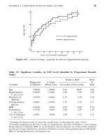
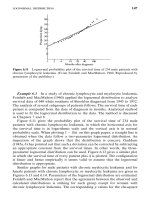
Example 14.1 Consider the ages of 71 leukemia patients — 37 responders
and 34 nonresponders (response is defined as a complete response only) —
given in Table 14.1. Figure 14.1 gives us the estimated age distributions of the
two groups. By using the Mann—Whitney U-test (or Gehan’s generalized
Wilcoxon test), we find that the difference in age between responders and
nonresponders is statistically significant (p : 0.01). In consequence, a question
may arise as to what age is critical. Can we say that patients under 50 may
have a better chance of responding than do patients over 50? To answer this
question, one can dichotomize the age data and use the chi-square test,
discussed next.
14.1.2 Chi-Square Test and Odds Ratio
The chi-square test and the odds ratio are most appropriate when the
independent variable is categorical. If the independent variable is dichotomous,
a2;2 table can be used to represent the data. Any variables that are not
dichotomous can be made so (with a loss of some information) by choos-
ing a cutoff point: for example, age less than 50 years. For multiple-
outcome events, 2;c or r;c tables can be constructed. The independent
379
Figure 14.1 Age distribution of responders and nonresponders.
variables are then examined to find which ones (in some sense) provide the
best risk associations with the dependent variable. We first consider binary
outcomes and independent variables that have two categories; that is, we set
up a 2;2 contingency table similar to Table 14.2 for each independent variable
and look for a high degree of proportionality.
The first step is to calculate the sample proportion of successes in the two
risk groups, a/C
and b/C
. Further analysis of the table is concerned with the
precision of these proportions. A standard chi-square test can be used.
380
Table 14.2 General Setup of a 2;2 Contingency Table
Risk Factor
Present (E ) Absent (E
) Total
Dependent variable
Success abR
Failure cdR
Total C
C
N
Proportion of successes (success rate) a/C
b/C
If the rates of success for the two groups E and E are exactly equal, the
expected number of patients in the ijth cell (ith row and jth column) is
E
GH
: N;
R
G
N
;
C
H
N
:
R
G
;C
H
N
(14.1.1)
For example, in the top left cell, the expected number is
E
:
R
;C
N
since the overall success rate is R
/N and there are C
individuals in the E
group. Similar expected numbers can be obtained for each of the four cells. Let
O
GH
be the number of patients observed in the ijth cell. Then the discrepancies
can be measured by the differences (O
GH
9 E
GH
). In a rough sense, the greater the
discrepancies, the more evidence we have against the null hypothesis that the
success rates are the same for the two groups. The chi-square test is based on
these discrepancies. Let
X:
G
H
(O
GH
9 E
GH
)
E
GH
(14.1.2)
Under the null hypothesis, X follows the chi-square distribution with 1 degree
of freedom (df). The hypothesis of equal success rates for groups E and E is
rejected if X 9
?
, where
?
is the 100 percentage point of the chi-square
distribution with 1 degree of freedom. An alternative way to compute X is
X:
(ad 9 bc)N
R
R
C
C
(14.1.3)
381
The odds ratio (Cornfield, 1951) is a commonly used measure of association
in 2;2 tables. The odds ratio (OR) is the ratio of two odds: the odds of success
when the risk factor is present and the odds of success when the risk factor is
absent. In terms of probabilities,
OR :
P(success "E)/P(failure " E)
P(success "E )/P(failure "E )
(14.1.4)
Using the notation in Table 14.2, P(success "E) and P(failure "E) may
be estimated by a/C
and c/C
, respectively. Similarly, P(success" E ) and
P(failure "E ) may be estimated, respectively, by b/C
and d/C
. Therefore,
the numerator and denominator of (14.1.4) may be estimated, respectively,
by
a/C
c/C
:
a
c
and
b/C
d/C
:
b
d
Consequently, the OR may be estimated by
OR
:
a/c
b/d
:
ad
bc
(14.1.5)
which is also referred to as the cross-product ratio.
Several methods are available for an interval estimate of OR: for example,
Cornfield (1956) and Woolf (1955). Cornfield’s method, which requires an
iterative procedure, is considered more accurate but more complicated than
Woolf’s method. Woolf suggests using the logarithm of OR. The standard error
of log OR
may be estimated by
SE
(log OR
) :
1
a
;
1
b
;
1
c
;
1
d
(14.1.6)
Then a 100(1 9 )% confidence interval (CI) for log OR is
log OR
< Z
?
SE
(log OR
)
The confidence interval for OR can be obtained by taking the antilog of the
confidence limits for log OR. If log OR
3
and log OR
*
are the upper and lower
382
confidence limits for log OR, e
logOR
3
and e
logOR
*
are the upper and lower
confidence limits for OR.
Notice that in (14.1.5),ifb or c is zero, OR
is undefined. If any one of the
four cell frequencies is zero, the estimated standard error in (14.1.6) is also
undefined. Should this occur, some statisticians (Haldane, 1956; Fleiss, 1979,
1981) suggest that 0.5 be added to each cell before using (14.1.5) and (14.1.6)
to solve the computational problem. However, if the cell frequencies are as
small as zero, the addition of 0.5 to each cell will substantially affect the
resulting estimate of OR and its standard error (Mantel, 1977; Miettinen,
1979). The estimates so obtained must be interpreted with caution.
An odds ratio of 1 indicates that the odds of success are the same whether
or not the risk factor is present. An odds ratio greater than 1 means that the
odds in favor of success is higher when the risk factor is present, and therefore
there is a positive association between the risk factor and success. Similarly, an
odds ratio of less than 1 signifies a negative association between the risk factor
and success. The interpretation should not be based totally on the point
estimate. A confidence interval is always more meaningful, just as in any other
estimation procedure.
The chi-square statistic in (14.1.2) may be used to test the null hypothesis
that there is no association between the risk factor and success, or H
:OR: 1.
The following example illustrates the chi-square test and odds ratio.
Example 14.2 In the study of the response rate of 71 leukemia patients
(Example 14.1), age is considered one of the possible risk variables. The
following 2;2 table is constructed.
Age :50 Age .50 Total
Response 27 10 37
Nonresponse 12 22 34
Total 39 32 71
The question is whether the response rates in the two age groups differ
significantly or whether age is associated with response.
The X value according to (14.1.3) is
X:
(594 9 120)(71)
(37)(34)(39)(32)
: 10.16
with 1 degree of freedom. Reference to Table B-2 shows that the probability of
383