Statistics for Environmental Engineers Second Edition phần 2 pot

© 2002 By CRC Press LLC
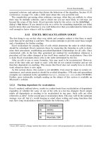
3.7 Heavy Metals. Below are 100 daily observations of wastewater influent and effluent lead (Pb)
concentration, measured as
µ
g/L, in wastewater. State your expectation for the relation
between influent and effluent and then plot the data to see whether your ideas need modifi-
cation.
Obs Inf Eff Obs Inf Eff Obs Inf Eff Obs Inf Eff
1 47 2 26 16 7 51 29 1 76 13 1
2 30 4 27 32 9 52 21 1 77 14 1
3 23 4 28 19 6 53 18 1 78 18 1
4 29 1 29 22 4 54 19 1 79 10 1
5 30 6 30 32 4 55 27 1 80 4 1
6 28 1 31 29 7 56 36 2 81 5 1
7 13 6 32 48 2 57 27 1 82 60 2
8 15 3 33 34 1 58 28 1 83 28 1
9 30 6 34 22 1 59 31 1 84 18 1
10 52 6 35 37 2 60 6 1 85 8 11
11 39 5 36 64 19 61 18 1 86 11 1
12 29 2 37 24 15 62 97 1 87 16 1
13 33 4 38 33 36 63 20 1 88 15 1
14 29 5 39 41 2 64 17 2 89 25 3
15 33 4 40 28 2 65 9 3 90 11 1
16 42 7 41 21 3 66 12 6 91 8 1
17 36 10 42 27 1 67 10 5 92 7 1
18 26 4 43 30 1 68 23 5 93 4 1
19 105 82 44 34 1 69 41 4 94 3 1
20 128 93 45 36 3 70 28 4 95 4 1
21 122 2 46 38 2 71 18 4 96 6 1
22 170 156 47 40 2 72 5 1 97 5 2
23 128 103 48 10 2 73 2 1 98 5 1

24 139 128 49 10 1 74 19 10 99 5 1
25 31 7 50 42 1 75 24 10 100 16 1
L1592_frame_C03 Page 39 Tuesday, December 18, 2001 1:41 PM
© 2002 By CRC Press LLC

4

Smoothing Data

KEY WORDS

moving average, exponentially weighted moving average, weighting factors, smooth-
ing, and median smoothing.

Smoothing is drawing a smooth curve through data in order to eliminate the roughness (scatter) that blurs
the fundamental underlying pattern. It sharpens our focus by unhooking our eye from the irregularities.
Smoothing can be thought of as a decomposition of the data. In curve fitting, this decomposition has
the general relation:

data



=



fit

+



residuals

. In smoothing, the analogous expression is:

data



=



smooth

+

rough

. Because the

smooth

is intended to be smooth (as the “fit” is smooth in curve fitting), we usually
show its points connected. Similarly, we show the

rough

(or residuals) as separated points, if we show
them at all. We may choose to show only those rough (residual) points that stand out markedly from
the smooth (Tukey, 1977).
We will discuss several methods of smoothing to produce graphs that are especially useful with time
series data from treatment plants and complicated environmental systems. The methods are well estab-
lished and have a long history of successful use in industry and econometrics. The methods are effective
and economical in terms of time and money. They are simple; they are useful to everyone, regardless
of statistical expertise. Only elementary arithmetic is needed. A computer may be helpful, but is not
needed, especially if one keeps the plot up-to-date by adding points daily or weekly as they become
available.
In statistics and quality control literature, one finds mathematics and theory that can embellish these
graphs. A formal statistical analysis, such as adding control limits, can become quite complex because
often the assumptions on which such tests are usually based are violated rather badly by environmental
data. These embellishments are discussed in another chapter.

Smoothing Methods

One method of smoothing would be to fit a straight line or polynomial curve to the data. Aside from
the computational bother, this is not a useful general procedure because the very fact that smoothing is
needed means that we cannot see the underlying pattern clearly enough to know what particular polynomial
would be useful.
The simplest smoothing method is to plot the data on a logarithmic scale (or plot the logarithm of

y

instead of

y

itself). Smoothing by plotting the moving averages (MA) or exponentially weighted moving
averages (EWMA) requires only arithmetic.
A moving average (MA) gives equal weight to a sequence of past values; the weight depends on how
many past values are to be remembered. The EWMA gives more weight to recent events and progressively
forgets the past. How quickly the past is forgotten is determined by one parameter. The EWMA will
follow the current observations more closely than the MA. Often this is desirable but this responsiveness
is purchased by a loss in smoothing.
The choice of a smoothing method might be influenced by the application. Because the EWMA forgets
the past, it may give a more realistic representation of the actual threat of the pollutant to the environment.

L1592_Frame_C04 Page 41 Tuesday, December 18, 2001 1:41 PM
© 2002 By CRC Press LLC

For example, the BOD discharged into a freely flowing stream is important the day it is discharged. A
2- or 3-day average might also be important because a few days of dissolved oxygen depression could
be disastrous while one day might be tolerable to aquatic organisms. A 30-day average of BOD could
be a less informative statistic about the threat to fish than a short-term average, but it may be needed to
assess the long-term trend in treatment plant performance.
For suspended solids that settle on a stream bed and form sludge banks, a long-term average might
be related to depth of the sludge bed and therefore be an informative statistic. If the solids do not settle,
the daily values may be more descriptive of potential damage. For a pollutant that could be ingested by
an organism and later excreted or metabolized, the exponentially weighted moving average might be a
good statistic.
Conversely, some pollutants may not exhibit their effect for years. Carcinogens are an example where
the long-term average could be important. Long-term in this context is years, so the 30-day average would
not be a particularly useful statistic. The first ingested (or inhaled) irritants may have more importance
than recently ingested material. If so, perhaps past events should be weighted more heavily than recent
events if a statistic is to relate source of pollution to present effect. Choosing a statistic with the
appropriate weighting could increase the value of the data to biologists, epidemiologists, and others who

seek to relate pollutant discharges to effects on organisms.

Plotting on a Logarithmic Scale

The top panel of Figure 4.1 is a plot of influent copper concentration at a wastewater treatment plant.
This plot emphasizes the few high values, expecially those at days 225, 250, and 340. The bottom panel
shows the same data on a logarithmic scale. Now the process behavior appears more consistent. The
low values are more evident, and the high values do not seem so extreme. The episode around day 250
still looks unusual, but the day 225 and 340 values are above the average (on the log scale) by about
the same amount that the lowest values are below average.
Are the high values so extraordinary as to deserve special attention? Or are they rogue values (outliers)
that can be disregarded? This question cannot be answered without knowing the underlying distribution
of the data. If the underlying process naturally generates data with a lognormal distribution, the high
values fit the general pattern of the data record.

FIGURE 4.1

Copper data plotted on arithmetic and logarithmic scales give a different impression about the high values.
350300250200150100500
Days
0
500
1000
10
100
1000
10000
Copper (mg/L)Copper (mg/L)

L1592_Frame_C04 Page 42 Tuesday, December 18, 2001 1:41 PM

© 2002 By CRC Press LLC

The Moving Average

Many standards for environmental quality have been written for an average of 30 consecutive days. The
language is something like the following: “Average daily values for 30 consecutive days shall not
exceed….” This is commonly interpreted to mean a monthly average, probably because dischargers
submit monthly reports to the regulatory agencies, but one should note the great difference between the
moving 30-day average and the monthly average as an effluent standard. There are only 12 monthly
averages in a year of the kind that start on the first day of a month, but there are a total of 365 moving
30-day averages that can be computed. One very bad day could make a monthly average exceed the
limit. This same single value is used to calculate 30 other moving averages and several of these might
exceed the limit. These two statistics — the strict monthly average and the 30-day moving average — have
different properties and imply different effects on the environment, although the effluent and the envi-
ronment are the same.
The length of time over which a moving average is calculated can be adjusted to represent the memory
of the environmental system as it responds to pollutants. This is done in ambient air pollution monitoring,
for example, where a short averaging time (one hour) is used for ozone.
The moving average is the simple average of the most recent

k

data points, that is, the sum of the
most recent

k

data divided by

k

:
Thus, a seven-day moving average (MA7) uses the latest seven daily values, a ten-day average (MA10)
uses 10 points, and so on. Each data point is given equal weight in computing the average.
As each new observation is made, the summation will drop one term and add another term, giving
the simple updating formula:

By smoothing random fluctuations, the moving average sharpens the focus on recent performance levels.
Figure 4.2 shows the MA7 and MA30 moving averages for some PCB data. Both moving averages help
general trends in performance show up more clearly because random variations are averaged and smoothed.

FIGURE 4.2

Seven-day and thirty-day moving averages of PCB data.
y
i
k()
1
k

y
j
i
j=i−k+1
i
∑
k, k 1,…, n+==
y
i
k() y

i −1
k()
1
k

y
i
1
k

y
i−k
–+ y
i −1
k()
1
k

y
i
y
i−k
–()+==
400350300250200
0
50
100
0
50
100

7-day moving average
30-day moving average
Observation
PCB (µg/L) PCB (µg/L)

L1592_Frame_C04 Page 43 Tuesday, December 18, 2001 1:41 PM
© 2002 By CRC Press LLC

The MA7, which is more reflective of short-term variations, has special appeal in being a weekly
average. Notice how the moving average lags behind the daily variation. The peak day is at 260, but the
MA7 peaks three to four days later (about

k

/2 days later). This does not diminish its value as a smoother,
but it does limit its value as a predictor. The longer the smoothing period (the larger

k

), the more the
average will lag behind the daily values.
The MA30 highlights long-term changes in performance. Notice the lack of response in the MA30
at day 255 when several high PCB concentrations occurred. The MA30 did not increase by very
much — only from 25

µ

g/L to about 40

µ

g/L— but it stayed at the 40

µ

g/L level for almost 30 days after
the elevated levels had disappeared. High concentrations of PCBs are not immediately harmful, but the
chemical does bioaccumulate in fish and other organisms and the long-term average is probably more
reflective of the environmental danger than the more responsive MA7.

Exponentially Weighted Moving Average

In the simple moving average, recent values and long-past values are weighted equally. For example,
the performance four weeks ago is reflected in an MA30 to the same degree as yesterday’s, although
the receiving environment may have “forgotten” the event of 4 weeks ago. The exponentially weighted
moving average (EWMA) weights the most recent event heavily, and each event going into the past
proportionately less.
The EWMA is calculated as:
where

φ

is a suitably chosen constant between 0 and 1 that determines the length of the EWMA’s memory
and how much smoothing is done.
Why do we call the EWMA an average? Because it has the property that if all the observations are
increased by some fixed amount, then the EWMA is also increased by that same amount. The weights
must add up to one (unity) for this to happen. Obviously this is true for the weights of the equally
weighted average, as well as the EWMA.
Figure 4.3 shows how the weight given to past times depends on the selected value of

φ

. The parameter

φ

indicates how much smoothing is done. As

φ

increases from 0 to 1, the smoothing increases and long-
term cycles and trends stand out more clearly. When

φ

is small, the “memory” of the EWMA is short

FIGURE 4.3

Weights for exponentially weighted moving average (EWMA).
Z
i
1
φ
–()
φ
j
y
i−j
j=0

∞
∑
i 1, 2,…==
0.0
0.2
0.4
0.6
0.8
1.0
1050
0.0
0.2
0.4
0.6
0.8
1.0
φ
= 0.1
φ
= 0.3
φ
= 0.7
φ
= 0.5
1050
W
Days in the past Days in the past
Weighting factor (1 – φ)φ
j

L1592_Frame_C04 Page 44 Tuesday, December 18, 2001 1:41 PM
© 2002 By CRC Press LLC

and the weights a few days past rapidly shrink toward zero. A value of

φ



=

0.5 to 0.3 often gives a useful
balance between smoothing and responsiveness. Values in this range will roughly approximate a sim-
ple seven-day moving average, as shown in Figure 4.4, which shows a portion of the PCB data from
Figure 4.2. Note that the EWMA (

φ



=

0.3) increases faster and recovers to normal levels faster than the
MA7. This is characteristic of EWMAs.
Mathematically, the EMWA has an infinite number of terms, but in practice only five to ten are needed
because the weight (1

−

φ

)

φ

j

rapidly approaches 0 as

j

increases. For example, if

φ



=

0.3:
The small coefficient of

y

i

−

3

shows that values more than three days into the past are essentially forgotten
because the weighting factor is small.
The EWMA can be easily updated using:
where is the EWMA at the previous sampling time and is the updated average that is computed
when the new observation of

y

i

becomes available.

Comments

Suitable graphs of data and the human mind are an effective combination. A suitable graph will often
show the smooth along with the rough. This prevents the eye from being distracted by unimportant
details. The smoothing methods illustrated here are ideal for initial data analysis (Chatfield, 1988, 1991)
and exploratory data analysis (Tukey, 1977). Their application is straightforward, fast, and easy.
The simple moving averages (7-day, 30-day, etc.) effectively smooth out random and other high-
frequency variation. The longer the averaging period, the smoother the moving average becomes and
the more slowly it reacts to changes in the underlying pattern. That is, to gain smoothness, response to
short-term change is sacrificed.
Exponentially weighted moving averages can smooth effectively while also being responsive. This is
because they give more relative weight (influence) to recent events and dilute or forget the past. The
rate of forgetting is determined by the value of the smoothing factor,

φ

. We have not tried to identify
the best value of

φ

in the EWMA. It is possible to do this by fitting time series models (Box et al., 1994;
Cryer, 1986). This becomes important if the smoothing function is used to predict future values, but it
is not necessary if we just want to clarify the general underlying pattern of variation.
An alternate to the moving average smoothers is the nonparametric median smooth (Tukey, 1977). A
median-of-3 smooth is constructed by plotting the middle value of three consecutive observations. It
can be constructed without computations and it is entirely resistant to occasional extreme values. The
computational simplicity is an insignificant advantage, however, because the moving averages are so
easy to compute.

FIGURE 4.4

Comparison of 7-day moving average and an exponentially weighted moving average with

φ



=

0.3.
300290280270260250240230
D
0
50
100

(
φ
= 0.3)
EQMA
7-day MA
Day
POB (µg/L)
Z
i
10.3–()y
i
10.3–()0.3()y
i 1–
10.3–()0.3()
2
y
i 2–
…
++ +=
Z
i
0.7y
i
0.21y
i 1–
0.063y
i 2–
0.019y
i 3–
…

+++ +=
Z
i
φ
Z
i 1–
1
φ
–()y
i
+=
Z
i 1–
Z
i
L1592_Frame_C04 Page 45 Tuesday, December 18, 2001 1:41 PM
© 2002 By CRC Press LLC
Missing values in the data series might seem to be a barrier to smoothing, but for practical purposes
they usually can be filled in using some simple ad hoc method. For purposes of smoothing to clarify
the general trend, several methods of filling in missing values can be used. The simplest is linear
interpolation between adjacent points. Other alternatives are to fill in the most recent moving average
value, or to replicate the most recent observation. The general trend will be nearly the same regardless
of the choice of method, and the user should not be unduly worried about this so long as missing values
occur only occasionally.
References
Box, G. E. P., G. M. Jenkins, and G. C. Reinsel (1994). Time Series Analysis, Forecasting and Control, 3rd
ed., Englewood Cliffs, NJ, Prentice-Hall.
Chatfield, C. (1988). Problem Solving: A Statistician’s Guide, London, Chapman & Hall.
Chatfield, C. (1991). “Avoiding Statistical Pitfalls,” Stat. Sci., 6(3), 240–268.
Cryer, J. D. (1986). Time Series Analysis, Duxbury Press, Boston.

Tukey, J. W. (1977). Exploratory Data Analysis, Reading, MA, Addison-Wesley.
Exercises
4.1 Cadmium. The data below are influent and effluent cadmium at a wastewater treatment plant.
Use graphical and smoothing methods to interpret the data. Time runs from left to right.
4.2 PCBs. Use smoothing methods to interpret the series of 26 PCB concentrations below. Time
runs from left to right.
4.3 EWMA. Show that the exponentially weighted moving average really is an average in the
sense that if a constant, say
α
= 2.5, is added to each value, the EWMA increases by 2.5.
Inf. Cd (
µµ
µµ
g/L) 2.5 2.3 2.5 2.8 2.8 2.5 2.0 1.8 1.8 2.5 3.0 2.5
Eff. Cd (
µµ
µµ
g/L) 0.8 1.0 0.0 1.0 1.0 0.3 0.0 1.3 0.0 0.5 0.0 0.0
Inf. Cd (
µµ
µµ
g/L) 2.0 2.0 2.0 2.5 4.5 2.0 10.0 9.0 10.0 12.5 8.5 8.0
Eff. Cd (
µµ
µµ
g/L) 0.3 0.5 0.3 0.3 1.3 1.5 8.8 8.8 0.8 10.5 6.8 7.8
29 62 33 189 289 135 54 120 209 176 100 137 112
120 66 90 65 139 28 201 49 22 27 104 56 35
L1592_Frame_C04 Page 46 Tuesday, December 18, 2001 1:41 PM
© 2002 By CRC Press LLC

5

Seeing the Shape of a Distribution

KEY WORDS

dot diagram, histogram, probability distribution, cumulative probability distribution,
frequency diagram.

The data in a sample have some frequency distribution, perhaps symmetrical or perhaps skewed. The
statistics (mean, variance, etc.) computed from these data also have some distribution. For example, if the
problem is to establish a 95% confidence interval on the mean, it is not important that the sample is normally
distributed because the distribution of the mean tends to be normal regardless of the sample’s distribution.
In contrast, if the problem is to estimate how frequently a certain value will be exceeded, it is essential to
base the estimate on the correct distribution of the sample. This chapter is about the shape of the distribution
of the data in the sample and not the distribution of statistics computed from the sample.
Many times the first analysis done on a set of data is to compute the mean and standard deviation. These
two statistics fully characterize a normal distribution. They do not fully describe other distributions. We
should not assume that environmental data will be normally distributed. Experience shows that stream quality
data, wastewater treatment plant influent and effluent data, soil properties, and air quality data typically do
not have normal distributions. They are more likely to have a long tail skewed toward high values (positive
skewness). Fortunately, one need not assume the distribution. It can be discovered from the data.
Simple plots help reveal the sample’s distribution. Some of these plots have already been discussed
in Chapters 2 and 3.

Dot diagrams

are particularly useful. These simple plots have been overlooked and
underused. Environmental engineering references are likely to advise, by example if not by explicit

advice, the construction of a

probability plot

(also known as the

cumulative frequency plot

). Probability
plots can be useful. Their construction and interpretation and the ways in which such plots can be
misused will be discussed.

Case Study: Industrial Waste Survey Data Analysis

The BOD (5-day) data given in Table 5.1 were obtained from an industrial wastewater survey (U.S. EPA,
1973). There are 99 observations, each measured on a 4-hr composite sample, giving six observations
daily for 16 days, plus three observations on the 17th day. The survey was undertaken to estimate the
average BOD and to estimate the concentration that is exceeded some small fraction of the time (for
example, 10%). This information is needed to design a treatment process. The pattern of variation also
needs to be seen because it will influence the feasibility of using an equalization process to reduce the
variation in BOD loading. The data may have other interesting properties, so the data presentation should
be complete, clear, and not open to misinterpretation.

Dot Diagrams

Figure 5.1 is a time series plot of the data. The concentration fluctuates rapidly with more or less equal
variation above and below the average, which is 687 mg/L. The range is from 207 to 1185 mg/L. The
BOD may change by 1000 mg/L from one sampling interval to the next. It is not clear whether the ups
and downs are random or are part of some cyclic pattern. There is little else to be seen from this plot.

L1592_Frame_C05 Page 47 Tuesday, December 18, 2001 1:42 PM
© 2002 By CRC Press LLC

A

dot diagram

shown in Figure 5.2 gives a better picture of the variability. The data have a

uniform
distribution

between 200 and 1200 mg/L. Any value within this range seems equally likely. The dot
diagrams in Figure 5.3 subdivide the data by time of day. The observed values cover the full range
regardless of time of day. There is no regular cyclic variation and no time of day has consistently high
or consistently low values.
Given the uniform pattern of variation, the extreme values take on a different meaning than if the data
were clustered around the average, as they would be in a normal distribution. If the distribution were

TABLE 5.1

BOD Data from an Industrial Survey

Date 4 am 8 am 12 N 4 pm 8 pm 12 MN

2/10 717 946 623 490 666 828
2/11 1135 241 396 1070 440 534
2/12 1035 265 419 413 961 308
2/13 1174 1105 659 801 720 454
2/14 316 758 769 574 1135 1142

2/15 505 221 957 654 510 1067
2/16 329 371 1081 621 235 993
2/17 1019 1023 1167 1056 560 708
2/18 340 949 940 233 1158 407
2/19 853 754 207 852 318 358
2/20 356 847 711 1185 825 618
2/21 454 1080 440 872 294 763
2/22 776 502 1146 1054 888 266
2/23 619 691 416 1111 973 807
2/24 722 368 686 915 361 346
2/25 1110 374 494 268 1078 481
2/26 472 671 556 —— —

Source:

U.S. EPA (1973). Monitoring Industrial Wastewater,
Washington, D.C.

FIGURE 5.1

Time series plot of the BOD data.

FIGURE 5.2

Dot diagram of the 99 BOD observations.
100806040200
0
250
500
750

1000
1250
1500
Observation (at 4-hour intervals)
BOD Concentration (mg/L)
12001000800600400200
0
1
2
3
4
5
BOD Concentration (mg/L)
Frequency

L1592_Frame_C05 Page 48 Tuesday, December 18, 2001 1:42 PM
© 2002 By CRC Press LLC

normal, the extreme values would be relatively rare in comparison to other values. Here, they are no
more rare than values near the average. The designer may feel that the rapid fluctuation with no tendency
to cluster toward one average or central value is the most important feature of the data.
The elegantly simple dot diagram and the time series plot have beautifully described the data. No
numerical summary could transmit the same information as efficiently and clearly. Assuming a “normal-
like” distribution and reporting the average and standard deviation would be very misleading.

Probability Plots

A probability plot is not needed to interpret the data in Table 5.1 because the time series plot and dot
diagrams expose the important characteristics of the data. It is instructive, nevertheless, to use these data
to illustrate how a probability plot is constructed, how its shape is related to the shape of the frequency

distribution, and how it could be misused to estimate population characteristics.
The

probability plot

, or

cumulative frequency distribution

, shown in Figure 5.4 was constructed by
ranking the observed values from small to large, assigning each value a rank, which will be denoted by

i

, and calculating the plotting position of the probability scale as

p



=



i

/

(

n



+

1), where

n

is the total
number of observations. A portion of the ranked data and their calculated plotting positions are shown
in Table 5.2. The relation

p



=



i

/

(

n

+

1) has traditionally been used by engineers. Statisticians seem to
prefer

p



=

(

i



−

0.5)

/

n

, especially when

n

is small.

1

The major differences in plotting position values
computed from these formulas occur in the tails of the distribution (high and low ranks). These differences
diminish in importance as the sample size increases.
Figure 5.4(top) is a normal probability plot of the data, so named because the probability scale (the
ordinate) is arranged in a special way to give a straight line plot when the data are normally distributed.
Any frequency distribution that is not normal will plot as a curve on the normal probability scale used
in Figure 5.4(top). The abcissa is an arithmetic scale showing the BOD concentration. The ordinate is
a cumulative probability scale on which the calculated

p

values are plotted to show the probability that
the BOD is less than the value shown on the abcissa.
Figure 5.4 shows that the BOD data are distributed symmetrically, but not in the form of a normal
distribution. The S-shaped curve is characteristic of distributions that have more observations on the tails than
predicted by the normal distribution. This kind of distribution is called “heavy tailed.” A data set that is light-
tailed (peaked) or skewed will also have an S-shape, but with different curvature (Hahn and Shapiro, 1967).
There is often no reason to make the probability plot take the form of a straight line. If a straight line
appears to describe the data, draw such a line on the graph “by eye.” If a straight line does not appear
to describe the points, and you feel that a line needs to be drawn to emphasize the pattern, draw a

FIGURE 5.3

Dot diagrams of the data for each sampling time.

1

There are still other possibilities for the probability plotting positions (see Hirsch and Stedinger, 1987). Most have the gen-
eral form of

p



=

(

i



−

a)

/

(

n



+

1

−

2a), where a is a constant between 0.0 and 0.5. Some values are: a

=

0 (Weibull), a

=

0.5
(Hazen), and a

=

0.375 (Blom).
12
4
8
12
12001000800600400200
4 am
8 am
N
pm
pm
MN

Time of Day
BOD Concentration, mg/L

L1592_Frame_C05 Page 49 Tuesday, December 18, 2001 1:42 PM
© 2002 By CRC Press LLC

smooth curve. If the plot is used to estimate the median and the 90th percentile value, a curve like
Figure 5.4(top) is satisfactory.
If a straight-line probability plot were wanted for this data, a simple arithmetic plot of

p

vs. BOD will
do, as shown by Figure 5.4(bottom). The linearity of this plot indicates that the data are uniformly
distributed over the range of observed values, which agrees with the impression drawn from the dot plots.
A probability plot can be made with a logarithmic scale on one axis and the normal probability scale
on the other. This plot will produce a straight line if the data are lognormally distributed. Figure 5.5
shows the dot diagram and normal probability plot for some data that has a lognormal distribution. The
left-hand panel shows that the logarithms are normally distributed and do plot as a straight line.
Figure 5.6 shows normal probability plots for four samples of

n



=

26 observations, each drawn at
random from a pool of observations having a mean

η



=

10 and standard deviation

σ



=

1. The sample
data in the two top panels plot neat straight lines, but the bottom panels do not. This illustrates the
difficulty in using probability plots to prove normality (or to disprove it).
Figure 5.7 is a probability plot of some industrial wastewater COD data. The ordinate is constructed
in terms of

normal scores

, also known as

rankits

. The shape of this plot is the same as if it were made

TABLE 5.2

Probability Plotting Positions for the

n



=

99

Values in Table 5.1

BOD Value
(mg

//
//

L)
Rank

i

Plotting Position

p

= 1

//

//

(

n

+ 1)



207 1 1

/

100

=

0.01
221 2 0.02
223 3 0.03
235 4 0.04
………
1158 96 0.96
1167 97 0.97
1174 98 0.98
1185 99 0.99

FIGURE 5.4

Probability plots of the uniformly distributed BOD data. The top panel is

a normal probability plot

. The
ordinate is scaled so that normally distributed data would plot as a straight line. The bottom panel is scaled so the BOD
data plot as a straight line. These BOD data are not normally distributed. They are uniformly distributed.
1200700200
.999
.99
.95
.80
.50
.20
.05
.01
.001
1.0
0.5
0.0
BOD Concentration (mg/L)
Probabiltity BOD
less than Abscissa Value
Probabiltity BOD
less than Abscissa Value

L1592_Frame_C05 Page 50 Tuesday, December 18, 2001 1:42 PM
© 2002 By CRC Press LLC

FIGURE 5.5

The logarithms of the lognormal data on the right will plot as a straight line on a normal probability plot
(left-hand panel).

FIGURE 5.6

Normal probability plots, each constructed with

n



=

26 observations drawn at random from a normal
distribution with

η



=

10 and

σ

=

1. Notice the difference in the range of values in the four samples.

FIGURE 5.7

Probability plot constructed in terms of normal
order scores, or

rankits

. The ordinate is the normal distribution
measured in standard deviations; 1 rankit

=

1 standard devi-
ation. Rankit

=

0 is the median (50th percentile).
Probabitlity
.999
.99
.95
.80
.50
.20

.05
.01
.001
432106040200
log (Concentration) Concentration
log-transformed data have a
normal distribution
Lognormal distribution
1211109812111098
111098712111098
ProbabilityProbability
0.999
0.99
0.95
0.80
0.50
0.20
0.05
0.01
0.001
0.999
0.99
0.95
0.80
0.50
0.20
0.05
0.01
0.001
500 1000 2000 5000 10000

COD Concentration (mg/L)
Rankits
3
2
1
0
-1
-2
-3

L1592_Frame_C05 Page 51 Tuesday, December 18, 2001 1:42 PM
© 2002 By CRC Press LLC

on normal probability paper. Normal scores or rankits can be generated in many computer software
packages (such as Microsoft Excel) and can be looked up in standard statistical tables (Sokal and Rohlf,
1969). This is handy because some graphics programs do not draw probability plots. Another advantage
of using rankits is that linear regression can be done on the rankit scores (see the example of censored
data analysis in Chapter 15).

The Use and Misuse Probability Plots

Engineering texts often suggest estimating the mean and sample standard deviations of a sample from
a probability plot, saying that the mean is located at

p



=

50% on a normal probability graph and the
standard deviation is the distance from

p



=

50% to

p



=

84.1% (or, because of symmetry, from

p



=

15.9%
to

p

=

50%). These graphical estimates are valid only when the data are normally distributed. Because
few environmental data sets are normally distributed, this graphical estimation of the mean and standard
deviation is not recommended. A probability plot is useful, however, to estimate the median (

p



=

50%)
and to read directly any percentile of special interest.
One way that probability plots are misused is to make the graphical estimates of sample statistics
when the distribution is not normal. For example, if the data are lognormally distributed,

p



=

50% is the
median and not the arithmetic mean, and the distance from

p

=

50% to

p



=

84.1% is not the sample
standard deviation. If the data have a uniform distribution, or any other symmetrical distribution,

p



=

50%
is the median

and

the average, but the standard deviation cannot be read from the probability plot.

Randomness and Independence

Data can be normally distributed without being random or independent. Furthermore, randomness and
independence cannot be perceived or proven using a probability plot. This plot does not provide any
information regarding serial dependence or randomness, both of which may be more critical than
normality in the statistical analysis.
The histogram of the 52 weekly BOD loading values plotted on the right side of Figure 5.8 is sym-
metrical. It looks like a normal distribution and the normal probability plot will be a straight line. It
could be said therefore that the sample of 52 observations is normally distributed. This characterization
is uninteresting and misleading because the data are not randomly distributed about the mean and there
is a strong trend with time (i.e., serial dependence). The time series plot, Figure 5.8, shows these important
features. In contrast, the probability plot and dot plot, while excellent for certain purposes, obscure these
features. To be sure that all important features of the data are revealed, a variety of plots must be used,
as recommended in Chapter 3.

FIGURE 5.8

This sample of 52 observations will give a linear normal probability plot, but such a plot would hide the
important time trend and the serial correlation.
504030201000
Week
Average BOD Load
(1000 kg/wk)
0
10000
20000
30000
40000
50000
60000

L1592_Frame_C05 Page 52 Tuesday, December 18, 2001 1:42 PM

© 2002 By CRC Press LLC

Comments

We are almost always interested in knowing the shape of a sample’s distribution. Often it is important
to know whether a set of data is distributed symmetrically about a central value, or whether there is a
tail of data toward a high or a low value. It may be important to know what fraction of time a critical
value is exceeded.
Dot plots and probability plots are useful graphical tools for seeing the shape of a distribution. To
avoid misinterpreting probability plots, use them only in conjunction with other plots. Make dot diagrams
and, if the data are sequential in time, a time series plot. Sometimes these graphs provide all the important
information and the probability plot is unnecessary.
Probability plots are convenient for estimating percentile values, especially the median (50th percen-
tile) and extreme values. It is not necessary for the probability plot to be a straight line to do this. If it
is straight, draw a straight line. But if it is not straight, draw a smooth curve through the plotted points
and go ahead with the estimation.
Do not use probability plots to estimate the mean and standard deviation except in the very special
case when the data give a linear plot on normal probability paper. This special case is common in
textbooks, but rare with real environmental data. If the data plot as a straight line on log-probability
paper, the 50th percentile value is not the mean (it is the geometric mean) and there is no distance that
can be measured on the plot to estimate the standard deviation.
Probability plots may be useful in discovering the distribution of the data in a sample. Sometimes the
analysis is not clear-cut. Because of random sampling variation, the curve can have a substantial amount
of “wiggle” when the data actually are normally distributed. When the number of observations approaches
50, the shape of the probability distribution becomes much more clear than when the sample is small
(for example, 20 observations). Hahn and Shapiro (1967) point out that:

1.

The variance of points in the tails (extreme low or high plotted values) will be larger than

that of points at the center of the distribution. Thus, the relative linearity of the plot near the
tails of the distribution will often seem poorer than at the center even if the correct model
for the probability density distribution has been chosen.
2. The plotted points are ordered and hence are not independent. Thus, we should not expect
them to be randomly scattered about a line. For example, the points immediately following
a point above the line are also likely to be above the line. Even if the chosen model is correct,
the plot may consist of a series of successive points (known as runs) above and below the line.
3. A model can never be proven to be adequate on the basis of sample data. Thus, the probability
of a small sample taken from a near-normal distribution will frequently not differ appreciably
from that of a sample from a normal distribution.
If the data have positive skew, it is often convenient to use graph paper that has a log scale on one
axis and a normal probability scale on the other axis. If the logarithms of the data are normally distributed,
this kind of graph paper will produce a straight-line probability plot. The log scale may provide a
convenient scaling for the graph even if it does not produce a straight-line plot; for example, when the
data are bacterial counts that range from 10 to 100,000.

References

Hahn, G. J. and S. S. Shapiro (1967).

Statistical Methods for Engineers,

New York, John Wiley.
Hirsch, R. M. and J. D. Stedinger (1987). “Plotting Positions for Historical Floods and Their Precision,”

Water
Resources Research,

23(4), 715–727.
Mage, D. T. (1982). “An Objective Graphical Method for Testing Normal Distributional Assumptions Using

Probability Plots,”

Am. Statistician,

36, 116–120.

L1592_Frame_C05 Page 53 Tuesday, December 18, 2001 1:42 PM
© 2002 By CRC Press LLC

Sokal, R. R. and F. J. Rohlf (1969). Biometry: The Principles and Practice of Statistics in Biological Research,
New York, W.H. Freeman & Co.
U.S. EPA (1973). Monitoring Industrial Wastewater, Washington, D.C.
Exercises
5.1 Normal Distribution. Graphically determine whether the following data could have come
from a normal distribution.
5.2 Flow and BOD. What is the distribution of the weekly flow and BOD data in Exercise 3.3?
5.3 Histogram. Plot a histogram for these data and describe the distribution.
5.4 Wastewater Lead. What is the distribution of the influent lead and the effluent lead data in
Exercise 3.7?
Data Set A 13 21 13 18 27 16 17 18 22 19
15 21 18 20 23 25 5 20 20 21
Data Set B 22 24 19 28 22 23 20 21 25 22
18 21 35 21 36 24 24 23 23 24
0.02 0.18 0.34 0.50 0.65 0.81
0.04 0.20 0.36 0.51 0.67 0.83
0.06 0.22 0.38 0.53 0.69 0.85
0.08 0.24 0.40 0.55 0.71 0.87
0.10 0.26 0.42 0.57 0.73 0.89
0.12 0.28 0.44 0.59 0.75 0.91
0.14 0.30 0.46 0.61 0.77 0.93

0.16 0.32 0.48 0.63 0.79 0.95
L1592_Frame_C05 Page 54 Tuesday, December 18, 2001 1:42 PM
© 2002 By CRC Press LLC

6

External Reference Distributions

KEY WORDS

histogram, reference distribution, moving average, normal distribution, serial corre-
lation

,



t

distribution.

When data are analyzed to decide whether conditions are as they should be, or whether the level of some
variable has changed, the fundamental strategy is to compare the current condition or level with an
appropriate reference distribution. The reference distribution shows how things should be, or how they
used to be. Sometimes an external reference distribution should be created, instead of simply using one
of the well-known and nicely tabulated statistical reference distributions, such as the normal or

t

distri-

bution. Most statistical methods that rely upon these distributions assume that the data are random,
normally distributed, and independent. Many sets of environmental data violate these requirements.
A specially constructed reference distribution will not be based on assumptions about properties of
the data that may not be true. It will be based on the data themselves, whatever their properties. If
serial correlation or nonnormality affects the data, it will be incorporated into the external reference
distribution.
Making the reference distribution is conceptually and mathematically simple. No particular knowledge
of statistics is needed, and the only mathematics used are counting and simple arithmetic. Despite this
simplicity, the concept is statistically elegant, and valid judgments about statistical significance can be
made.

Constructing an External Reference Distribution

The first 130 observations in Figure 6.1 show the natural background pH in a stream. Table 6.1 lists the
data. Suppose that a new effluent has been discharged to the stream and someone suggests it is depressing
the stream pH. A survey to check this has provided ten additional consecutive measurements: 6.66, 6.63,
6.82, 6.84, 6.70, 6.74, 6.76, 6.81, 6.77, and 6.67. Their average is 6.74. We wish to judge whether this
group of observations differs from past observations. These ten values are plotted as open circles on the
right-hand side of Figure 6.1. They do not appear to be unusual, but a careful comparison should be
made with the historical data.
The obvious comparison is the 6.74 average of the ten new values with the 6.80 average of the previous
130 pH values. One reason not to do this is that the standard procedure for comparing two averages,
the

t

-test, is based on the data being independent of each other in time. Data that are a time series, like
these pH data, usually are not independent. Adjacent values are related to each other. The data are serially
correlated (autocorrelated) and the

t

-test is not valid unless something is done to account for this
correlation. To avoid making any assumption about the structure of the data, the average of 6.74 should
be compared with a reference distribution for averages of sets of ten consecutive observations.
Table 6.1 gives the 121 averages of ten consecutive observations that can be calculated from the
historical data. The ten-day moving averages are plotted in Figure 6.2. Figure 6.3 is a reference distri-
bution for these averages. Six of the 121 ten-day averages are as low as 6.74. About 95% of the ten-
day averages are larger than 6.74. Having only 5% of past ten-day averages at this level or lower indicates
that the river pH may have changed.

L1592_frame_C06 Page 55 Tuesday, December 18, 2001 1:43 PM
© 2002 By CRC Press LLC

TABLE 6.1

Data Used to Plot Figure 6.1 and the Associated External Reference Distributions

6.79 6.84 6.85 6.47 6.67 6.76 6.75 6.72 6.88 6.83 6.65 6.77 6.92 6.73 6.94 6.84 6.71
6.88 6.66 6.97 6.63 7.06 6.55 6.77 6.99 6.70 6.65 6.87 6.89 6.92 6.74 6.58 6.40 7.04
6.95 7.01 6.97 6.78 6.88 6.80 6.77 6.64 6.89 6.79 6.77 6.86 6.76 6.80 6.80 6.81 6.81
6.80 6.90 6.67 6.82 6.68 6.76 6.77 6.70 6.62 6.67 6.84 6.76 6.98 6.62 6.66 6.72 6.96
6.89 6.42 6.68 6.90 6.72 6.98 6.74 6.76 6.77 7.13 7.14 6.78 6.77 6.87 6.83 6.84 6.77
6.76 6.73 6.80 7.01 6.67 6.85 6.90 6.95 6.88 6.73 6.92 6.76 6.68 6.79 6.93 6.86 6.87
6.95 6.73 6.59 6.84 6.62 6.77 6.53 6.94 6.91 6.90 6.75 6.74 6.74 6.76 6.65 6.72 6.87
6.92 6.98 6.70 6.97 6.95 6.94 6.93 6.80 6.84 6.78 6.67

Note:

Time runs from left to right.

FIGURE 6.1

Time series plot of the pH data with the moving average of ten consecutive values.

FIGURE 6.2

Ten-day moving averages of pH.

FIGURE 6.3

External reference distribution for ten-day moving averages of pH.
6.2
6.4
6.6
6.8
7.0
7.2
pH
Days
1501251007550250
1501251007550250
6.70
6.75
6.80
6.85
6.90
pH (-10 day MA)
Observation
6.76 6.8 6.84 6.88

0
5
10
15
Frequency
10-day Moving Average of pH

L1592_frame_C06 Page 56 Tuesday, December 18, 2001 1:43 PM
© 2002 By CRC Press LLC

Using a Reference Distribution to Compare Two Mean Values

Let the situation in the previous example change to the following. An experiment to evaluate the effect
of an industrial discharge into a treatment process consists of making 10 observations consecutively
before any addition and 10 observations afterward. We assume that the experiment is not affected by
any transients between the two operating conditions. The average of 10 consecutive pre-discharge samples
was 6.80, and the average of the 10 consecutive post-discharge samples was 6.86. Does the difference
of 6.80

−

6.86

=



−

0.06 represent a significant shift in performance?

A reference distribution for the difference between batches of 10 consecutive samples is needed.
There are 111 differences of MA10 values that are 10 days apart that can be calculated from the data in
Table 6.1. For example, the difference between the averages of the 10th and 20th batches is 6.81

−

6.76

=

0.05. The second value is the difference between the 11th and 21st is 6.74

−

6.80

=



−

0.06. Figure 6.4
is the reference distribution of the 111 differences of batches of 10 consecutive samples. A downward
difference as large as

−

0.06 has occurred frequently. We conclude that the new condition is not different
than the recent past.

Looking at the 10-day moving averages suggests that the stream pH may have changed. Looking at
the differences in averages indicates that a noteworthy change has not occurred. Looking at the differences
uses more information in the data record and gives a better indication of change.

Using a Reference Distribution for Monitoring

Treatment plant effluent standards and water quality criteria are usually defined in terms of 30-day averages
and 7-day averages. The effluent data themselves typically have a lognormal distribution and are serially
correlated. This makes it difficult to derive the statistical properties of the 30- and 7-day averages. Fortu-
nately, if historical data are readily available at all treatment plants and we can construct external reference
distributions, not only for 30- and 7-day averages, but also for any other statistics of interest.
The data in this example are effluent 5-day BOD measurements that have been made daily on 24-hour
flow-weighted composite samples from an activated sludge treatment plant. We realize that BOD data
are not timely for process control decisions, but they can be used to evaluate whether the plant has been
performing at its normal level or whether effluent quality has changed. A more complete characterization
of plant performance would include reference distributions for other variables, such as suspended solids,
ammonia, and phosphorus.
A long operating record was used to generate the top histogram in Figure 6.5. From the operator’s
log it was learned that many of the days with high BOD had some kind of assignable problem. These
days were defined as unstable performance, the kind of performance that good operation could elimi-
nate. Eliminating these poor days from the histogram produces the target stable performance shown by
the reference distribution in the bottom panel of Figure 6.5. “Stable” is the kind of performance of which

FIGURE 6.4

External reference distribution for differences of 10-day moving averages of pH.
0
10
20
Frequency

Difference of 10-day Moving
Averages10 Days Apart
-0.12 -0.08 -0.04 0 0.04 0.08
3%
5% 5%
6%

L1592_frame_C06 Page 57 Tuesday, December 18, 2001 1:43 PM
© 2002 By CRC Press LLC

the plant is capable over long stretches of time (Berthouex and Fan, 1986). This is the reference distribution
against which new daily effluent measurements should be compared when they become available, which
is five or six days after the event in the case of BOD data.
If the 7-day moving average is used to judge effluent quality, a reference distribution is required for this
statistic. The periods of stable operation were used to calculate the 7-day moving averages that produce
the reference distribution shown in Figure 6.6 (top). Figure 6.6 (bottom) is the reference distribution of
30-day moving averages for periods of stable operation. Plant performance can now be monitored by
comparing, as they become available, new 7- or 30-day averages against these reference distributions.

FIGURE 6.5

External reference distributions for effluent 5-day BOD (mg/L) for the complete record and for the stable
operating conditions.

FIGURE 6.6

External reference distributions for 7- and 30-day moving averages of effluent 5-day BOD during periods
of stable treatment plant operation.
0 5 10 15 20 25 30 35
0

5
10
15
0
5
10
15
PercentagePercentage
All days
Stable operation
5-day BOD (mg/L)
0.20
0
5
10
15
0
5
10
15
PercentagePercentage
Effluent BOD (mg/L)
7-day moving average
30-day moving average
3 5 7 9 11 13 15 17

L1592_frame_C06 Page 58 Tuesday, December 18, 2001 1:43 PM
© 2002 By CRC Press LLC

Setting Critical Levels

The reference distribution shows at a glance which values are exceptionally high or low. What is meant
by “exceptional” can be specified by setting critical decision levels that have a specified probability
value. For example, one might specify exceptional as the level that is exceeded

p

percent of the time.
The reference distribution for daily observations during stable operation (bottom panel in Figure 6.5)
is based on 1150 daily values representing stable performance. The critical upper 5% level cut is a BOD
concentration of 33 mg/L. This is found by summing the frequencies, starting from the highest BOD
observed during stable operation, until the accumulated percentage equals or exceeds 5%. In this case, the
probability that the BOD is 20 is P(BOD

=

20)

=

0.8%. Also, P(BOD

=

19)

=

0.8%, P(BOD

=

18)

=

1.6%,
and P(BOD

=

17)

=

1.6%. The sum of these percentages is 4.8%. So, as a practical matter, we can say
that the BOD exceeds 16 mg/L only about 5% of the time when operation is stable.
Upper critical levels can be set for the MA(7) reference distribution as well. The probability that a
7-day MA(7) of 14 mg/L or higher will occur when the treatment plant is stable is 4%. An MA(7)
greater than 13 mg/L serves warning that the process is performing poorly and may be upset. By definition,
5% of such warnings will be false alarms. A two-level warning system could be devised, for example,
by using the upper 1% and the upper 5% levels. The upper 1% level, which is about 16 mg/L, is a signal
that something is almost certainly wrong; it will be a false in only 1 out of 100 alerts.
There is a balance to be found between having occasional false alarms and no false alarms. Setting
a warning at the 5% level, or perhaps even at the 10% level, means that an operator is occasionally sent
to look for a problem when none exists. But it also means that many times a warning is given before a
problem becomes too serious and on some of these occasions action will prevent a minor upset from
becoming more serious. An occasional wild goose chase is the price paid for the early warnings.

Comments

Consider why the warning levels were determined empirically instead of by calculating the mean and
standard deviation and then using the normal distribution. People who know some statistics tend to think
of the bell-shaped, symmetrical normal distribution when they hear that “the mean is X and the standard
deviation is Y.” The words “mean” and “standard deviation” create an image of approximately 95% of
the values falling within two standard deviations of the mean.
A glance at Figure 6.6 reveals why this is an inappropriate image for the reference distribution of
moving averages. The distributions are not symmetrical and, furthermore, they are truncated. These
characteristics are especially evident in the MA(30) distribution. By definition, the effluent BOD values
are never very high when operation is stable, so MA cannot take on certain high values. Low values of
the MA do not occur because the effluent BOD cannot be less than zero and values less than 2 mg/L
were not observed. The normal distribution, with its finite probability of values occurring far out on the
tails of the distribution (and even into negative values), would be a terrible approximation of the reference
distribution derived from the operating record.
The reference distribution for the daily values will always give a warning before the MA does. The
MA is conservative. It flattens one-day upsets, even fairly large ones, and rolls smoothly through short
intervals of minor disturbances without giving much notice. The moving average is like a shock absorber
on a car in that it smooths out the small bumps. Also, just as a shock absorber needs to have the right
stiffness, a moving average needs to have the right length of memory to do its job well. A 30-day MA is
an interesting statistic to plot only because effluent standards use a 30-day average, but it is too sluggish
to usefully warn of trouble. At best, it can confirm that trouble has existed. The seven-day average is more
responsive to change and serves as a better warning signal. Exponentially weighted moving averages (see
Chapter 4) are also responsive and reference distributions can be constructed for them as well.
Just as there is no reason to judge process performance on the basis of only one variable, there is no
reason to select and use only one reference distribution for any particular single variable. One statistic
and its reference distribution might be most useful for process control while another is best for judging

L1592_frame_C06 Page 59 Tuesday, December 18, 2001 1:43 PM
© 2002 By CRC Press LLC

compliance. Some might give early warnings while others provide confirmation. Because reference
distributions are easy to construct and use, they should be plentiful and prominent in the control room.

References

Berthouex, P. M. and W. G. Hunter, (1983). “How to Construct a Reference Distribution to Evaluate Treatment
Plant Performance,”

J. Water Poll. Cont. Fed.,

55, 1417–1424.
Berthouex, P. M. and R. Fan (1986). “Treatment Plant Upsets: Causes, Frequency, and Duration,”

J. Water
Poll. Cont. Fed.,

58, 368–375.

Exercises

6.1

BOD Tests. The table gives 72 duplicate measurements of wastewater effluent 5-day BOD
measured at 2-hour intervals. (a) Develop reference distrbutions that would be useful to the
plant operator. (b) Develop a reference distribution for the difference between duplicates that
would be useful to the plant chemist.

6.2

Wastewater Effluent TSS. The histogram shows one year’s total effluent suspended solids

data (

n



=

365) for a wastewater treatment plant (data from Exercise 3.5). The average TSS
concentration is 21.5 mg/L. (a) Assuming the plant performance will continue to follow this
pattern, indicate on the histogram the upper 5% and upper 10% levels for out-of-control
performance. (b) Calculate (approximately) the annual average effluent TSS concentration if
the plant could eliminate all days with TSS

>

upper 10% level specified in (b).

Time BOD (mg/L) Time BOD (mg/L) Time BOD (mg/L) Time BOD (mg/L)

2 185 193 38 212 203 74 124 118 110 154 139
4 116 119 40 167 158 76 166 157 112 142 129
6 158 156 42 116 118 78 232 225 114 142 137
8 185 181 44 122 129 80 220 207 116 157 174
10 140 135 46 119 116 82 220 214 118 196 197
12 179 174 48 119 124 84 223 210 120 136 124
14 173 169 50 172 166 86 133 123 122 143 138
16 119 119 52 106 105 88 175 156 124 116 108
18 119 116 54 121 124 90 145 132 126 128 123
20 113 112 56 163 162 92 139 132 128 158 161

22 116 115 58 148 140 94 148 130 130 158 150
24 122 110 60 184 184 96 133 125 132 194 190
26 161 171 62 175 172 98 190 185 134 158 148
28 110 116 64 172 166 100 187 174 136 155 145
30 176 166 66 118 117 102 190 171 138 137 129
32 197 191 68 91 98 104 115 102 140 152 148
34 167 165 70 115 108 106 136 127 142 140 127
36 179 178 72 124 119 108 154 141 144 125 113
0
20
40
60
80
Frequency
0 5 10 15 20 25 30 35 40 45 50 55 60 65 70 75
Final Effluent Total Susp. Solids

L1592_frame_C06 Page 60 Tuesday, December 18, 2001 1:43 PM
© 2002 By CRC Press LLC

7

Using Transformations

KEY WORDS

antilog, arcsin, bacterial counts, Box-Cox transformation, cadmium, confidence inter-
val, geometric mean, transformations, linearization, logarithm, nonconstant variance, plankton counts,
power function, reciprocal, square root, variance stabilization.

There is usually no scientific reason why we should insist on analyzing data in their original scale of
measurement. Instead of doing our analysis on

y

it may be more appropriate to look at log(

y

), 1

/

y

,
or some other function of

y

. These re-expressions of

y

are called transformations. Properly used trans-
formations eliminate distortions and give each observation equal power to inform.
Making a transformation is not cheating. It is a common scientific practice for presenting and inter-
preting data. A pH meter reads in logarithmic units, and not in hydrogen ion concen-
tration units. The instrument makes a data transformation that we accept as natural. Light absorbency
is measured on a logarithmic scale by a spectrophotometer and converted to a concentration with the

aid of a calibration curve. The calibration curve makes a transformation that is accepted without
hesitation. If we are dealing with bacterial counts,

N

, we think just as well in terms of log(

N

) as

N

itself.
There are three technical reasons for sometimes doing the calculations on a transformed scale: (1) to
make the spread equal in different data sets (to make the variances uniform); (2) to make the distribution
of the residuals normal; and (3) to make the effects of treatments additive (Box et al., 1978).

1

Equal
variance means having equal spread at the different settings of the independent variables or in the different
data sets that are compared. The requirement for a normal distribution applies to the measurement errors
and not to the entire sample of data. Transforming the data makes it possible to satisfy these requirements
when they are not satisfied by the original measurements.

Transformations for Linearization

Transformations are sometimes used to obtain a straight-line relationship between two variables. This
may involve, for example, using reciprocals, ratios, or logarithms. The left-hand panel of Figure 7.1 shows

the exponential growth of bacteria. Notice that the variance (spread) of the counts increases as the population
density increases. The right-hand panel shows that the data can be described by a straight line when plotted
on a log scale. Plotting on a log scale is equivalent to making a log transformation of the data.
The important characteristic of the original data is the nonconstant variance, not nonlinearity. This is
a problem when the curve or line is fitted to the data using regression. Regression tries to minimize the
distance between the data points and the line described by the model. Points that are far from the line
exert a strong effect because the regression mathematics wants to reduce the square of this distance. The result
is that the precisely measured points at time

t



=

1 will have less influence on the position of the regression
line than the poorly measured data at

t



=

3. This gives too much influence to the least reliable data. We
would prefer for each data point to have about the same amount of influence on the location of the line.
In this example, the log-transformed data have constant variance at the different population levels. Each data

1

For example, if

y



=



x

a

z

b

, a log transformation gives log

y



=



a

log

x

+

b

log

z

. Now the effects of factors

x

and

z

are additive.
See Box et al. (1978) for an example of how this can be useful.
y,
pH log
10
H
+
[]–=

L1592_frame_C07.fm Page 61 Tuesday, December 18, 2001 1:44 PM

© 2002 By CRC Press LLC

value has roughly equal weight in determining the position of the line. The log transformation is used to
achieve this equal weighting and not because it gives a straight line.
A word of warning is in order about using transformations to obtain linearity. A transformation can
turn a good situation into a bad one by distorting the variances and making them unequal (see Chapter 45).
Figure 7.2 shows a case where the constant variance of the original data is destroyed by an inappropriate
logarithmic transformation.
In the examples above it was easy to check the variances at the different levels of the independent variables
because the measurements had been replicated. If there is no replication, this check cannot be made. This
is only one reason why replication is always helpful and why it is recommended in experimental and moni-
toring work.
Lacking replication, should one assume that the variances are originally equal or unequal? Sometimes
the nature of the measurement process gives a hint as to what might be the case. If dilutions or concentrations
are part of the measurement process, or if the final result is computed from the raw measurements, or
if the concentration levels are widely different, it is not unusual for the variances to be unequal and to
be larger at high levels of the independent variable. Biological counts frequently have nonconstant
variance. These are not justifications to make transformations indiscriminately. Do not avoid making
transformations, but use them wisely and with care.

Transformations to Obtain Constant Variance

When the variance changes over the range of experimental observations, the variance is said to be non-
constant, or unstable. Common situations that tend to create this pattern are (1) measurements that involve
making dilutions or other steps that introduce multiplicative errors, (2) using instruments that read out on
a log scale which results in low values being recorded more precisely than high values, and (3) biological
counts. One of the transformations given in Table 7.1 should be suitable to obtain constant variance.

FIGURE 7.1

An example of how a transformation can create constant variance. Constant variance at all levels is important
so each data point will carry equal weight in locating the position of the fitted curve.

FIGURE 7.2

An example of how a transformation could create nonconstant variance.
43210
43210
0
200
400
600
800
1000
1200
MPN count
Time Time
10
100
1000
10000
121086420 121086420
0
20
40
60
80
100
1
10

100
Concentration

L1592_frame_C07.fm Page 62 Tuesday, December 18, 2001 1:44 PM
© 2002 By CRC Press LLC

The effect of square root and logarithmic transformations is to make the larger values less important
relative to the small ones. For example, the square root converts the values (0, 1, 4) to (0, 1, 2). The 4,
which tends to dominate on the original scale, is made relatively less important by the transformation.
The log transformation is a stronger transformation than the square root transformation. “Stronger” means
that the range of the transformed variables is relatively smaller for a log transformation that for the square
root. When the sample contains some zero values, the log transformation is

x



=

log(

y



+



c

), where

c

is a
constant. Usually the value of

c

is arbitrarily chosen to be 1 or 0.5. The larger the value of

c

, the less severe
the transformation. Similarly, for square root transformations, is less severe than
The arcsin transformation is used for decimal fractions and is most useful when the sample includes values
near 0.00 and 1.00. One application is in bioassys where the data are fractions of organisms showing an effect.

Example 7.1

Twenty replicate samples from five stations were counted for plankton, with the results given in
Table 7.2. The computed averages and variances are in Table 7.3. The computed means and variance
on the original data show that variance is not uniform; it is ten times larger at station 5 than at
station 1. Also, the variance increases as the average increases and seems to be proportional to
This indicates that a square root transformation may be suitable. Because most of the counts

TABLE 7.1

Transformations that are Useful to Obtain Uniform Variance

Condition Replace

y

by

σ

uniform over range of

y

no transformation needed


x



=

1

/

y


all

y



>

0

x



=

log(

y

)
some

y



=

0

x



=

log(

y



+



c

)
all

y



>

0
some

y



<

0

p



=

ratio or percentage

x



=

arcsin

Source:

Box, G. E. P., W. G. Hunter, and J. S. Hunter (1978).

Statistics for Experimenters:
An Introduction to Design, Data Analysis, and Model Building,

New York, Wiley Interscience.

TABLE 7.2

Plankton Counts on 20 Replicate Water Samples from Five Stations in a Reservoir

Station 1 0 2 1 0 0 1 1 0 1 1 0 2 1 0 0 23011
Station 2 3 1 1 1 4 0 1 4 3 3 5 3 2 2 1 12220
Station 3 6 1 5 7 4 1 6 5 3 3 5 3 4 3 8 42242
Station 4 7 2 6 9 5 2 7 6 4 3 5 3 6 4 8 52341
Station 5 12 7 10 15961311871081181496795

Source:

Elliot, J. (1977).

Some Methods for the Statistical Analysis of Samples of Benthic Invertebrates,

2nd ed.,
Ambleside, England, Freshwater Biological Association.

TABLE 7.3

Statistics Computed from the Data in Table 7.2

Station 1 2 4 5 6

Untransformed data

Transformed
= 0.85 2.05 3.90 4.60 9.25
= 0.77 1.84 3.67 4.78 7.57
= 1.10 1.54 2.05 2.20 3.09
= 0.14 0.20 0.22 0.22 0.19
σ
y
2
∝
σ
y
3/2
∝ x 1/ y=
σ
y
σ
2
y>()∝
σ
y
1/2
∝ xy=
xyc+=
σ
2
y> p
xyc+=
y
s
y

2
x
s
x
2
yc+ y.
s
y
2
y.

L1592_frame_C07.fm Page 63 Tuesday, December 18, 2001 1:44 PM

are small, the transform used was Figure 7.3 shows the distribution of the original and
the transformed data. The transformed distributions are more symmetrical and normal-like than the
originals. The variances computed from the transformed data are uniform.

Example 7.2

Table 7.4 shows eight replicate measurements of bacterial density that were made at three
locations to study the spatial pattern of contamination in an estuary. The data show that and
that

s

increases in proportion to Table 7.1 suggests a logarithmic transformation. The improvement
due to the log transformation is shown in Table 7.4. Note that the transformation could be done
using either log

e

or log

10

because they differ by only a constant (log

e



=

2.303 log

10

).

FIGURE 7.3

Original and transformed plankton counts.

TABLE 7.4

Eight Replicate Measurements on Bacteria at Three Sampling Stations

y

==
==

Bacteria/100 mL

x



==
==

log

10

(Bacteria/100 mL)
123123

27 225 1020 1.431 2.352 3.009
11 99 136 1.041 1.996 2.134
48 41 317 1.681 1.613 2.501
36 60 161 1.556 1.778 2.207
120 190 130 2.079 2.279 2.114
85 240 601 1.929 2.380 2.779
18 90 760 1.255 1.954 2.889
130 112 240 2.144 2.049 2.380

=

59.4 132 420.6

=

1.636 2.050 2.502


=

2156 5771 111,886

=

0.151 0.076 0.124
0
10
0
10
0
10
0
10
0
10
161284432100
Station 1
Station 2

Station 3
Station 4
Station 5
Plankton Count Count + 0.5
Frequency
y
x
s
y
2
s
x
2
y 0.5+ .
s
2
y>
y.

L1592_frame_C07.fm Page 64 Tuesday, December 18, 2001 1:44 PM
© 2002 By CRC Press LLC