Statistics for Environmental Engineers Second Edition phần 4 pot

© 2002 By CRC Press LLC
The transformation equations to convert these into estimates of the mean and variance of the
untransformed y’s are:
Substituting the parameter estimates and gives:
The Delta-Lognormal Distribution
The delta-lognormal method estimates the mean of a sample of size n as a weighted average of n
c
replaced
censored values and n – n
c
uncensored lognormally distributed values. The Aitchison method (1955, 1969)
assumes that all censored values are replaced by zeros (D
= 0) and the noncensored values have a lognormal
distribution. Another approach is to replace censored values by the detection limit (D
= MDL) or by some
value between zero and the MDL (U.S. EPA, 1989; Owen and DeRouen, 1980).
The estimated mean is a weighted average of the mean of n
c
values that are assigned value D and the
mean of the n – n
c
fully measured values that are assumed to have a lognormal distribution with mean
η
x
and variance .
where and are the estimated mean and variance of the log-transformed noncensored values.
This method gives results that agree well with Cohen’s method, but it is not consistently better than
Cohen’s method. One reason is that the user is required to assume that all censored values are located
at a single value, which may be zero, the limit of detection, or something in between.
Comments
The problem of censored data starts when an analyst decides not to report a numerical value and instead

reports “not detected.” It would be better to have numbers, even if the measurement error is large relative
to the value itself, as long as a statement of the measurement’s precision is provided. Even if this were
practiced universally in the future, there remain many important data sets that have already been censored
and must be analyzed.
Simply replacing and deleting censored values gives biased estimates of both the mean and the variance.
The median, trimmed mean, and Winsorized mean provide unbiased estimates of the mean when the
distribution is symmetric. The trimmed mean is useful for up to 25% censoring, and the Winsorized
mean for up to 15% censoring. These methods fail when more than half the observations are censored.
In such cases, the best approach is to display the data graphically. Simple time series plots and probability
plots will reveal a great deal about the data and will never mislead, whereas presenting any single
numerical value may be misleading.
The time series plot gives a good impression about variability and randomness. The probability plot
shows how frequently any particular value has occurred. The probability plot can be used to estimate
η
ˆ
y
η
ˆ
x
0.5
σ
ˆ
x
2
+()exp=
σ
ˆ
y
2
η

ˆ
y
2
exp
σ
ˆ
x
2
()1–[]=
η
ˆ
x
σ
ˆ
x
2
η
ˆ
y
exp 3.0187 0.5 0.1358()+[]3.0866()exp= 21.9
µ
g/L==
σ
ˆ
y
2
21.90()
2
exp 0.1358()1–[]69.76
µ

g/L()
2
==
σ
ˆ
y
8.35
µ
g/L=
σ
x
2
η
ˆ
y
D
n
c
n

1
n
c
n
–


exp
η
ˆ

x
0.5
σ
ˆ
x
2
–()+=
η
ˆ
x
σ
ˆ
x
L1592_Frame_C15 Page 137 Tuesday, December 18, 2001 1:50 PM
© 2002 By CRC Press LLC
the median value. If the median is above the MDL, draw a smooth curve through the plotted points and
estimate the median directly. If the median is below the MDL, extrapolation will often be justified on
the basis of experience with similar data sets. If the data are distributed normally, the median is also the
arithmetic mean. If the distribution is lognormal, the median is the geometric mean.
The precision of the estimated mean and variances becomes progressively worse as the fraction of
observations censored increases. Comparative studies (Gilliom and Helsel, 1986; Haas and Scheff, 1990;
Newman et al., 1989) on simulated data show that Cohen’s method works quite well for up to 20% censoring.
Of the methods studied, none was always superior, but Cohen’s was always one of the best. As the extent
of censoring reaches 20 to 50%, the estimates suffer increased bias and variability.
Historical records of environmental data often consist of information combined from several different
studies that may be censored at different detection limits. Older data may be censored at 1 mg/L while
the most recent are censored at 10
µ
g/L. Cohen (1963), Helsel and Cohen (1988), and NCASI (1995)
provide methods for estimating the mean and variance of progressively censored data sets.

The Cohen method is easy to use for data that have a normal or lognormal distribution. Many sets of
environmental samples are lognormal, at least approximately, and a log transformation can be used.
Failing to transform the data when they are skewed causes serious bias in the estimates of the mean.
The normal and lognormal distributions have been used often because we have faith in these familiar
models and it is not easy to verify any other true distribution for a small sample (n
= 20 to 50), which
is the size of many data sets. Hahn and Shapiro (1967) showed this graphically and Shumway et al.
(1989) have shown it using simulated data sets. They have also shown that when we are unsure of the
correct distribution, making the log transformation is usually beneficial or, at worst, harmless.
References
Aitchison, J. (1955). “On the Distribution of a Positive Random Variable Having a Discrete Probability Mass
at the Origin,” J. Am. Stat. Assoc., 50, 901–908.
Aitchison, J. and J. A. Brown (1969). The Lognormal Distribution, Cambridge, England, Cambridge University
Press.
Berthouex, P. M. and L. C. Brown (1994). Statistics for Environmental Engineers, Boca Raton, FL, Lewis
Publishers.
Blom, G. (1958). Statistical Estimates and Transformed Beta Variables, New York, John Wiley.
Cohen, A. C., Jr. (1959). “Simplified Estimators for the Normal Distribution when Samples are Singly Censored
or Truncated,” Technometrics, 1, 217–237.
Cohen, A. C., Jr. (1961). “Tables for Maximum Likelihood Estimates: Singly Truncated and Singly Censored
Samples,” Technometrics, 3, 535–551.
Cohen, A. C. (1979). “Progressively Censored Sampling in the Three Parameter Log-Normal Distribution,”
Technometrics, 18, 99–103.
Cohen, A. C., Jr. (1963). “Progressively Censored Samples in Life Testing,” Technometrics, 5(3), 327–339.
Gibbons, R. D. (1994). Statistical Methods for Groundwater Monitoring, New York, John Wiley.
Gilbert, R. O. (1987). Statistical Methods for Environmental Pollution Monitoring, New York, Van Nostrand
Reinhold.
Gilliom, R. J. and D. R. Helsel (1986). “Estimation of Distribution Parameters for Censored Trace Level Water
Quality Data. 1. Estimation Techniques,” Water Resources Res., 22, 135–146.
Hashimoto, L. K. and R. R. Trussell (1983). Proc. Annual Conf. of the American Water Works Association,

p. 1021.
Haas, C N. and P. A. Scheff (1990). “Estimation of Averages in Truncated Samples,” Environ. Sci. Tech., 24,
912–919.
Hahn, G. A. and W. Q. Meeker (1991). Statistical Intervals: A Guide for Practitioners, New York, John Wiley.
Hahn, G. A. and S. S. Shapiro (1967). Statistical Methods for Engineers, New York, John Wiley.
Helsel, D. R. and T. A. Cohen (1988). “Estimation of Descriptive Statistics for Multiply Censored Water
Quality Data,” Water Resources Res., 24(12), 1997–2004.
Helsel, D. R. and R. J. Gilliom (1986). “Estimation of Distribution Parameters for Censored Trace Level Water
Quality Data: 2. Verification and Applications,” Water Resources Res., 22, 146–55.
L1592_Frame_C15 Page 138 Tuesday, December 18, 2001 1:50 PM
© 2002 By CRC Press LLC
Hill, M. and W. J. Dixon (1982). “Robustness in Real Life: A Study of Clinical Laboratory Data,” Biometrics,
38, 377–396.
Hoaglin, D. C., F. Mosteller, and J. W. Tukey (1983). Understanding Robust and Exploratory Data Analysis,
New York, Wiley.
Mandel, J. (1964). The Statistical Analysis of Experimental Data, New York, Interscience Publishers.
NCASI (1991). “Estimating the Mean of Data Sets that Include Measurements Below the Limit of Detection,”
Tech. Bull. No. 621,
NCASI (1995). “Statistical Method and Computer Program for Estimating the Mean and Variance of Multi-
Level Left-Censored Data Sets,” NCASI Tech. Bull. 703. Research Triangle Park, NC.
Newman, M. C. and P. M. Dixon (1990). “UNCENSOR: A Program to Estimate Means and Standard
Deviations for Data Sets with Below Detection Limit Observations,” Anal. Chem., 26(4), 26–30.
Newman, M. C., P. M. Dixon, B. B. Looney, and J. E. Pinder (1989). “Estimating Means and Variance for
Environmental Samples with Below Detection Limit Observations,” Water Resources Bull., 25(4),
905–916.
Owen, W. J. and T. A. DeRouen (1980). “Estimation of the Mean for Lognormal Data Containing Zeros and
Left-Censored Values, with Applications to the Measurement of Worker Exposure to Air Contaminants,”
Biometrics, 36, 707–719.
Rohlf, F. J. and R. R. Sokal (1981). Statistical Tables, 2nd ed., San Francisco, W. H. Freeman and Co.
Shumway, R. H., A. S. Azari, and P. Johnson (1989). “Estimating Mean Concentrations under Transformation

for Environmental Data with Detection Limits,” Technometrics, 31(3), 347–356.
Travis, C. C. and M. L. Land (1990). “The Log-Probit Method of Analyzing Censored Data,” Envir. Sci. Tech.,
24(7), 961–962.
U.S. EPA (1989). Methods for Evaluating the Attainment of Cleanup Standards, Vol. 1: Soils and Solid Media,
Washington, D.C.
Exercises
15.1 Chlorophenol. The sample of n = 20 observations of chlorophenol was reported with the four
values below 50 g/L, shown in brackets, reported as “not detected” (ND).
(a) Estimate the average and variance of the sample by (i) replacing the censored values with
50, (ii) replacing the censored values with 0, (iii) replacing the censored values with half
the detection limit (25) and (iv) by omitting the censored values. Comment on the bias
introduced by these four replacement methods.
(b) Estimate the median and the trimmed mean.
(c) Estimate the population mean and standard deviation by computing the Winsorized mean
and standard deviation.
15.2 Lead in Tap Water. The data below are lead measurements on tap water in an apartment
complex. Of the total n
= 140 apartments sampled, 93 had a lead concentration below the
limit of detection of 5
µ
g/L. Estimate the median lead concentration in the 140 apartments.
Estimate the mean lead concentration.
15.3 Lead in Drinking Water. The data below are measurements of lead in tap water that were
sampled early in the morning after the tap was allowed to run for one minute. The analytical
limit of detection was 5
µ
g/L, but the laboratory has reported values that are lower than this.
Do the values below 5
µ
g/L fit the pattern of the other data? Estimate the median and the

90th percentile concentrations.
63 78 89 [32] 77 96 87 67 [28] 80
100 85 [45] 92 74 63 [42] 73 83 87
Pb (
µµ
µµ
g//
//
L) 0–4.9 5.0–9.9 10–14.9 15–19.9 20–29.9 30–39.9 40–49.9 50–59.9 60–69.9 70–79.9
Number 93 26 6 4 7 1 1 1 0 1
L1592_Frame_C15 Page 139 Tuesday, December 18, 2001 1:50 PM
© 2002 By CRC Press LLC
15.4 Rankit Regression. The table below gives eight ranked observations of a lognormally distrib-
uted variable y, the log-transformed values x, and their rankits.
(a) Make conventional probability plots of the x and y values. (b) Make plots of x and y versus
the rankits. (c) Estimate the mean and standard deviation. ND
= not detected (<MDL).
15.5 Cohen’s Method — Normal. Use Cohen’s method to estimate the mean and standard deviation
of the n
= 26 observations that have been censored at y
c
= 7.
15.6 Cohen’s Method — Lognormal. Use Cohen’s method to estimate the mean and standard
deviation of the following lognormally distributed data, which has been censored at 10 mg/L.
15.7 PCB in Sludge. Seven of the sixteen measurements of PCB in a biological sludge are below
the MDL of 5 mg/kg. Do the data appear better described by a normal or lognormal distri-
bution? Use Cohen’s method to obtain MLE estimates of the population mean and standard
deviation.
Pb (µg//
//

L) Number % Cum. %
0–0.9 20 0.143 0.143
1–1.9 16 0.114 0.257
2–2.9 32 0.229 0.486
3–3.9 11 0.079 0.564
4–4.9 13 0.093 0.657
5–9.9 27 0.193 0.850
10–14.9 7 0.050 0.900
15–19.9 4 0.029 0.929
20–29.9 6 0.043 0.971
30–39.9 1 0.007 0.979
40–49.9 1 0.007 0.986
50–59.9 1 0.007 0.993
60–69.9 0 0.000 0.993
70–79.9 1 0.007 1.000
Source: Prof. David Jenkins, University of California-Berkeley.
y ND ND 11.6 19.4 22.9 24.6 26.8 119.4
x ==
==
ln(y) ——2.451 2.965 3.131 3.203 3.288 4.782
Rankit −1.424 −0.852 −0.473 −0.153 0.153 0.473 0.852 1.424
ND ND ND ND ND ND ND ND 7.8 8.9 7.7 9.6 8.7
8.0 8.5 9.2 7.4 7.3 8.3 7.2 7.5 9.4 7.6 8.1 7.9 10.1
14 15 16 ND 72 ND 12 ND ND 20 52 16 25 33 ND 62
ND ND ND ND ND ND ND 6 10 12 16 16 17
19 37 41
L1592_Frame_C15 Page 140 Tuesday, December 18, 2001 1:50 PM
© 2002 By CRC Press LLC

16

Comparing a Mean with a Standard

KEY WORDS

t

-test, hypothesis test, confidence interval, dissolved oxygen, standard.

A common and fundamental problem is making inferences about mean values. This chapter is about
problems where there is only one mean and it is to be compared with a known value. The following
chapters are about comparing two or more means.
Often we want to compare the mean of experimental data with a known value. There are four such situations:
1. In laboratory quality control checks, the analyst measures the concentration of test specimens
that have been prepared or calibrated so precisely that any error in the quantity is negligible.
The specimens are tested according to a prescribed analytical method and a comparison is made
to determine whether the measured values and the known concentration of the standard speci-
mens are in agreement.
2. The desired quality of a product is known, by specification or requirement, and measurements
on the process are made at intervals to see if the specification is accomplished.
3. A vendor claims to provide material of a certain quality and the buyer makes measurements
to see whether the claim is met.
4. A decision must be made regarding compliance or noncompliance with a regulatory standard
at a hazardous waste site (ASTM, 1998).
In these situations there is a single known or specified numerical value that we set as a standard against
which to judge the average of the measured values. Testing the magnitude of the difference between the
measured value and the standard must make allowance for random measurement error. The statistical
method can be to (1) calculate a confidence interval and see whether the known (standard) value falls
within the interval, or (2) formulate and test a hypothesis. The objective is to decide whether we can
confidently declare the difference to be positive or negative, or whether the difference is so small that

we are uncertain about the direction of the difference.

Case Study: Interlaboratory Study of DO Measurements

This example is loosely based on a study by Wilcock et al. (1981). Fourteen laboratories were sent
standardized solutions that were prepared to contain 1.2 mg/L dissolved oxygen (DO). They were asked
to measure the DO concentration using the Winkler titration method. The concentrations, as mg/L DO,
reported by the participating laboratories were:
Do the laboratories, on average, measure 1.2 mg/L, or is there some bias?

Theory:

t

-Test to Assess Agreement with a Standard

The known or specified value is defined as

η

0

. The true, but unknown, mean value of the tested specimens
is

η

, which is estimated from the available data by calculating the average .
1.2 1.4 1.4 1.3 1.2 1.35 1.4 2.0 1.95 1.1 1.75 1.05 1.05 1.4
y

L1592_Frame_C16 Page 141 Tuesday, December 18, 2001 1:51 PM
© 2002 By CRC Press LLC

We do not expect to observe that

=



η

0

, even if

η



=



η

0

. However, if is near

η

0

, it can reasonably
be concluded that

η



=



η

0

and that the measured value agrees with the specified value. Therefore, some
statement is needed as to how close we can reasonably expect the estimate to be. If the process is on-
standard or on-specification, the distance will fall within bounds that are a multiple of the standard
deviation of the measurements.
We make use of the fact that for

n



<

30,
is a random variable which has a

t

distribution with

ν



=



n

−

1 degrees of freedom.

s

is the sample standard
deviation. Consequently, we can assert, with probability 1

−

α

, that the inequality:
will be satisfied. This means that the maximum value of the error is:
with probability 1

−



α

. In other words, we can assert with probability 1

−



α

that the error in using
to estimate

η

will be at most .
From here, the comparison of the estimated mean with the standard value can be done as a hypothesis
test or by computing a confidence interval. The two approaches are equivalent and will lead to the same
conclusion. The confidence interval approach is more direct and often appeals to engineers.

Testing the Null Hypothesis

The comparison between and

η

0

can be stated as a null hypothesis:
which is read “the expected difference between

η

and

η

0

is zero.” The “null” is the zero. The extent to
which differs from

η

will be due to only random measurement error and not to bias. The extent
to which differs from

η

0

will be due to both random error and bias. We hypothesize the bias (

η



−



η

0

) to
be zero, and test for evidence to the contrary.
The sample average is:
The sample variance is:

and the standard error of the mean is:
y y
y
η
0
–
t
y
η

–
s / n

=
t
ν
,
α
/2
y
η
–
s / n

t
ν
,
α
/2
≤≤–
y
η
–
y
η
– t
ν
,
α
/2

s
n

=
y
t
ν
,
α
/2
s
n

y
H
0
:
ηη
0
– 0=
y
y
y
∑y
i
n

=
s
2

∑ y
i
y–()
n 1–

=
s
y
s
n
=

L1592_Frame_C16 Page 142 Tuesday, December 18, 2001 1:51 PM
© 2002 By CRC Press LLC

The

t

statistic is constructed assuming the null hypothesis to be true (i.e.,

η



=



η

0

):
On the assumption of random sampling from a normal distribution,

t

0

will have a

t

-distribution with

ν



=



n



−

1 degrees of freedom. Notice that

t

0

may be positive or negative, depending upon whether is
greater or less than

η

0

.
For a one-sided test that

η



>



η

0

(or

η



<



η

0

), the null hypothesis is rejected if the absolute value of
the calculated

t

0

is greater than

t

ν

,

α

where

α

is the selected probability point of the

t

distribution with

ν



=

n



−

1 degrees of freedom.
For a two-sided test (

η



>

η

0

or

η



<



η

0

), the null hypothesis is rejected if the absolute value of the
calculated

t
0
is greater than t
ν
,
α
/2

, where
α
/z is the selected probability point of the t distribution with
ν
=
n − 1 degrees of freedom. Notice that the one-sided test uses t
α
and the two-sided test uses t
α
/2
, where
the probability
α
is divided equally between the two tails of the t distribution.
Constructing the Confidence Interval
The (1 −
α
)100% confidence interval for the difference is constructed using t distribution as follows:
If this confidence interval does not include , the difference between the known and measured
values is so large that it is unlikely to arise from chance. It is concluded that there is a difference between
the estimated mean and the known value
η
0
.
A similar confidence interval can be defined for the true population mean:
If the standard
η
0
falls outside this interval, it is declared to be different from the true population mean
η

, as estimated by , which is declared to be different from
η
0
.
Case Study Solution
The concentration of the standard specimens that were analyzed by the participating laboratories was
1.2 mg/L. This value was known with such accuracy that it was considered to be the standard:
η
0
=
1.2 mg/L. The average of the 14 measured DO concentrations is = 1.4 mg/L, the standard deviation is
s = 0.31 mg/L, and the standard error is = 0.083 mg/L. The difference between the known and
measured average concentrations is 1.4 − 1.2 = 0.2 mg/L. A t-test can be used to assess whether 0.2
mg/L is so large as to be unlikely to occur through chance. This must be judged relative to the variation
in the measured values.
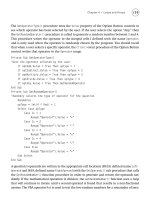
The test t statistic is t
0
= (1.4 − 1.2)/0.083 = 2.35. This is compared with the t distribution with
ν
=
13 degrees of freedom, which is shown in Figure 16.1a. The values t = −2.16 and t = +2.16 that cut off
5% of the area under the curve are shaded in Figure 16.1. Notice that the
α
= 5% is split between 2.5%
on the upper tail plus 2.5% on the lower tail of the distribution. The test value of t
0
= 2.35, located by
the arrow, falls outside this range and therefore is considered to be exceptionally large. We conclude
that it is highly unlikely (less than 5% chance) that such a difference would occur by chance. The
estimate of the true mean concentration, = 1.4, is larger than the standard value,

η
0
= 1.2, by an amount
that cannot be attributed to random experimental error. There must be bias error to explain such a large
difference.
t
0
y
η
0
–
s
y

y
η
0
–
s / n

==
y
y
η
–
t
ν
,a /2
s
y

y
η
+t
ν
,a/2
s
y
<–<–
(y
η
0
– )
yt
ν
,a /2
– s
y

η
yt
ν
,a /2
s
y
+<<
y
y
s
y
y

L1592_Frame_C16 Page 143 Tuesday, December 18, 2001 1:51 PM
© 2002 By CRC Press LLC
In statistical jargon this means “the null hypothesis is rejected.” In engineering terms this means
“there is strong evidence that the measurement method used in these laboratories gives results that are
too high.”
Now we look at the equivalent interpretation using a 95% confidence interval for the difference .
This is constructed using t = 2.16 for
α
/2 = 0.025 and
ν
= 13. The difference has expected value zero
under the null hypothesis, and will vary over the interval mg/L.
The portion of the reference distribution for the difference that falls outside this range is shaded in Figure
16.1b. The difference between the observed and the standard, = 0.2 mg/L, falls beyond the 95%
confidence limits. We conclude that the difference is so large that it is unlikely to occur due to random
variation in the measurement process. “Unlikely” means “a probability of 5% that a difference this large
could occur due to random measurement variation.”
Figure 16.1c is the reference distribution that shows the expected variation of the true mean (
η
) about
the average. It also shows the 95% confidence interval for the mean of the concentration measurements.
The true mean is expected to fall within the range of 1.4 ± 2.16(0.083) = 1.4 ± 0.18. The lower bound
of the 95% confidence interval is 1.22 and the upper bound is 1.58. The standard value of 1.2 mg/L
does not fall within the 95% confidence interval, which leads us to conclude that the true mean of the
measured concentration is higher than 1.2 mg/L.
The shapes of the three reference distributions are identical. The only difference is the scaling of the
horizontal axis, whether we choose to consider the difference in terms of the t statistic, the difference, or
the concentration scale. Many engineers will prefer to make this judgment on the basis of a value scaled
as the measured values are scaled (e.g., as mg/L instead of on the dimensionless scale of the t statistic).
This is done by computing the confidence intervals either for the difference ( ) or for the mean

η
.
The conclusion that the average of the measured concentrations is higher than the known concentration
of 1.2 mg/L could be viewed in two ways. The high average could happen because the measurement
method is biased: only three labs measured less than 1.2 mg/L. Or it could result from the high
concentrations (1.75 mg/L and 1.95 mg/L) measured by two laboratories. To discover which is the case,
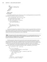
FIGURE 16.1 Three equivalent reference distributions scaled to compare the observed average with the known value on
the basis of the distribution of the (a) t statistic, (b) difference between the observed average and the known level, and (c)
true mean. The distributions were constructed using
η
0
= 1.2 mg/L, = 1.4 mg/L, t
υ
=13,
α
/2=0.025
= 2.16, and = 0.083 mg/L.
3 2 1 0 1 2 3
—
η
s
y
s
y
y
—
η
y
—
η

y

t
0

= 2.35
0
= 0.2
η
0

= 1.2
- 0.3 - 0.2 - 0.1 0 0.1 0.2 0.3

1.1 1.2 1.3 1.4 1.5 1.6 1.7
–
t
True mean, η =
y
– s
y
t
t
statistic,
t
=
True difference,
a
b
c

y S
y
y
η
–
t
13,0.025
s
y
± 2.16(0.083)± 0.18±==
y
η
0
–
y
η
–
L1592_Frame_C16 Page 144 Tuesday, December 18, 2001 1:51 PM
© 2002 By CRC Press LLC
send out more standard specimens and ask the labs to try again. (This may not answer the question.
What often happens when labs get feedback from quality control checks is that they improve their
performance. This is actually the desired result because the objective is to attain uniformly excellent
performance and not to single out poor performers.)
On the other hand, the measurement method might be all right and the true concentration might be
higher than 1.2 mg/L. This experiment does not tell us which interpretation is correct. It is not a simple
matter to make a standard solution for DO; dissolved oxygen can be consumed in a variety of reactions.
Also, its concentration can change upon exposure to air when the specimen bottle is opened in the
laboratory. In contrast, a substance like chloride or zinc will not be lost from the standard specimen, so
the concentration actually delivered to the chemist who makes the measurements is the same concen-
tration in the specimen that was shipped. In the case of oxygen at low levels, such as 1.2 mg/L, it is

not likely that oxygen would be lost from the specimen during handling in the laboratory. If there is a
change, the oxygen concentration is more likely to be increased by dissolution of oxygen from the air.
We cannot rule out this causing the difference between 1.4 mg/L measured and 1.2 mg/L in the original
standard specimens. Nevertheless, the chemists who arranged the test believed they had found a way to
prepare stable test specimens, and they were experienced in preparing standards for interlaboratory tests.
We have no reason to doubt them. More checking of the laboratories seems a reasonable line of action.
Comments
The classical null hypothesis is that “The difference is zero.” No scientist or engineer ever believes this
hypothesis to be strictly true. There will always be a difference, at some decimal point. Why propose a
hypothesis that we believe is not true? The answer is a philosophical one. We cannot prove equality, but
we may collect data that shows a difference so large that it is unlikely to arise from chance. The null
hypothesis therefore is an artifice for letting us conclude, at some stated level of confidence, that there
is a difference. If no difference is evident, we state, “The evidence at hand does not permit me to state
with a high degree of confidence that the measurements and the standard are different.” The null
hypothesis is tested using a t-test.
The alternate, but equivalent, approach to testing the null hypothesis is to compute the interval in which
the difference is expected to fall if the experiment were repeated many, many times. This interval is a
confidence interval. Suppose that the value of a primary standard is 7.0 and the average of several measure-
ments is 7.2, giving a difference of 0.20. Suppose further that the 95% confidence interval shows that the
true difference is between 0.12 to 0.28. This is what we want to know: the true difference is not zero.
A confidence interval is more direct and often less confusing than null hypotheses and significance
tests. In this book we prefer to compute confidence intervals instead of making significance tests.
References
ASTM (1998). Standard Practice for Derivation of Decision Point and Confidence Limit Testing of Mean
Concentrations in Waste Management Decisions, D 6250, Washington, D.C., U.S. Government Printing
Office.
Wilcock, R. J., C. D. Stevenson, and C. A. Roberts (1981).
“An Interlaboratory Study of Dissolved Oxygen
in Water,” Water Res., 15, 321–325.
Exercises

16.1 Boiler Scale. A company advertises that a chemical is 90% effective in cleaning boiler scale
and cites as proof a sample of ten random applications in which an average of 81% of boiler
scale was removed. The government says this is false advertising because 81% does not
equal 90%. The company says the statistical sample is 81% but the true effectiveness may
L1592_Frame_C16 Page 145 Tuesday, December 18, 2001 1:51 PM
© 2002 By CRC Press LLC
easily be 90%. The data, in percentages, are 92, 60, 77, 92, 100, 90, 91, 82, 75, 50. Who is
correct and why?
16.2 Fermentation. Gas produced from a biological fermentation is offered for sale with the
assurance that the average methane content is 72%. A random sample of n = 7 gas specimens
gave methane contents (as %) of 64, 65, 75, 67, 65, 74, and 75. (a) Conduct hypothesis tests
at significance levels of 0.10, 0.05, and 0.01 to determine whether it is fair to claim an average
of 72%. (b) Calculate 90%, 95%, and 99% confidence intervals to evaluate the claim of an
average of 72%.
16.3 TOC Standards. A laboratory quality assurance protocol calls for standard solutions having
50 mg/L TOC to be randomly inserted into the work stream. Analysts are blind to these
standards. Estimate the bias and precision of the 16 most recent observations on such stan-
dards. Is the TOC measurement process in control?
16.4 Discharge Permit. The discharge permit for an industry requires the monthly average COD
concentration to be less than 50 mg/L. The industry wants this to be interpreted as “50 mg/L
falls within the confidence interval of the mean, which will be estimated from 20 observations
per month.” For the following 20 observations, would the industry be in compliance according
to this interpretation of the standard?
50.3 51.2 50.5 50.2 49.9 50.2 50.3 50.5 49.3 50.0 50.4 50.1 51.0 49.8 50.7 50.6
57 60 49 50 51 60 49 53 49 56 64 60 49 52 69 40 44 38 53 66
L1592_Frame_C16 Page 146 Tuesday, December 18, 2001 1:51 PM
© 2002 By CRC Press LLC

17

Paired

t

-Test for Assessing the Average

of Differences

KEY WORDS

confidence intervals, paired

t

-test, interlaboratory tests, null hypothesis

,



t

-test, dissolved
oxygen, pooled variance.

A common question is: “Do two different methods of doing A give different results?” For example, two
methods for making a chemical analysis are compared to see if the new one is equivalent to the older
standard method; algae are grown under different conditions to study a factor that is thought to stimulate
growth; or two waste treatment processes are tested at different levels of stress caused by a toxic input.
In the strict sense, we do not believe that the two analytical methods or the two treatment processes are

identical. There will always be some difference. What we are really asking is: “Can we be highly confident
that the difference is positive or negative?” or “How large might the difference be?”
A key idea is that the

design of the experiment

determines the way we compare the two treatments.
One experimental design is to make a series of tests using treatment A and then to independently make
a series of tests using method B. Because the data on methods A and B are independent of each other,
they are compared by computing the average for each treatment and using an

independent

t

-test

to assess
the difference of the two averages.
A second way of designing the experiment is to pair the samples according to time, technician, batch
of material, or other factors that might contribute to a difference between the two measurements. Now
the test results on methods A and B are produced in pairs that are not independent of each other, so the
analysis is done by averaging the differences for each pair of test results. Then a

paired

t-

test

is used
to assess whether the average of these difference is different from zero. The paired

t

-test is explained
here; the independent

t

-test is explained in Chapter 18.
Two samples are said to be paired when each data point in the first sample is matched and related to
a unique data point in the second sample. Paired experiments are used when it is difficult to control all
factors that might influence the outcome. If these factors cannot be controlled, the experiment is arranged
so they are equally likely to influence both of the paired observations.
Paired experiments could be used, for example, to compare two analytical methods for measuring
influent quality at a wastewater treatment plant. The influent quality will change from moment to moment.
To eliminate variation in influent quality as a factor in the comparative experiment, paired measurements
could be made using both analytical methods on the same specimen of wastewater. The alternative approach
of using method A on wastewater collected on day one and then using method B on wastewater collected
at some later time would be inferior because the difference due to analytical method would be over-
whelmed by day-to-day differences in wastewater quality. This difference between paired same-day tests
is not influenced by day-to-day variation. Paired data are evaluated using the paired

t

-test, which assesses
the average of the differences of the pairs.
To summarize, the test statistic that is used to compare two treatments is as follows: when assessing
the

difference of two averages

, we use the independent

t-

test; when assessing the

average of paired
differences

, we use the paired

t

-test. Which method is used depends on the design of the experiment.
We know which method will be used before the data are collected.
Once the appropriate difference has been computed, it is examined to decide whether we can confidently
declare the difference to be positive, or negative, or whether the difference is so small that we are uncertain

L1592_frame_C17 Page 147 Tuesday, December 18, 2001 1:51 PM
© 2002 By CRC Press LLC

about the direction of the difference. The standard procedure for making such comparisons is to construct
a null hypothesis that is tested statistically using a

t

-test. The classical null hypothesis is: “The difference

between the two methods is zero.” We do not expect two methods to give exactly the same results, so it
may seem strange to investigate a hypothesis that is certainly wrong. The philosophy is the same as in
law where the accused is presumed innocent until proven guilty. We cannot prove a person innocent,
which is why the verdict is worded “not guilty” when the evidence is insufficient to convict. In a statistical
comparison, we cannot prove that two methods are the same, but we can collect evidence that shows
them to be different. The null hypothesis is therefore a philosophical device for letting us avoid saying
that two things are equal. Instead we conclude, at some stated level of confidence, that “there is a diffe-
rence” or that “the evidence does not permit me to confidently state that the two methods are different.”
An alternate, but equivalent, approach to constructing a null hypothesis is to compute the difference and
the interval in which the difference is expected to fall if the experiment were repeated many, many times.
This interval is called the

confidence interval

. For example, we may determine that “A – B

=

0.20 and that
the true difference falls in the interval 0.12 to 0.28, this statement being made at a 95% level of confidence.”
This tells us all that is important. We are highly confident that A gives a result that is, on average, higher
than B. And it tells all this without the sometimes confusing notions of null hypothesis and significance tests.

Case Study: Interlaboratory Study of Dissolved Oxygen

An important procedure in certifying the quality of work done in laboratories is the analysis of standard
specimens that contain known amounts of a substance. These specimens are usually introduced into the
laboratory routine in a way that keeps the analysts blind to the identity of the sample. Often the analyst is
blind to the fact that quality assurance samples are included in the assigned work. In this example, the
analysts were asked to measure the dissolved oxygen (DO) concentration of the same specimen using two

different methods.
Fourteen laboratories were sent a test solution that was prepared to have a low dissolved oxygen
concentration (1.2 mg/L). Each laboratory made the measurements using the Winkler method (a titration)
and the electrode method. The question is whether the two methods predict different DO concentrations.
Table 17.1 shows the data (Wilcock et al., 1981). The observations for each method may be assumed
random and independent as a result of the way the test was designed. The differences plotted in
Figure 17.1 suggest that the Winkler method may give DO measurements that are slightly lower than
the electrode method.

TABLE 17.1

Dissolved Oxygen Data from the Interlaboratory Study

Laboratory 1 2 3 4 567891011121314
Winkler 1.2 1.4 1.4 1.3 1.2 1.3 1.4 2.0 1.9 1.1 1.8 1.0 1.1 1.4
Electrode 1.6 1.4 1.9 2.3 1.7 1.3 2.2 1.4 1.3 1.7 1.9 1.8 1.8 1.8
Diff. (W – E)

−

0.4 0.0

−

0.5

−

1.0

−

0.5 0.0

−

0.8 0.6 0.6

−

0.6

−

0.1

−

0.8

−

0.7

−

0.4

Source:

Wilcock, R. J., C. D. Stevenson, and C. A. Roberts (1981).

Water Res.,

15, 321–325.

FIGURE 17.1

The DO data and the differences of the paired values.
2
0
-2
1 5 10 14
Laboratory
Difference (W – E)

L1592_frame_C17 Page 148 Tuesday, December 18, 2001 1:51 PM
© 2002 By CRC Press LLC

Theory: The Paired

t

-Test Analysis

Define

δ

as the true mean of differences between random variables

y

1

and

y

2

that were observed as
matched pairs under identical experimental conditions.

δ

will be zero if the means of the populations
from which

y

1

and

y

2

are drawn are equal. The estimate of

δ

is the average of differences between

n

paired observations:
Because of measurement error, the value of is not likely to be zero, although it will tend toward zero
if

δ

is zero.
The sample variance of the differences is:
The standard error of the average difference is:
This is used to establish the 1 –

α

confidence limits for

δ

, which are . The correctness of
this confidence interval depends on the data being independent and coming from distributions that are
approximately normal with the same variance.

Case Study Solution

The differences were calculated by subtracting the electrode measurements from the Winkler measure-
ments. The average of the paired differences is:
and the variance of the paired differences is:
giving

s

d



=

0.494 mg/L. The standard error of the average of the paired differences is:
The (1 –

α

)100% confidence interval is computed using the

t

distribution with

ν



=

13 degrees of freedom
at the

α

/

2 probability point. For (1

−



α

)

=

0.95,

t

13,0.025



=

2.160, and the 95% confidence interval of the

true difference

δ

is:
d
∑d
i
n

1
n

y
1,i
y
2,i
–()
∑
==
d
s
d
2
∑ d
i
d–()
2
n 1–

=
d
s
d
s
d
n

=
ds
d
t
n−1,
α
/2
±
d
0.4–()00.5–()1.0–()
…
0.4–()++ + + +
14

0.329 mg/L–==
s
d
2
0.4– 0.329–()–[]
2
0 0.329–()–[]
2

…
0.4– 0.329–()–[]
2
+++
14 1–

0.244 mg/L()
2
==
s
d
0.494
14

0.132 mg/L==
ds
d
t
13,0.025

δ
ds+
d
t
13,0.025
<<–

L1592_frame_C17 Page 149 Tuesday, December 18, 2001 1:51 PM
© 2002 By CRC Press LLC

For the particular values of this example:
–0.326 – 0.132(2.160) <

δ

< –0.326

+

0.132(2.160)
–0.61 mg/L <

δ

< –0.04 mg/L
We are highly confident that the difference between the two methods is not zero because the confidence
interval does not include the difference of zero. The methods give different results and, furthermore, the
electrode method has given higher readings than the Winkler method.
If the confidence interval had included zero, the interpretation would be that we cannot say with a
high degree of confidence that the methods are different. We should be reluctant to report that the methods
are the same or that the difference between the methods is zero because what we know about chemical
measurements makes it unlikely that these statements are strictly correct. We may decide that the difference
is small enough to have no practical importance. Or the range of the confidence interval might be large
enough that the difference, if real, would be important, in which case additional tests should be done to
resolve the matter.
An alternate but equivalent evaluation of the results is to test the null hypothesis that

the difference
between the two averages is zero

. The way of stating the conclusion when the 95% confidence interval
does not include zero is to say that “the difference was significant at the 95% confidence level.”
Significant, in this context, has a purely statistical meaning. It conveys nothing about how interesting
or important the difference is to an engineer or chemist. Rather than reporting that the difference was
significant (or not), communicate the conclusion more simply and directly by giving the confidence
interval. Some reasons for preferring to look at the confidence interval instead of doing a significance
test are given at the end of this chapter.
Why Pairing Eliminates Uncontrolled Disturbances
Paired experiments are used when it is difficult to control all the factors that might influence the outcome.
A paired experimental design ensures that the uncontrolled factors contribute equally to both of the
paired observations. The difference between the paired values is unaffected by the uncontrolled distur-
bances, whereas the differences of unpaired tests would reflect the additional component of experimental
error. The following example shows how a large seasonal effect can be blocked out by the paired design.
Block out means that the effect of seasonal and day-to-day variations are removed from the comparison.
Blocking works like this. Suppose we wish to test for differences in two specimens, A and B, that are
to be collected on Monday, Wednesday, and Friday (M, W, F). It happens, perhaps because of differences
in production rate, that Wednesday is always two (2) units higher than Monday, and Friday is always
three (3) units higher than Monday. The data are:
This day-to-day variation is blocked out if the analysis is done on (A – B)
M
, (A – B)
W
, and (A – B)
F
instead of the alternate (A
M
+ A
W
+ A
F

)/3 = and (B
M
+ B
W
+ B
F
)/3 = . The difference between A
and B is two (2) units. This is true whether we calculate the average of the differences [(2 + 2 + 2)/3 = 2]
or the difference of the averages [6.67 – 4.67 = 2]. The variance of the differences is zero, so it is clear
that the difference between A and B is 2.0.
Method
Day A B Difference
M532
W752
F 8 6 2
Averages 6.67 4.67 2
Variances 2.3 2.3 0
A B
L1592_frame_C17 Page 150 Tuesday, December 18, 2001 1:51 PM
© 2002 By CRC Press LLC
A t-test on the difference of the averages would conclude that A and B are not different. The reason
is that the variance of the averages over M, W, and F is inflated by the day-to-day variation. This day-
to-day variation overwhelms the analysis; pairing removes the problem.
The experimenter who does not think of pairing (blocking) the experiment works at a tremendous
handicap and will make many wrong decisions. Imagine that the collecting for A was done on M, W,
F, of one week and collection for B was done in another week. Now the paired analysis cannot be done
and the difference will not be detected. This is why we speak of a paired design as well as of a paired
t-test analysis. The crucial step is making the correct design. Pairing is always recommended.
Case Study to Emphasize the Benefits of a Paired Design
A once-through cooling system at a power plant is suspected of reducing the population of certain aquatic

organisms. The copepod population density (organisms per cubic meter) were measured at the inlet and
outlet of the cooling system on 17 different days (Simpson and Dudaitis, 1981). On each sampling day,
water specimens were collected within a short time interval, first at the inlet and then at the outlet. The
sampling plan represents a thoughtful effort to block out the effect of day-to-day and month-to-month
variations in population counts. It pairs the inlet and outlet measurements. Of course, it is impossible
to sample the same parcel of water at the inlet and outlet (i.e., the pairing is not exact), but any variation
caused by this will be reflected as a component of the random measurement error.
The data are plotted in Figure 17.2. The plot gives the impression that the cooling system may not
affect the copepods. The outlet counts are higher than inlets counts on 10 of the 17 days. There are
some big differences, but these are on days when the count was very high and we expect that the
measurement error in counting will be proportional to the population. (If you count 10 pennies you
will get the right answer, but if you count 1000, you are certain to have some error; the more pennies
the more counting error.) Before doing the calculations, consider once more why the paired comparison
should be done.
Specimens 1 through 6 were taken in November 1977, specimens 7 through 12 in February 1978, and
specimens 13 through 17 in August 1978. A large seasonal variation is apparent. If we were to compute
the variances of the inlet and outlet counts, it would be huge and it would consist largely of variation
due to seasonal differences. Because we are not trying to evaluate seasonal differences, this would be a
poor way to analyze the data. The paired comparison operates on the differences of the daily inlet and
outlet counts, and these differences do not reflect the seasonal variation (except, as we shall see in a
moment, to the extent that the differences are proportional to the population density).
FIGURE 17.2 Copepod population density (organisms/m
3
).
Sample
Outlet
Inlet
Copepod Density
0
20000

40000
60000
80000
1 2 3 4 5 6 7 8 9 10 11 12 13 14 15 16 17
L1592_frame_C17 Page 151 Tuesday, December 18, 2001 1:51 PM
© 2002 By CRC Press LLC
It is tempting to tell ourselves that “I would not be foolish enough not to do a paired comparison on
data such as these.” Of course we would not when the variation due to the nuisance factor (season) is
both huge and obvious. But almost every experiment is at risk of being influenced by one or more nuisance
factors, which may be known or unknown to the experimenter. Even the most careful experimental tech-
nique cannot guarantee that these will not alter the outcome. The paired experimental design will prevent
this and it is recommended whenever the experiment can be so arranged.
Biological counts usually need to be transformed to make the variance uniform over the observed range
of values. The paired analysis will be done on the differences between inlet and outlet, so it is the variance
of these differences that should be examined. The differences are plotted in Figure 17.3. Clearly, the differ-
ences are larger when the counts are larger, which means that the variance is not constant over the range
of population counts observed. Constant variance is one condition of the t-test because we want each
observation to contribute in equal weight to the analysis. Any statistics computed from these data would
be dominated by the large differences of the high population counts and it would be misleading to construct
a confidence interval or test a null hypothesis using the data in their original form.
A transformation is needed to make the variance constant over the ten-fold range of the counts in the
sample. A square-root transformation is often used on biological counts (Sokal and Rohlf, 1969), but
for these data a log transformation seemed to be better. The bottom section of Figure 17.3 shows that
the differences of the log-transformed data are reasonably uniform over the range of the transformed
values.
Table 17.2 shows the data, the transformed data [z = ln(y)], and the paired differences. The average
difference of ln(in) − ln(out) is = −0.051. The variance of the differences is s
2
= ∑(d
i

− )
2
/
16 = 0.014 and the standard error of average difference = 0.029.
The 95% confidence interval is constructed using t
16,0.025
= 2.12. It can be stated with 95% confidence
that the true difference falls in the region:
−0.051 − 2.12(0.029) <
δ
ln
< −0.051 + 2.12(0.029)
−0.112 <
δ
ln
< 0.010
This confidence interval includes zero so we can state with a high degree of confidence that outlet counts
are not less than inlet counts.
FIGURE 17.3 The difference in copepod inlet and outlet population density is larger when the population is large, indicating
nonconstant variance at different population levels.
-15000
-10000
-5000
0
5000
-0.3
-0.2
-0.1
0.0
0.1

0.2
0.3
800006000040000200000
12111098
Inlet Copepod Density
In (Inlet Copepod Density)
Density Difference
(Inlet - Outlet)
Density Difference
In (In) - (Out)
d ∑d
in
/17= d
s
d
s / 17=
d
ln
s
d
t
16,0.025
δ
ln
d
ln
s
d
t
16,0.025

+<<–
L1592_frame_C17 Page 152 Tuesday, December 18, 2001 1:51 PM
© 2002 By CRC Press LLC
Comments
The paired t-test examines the average of the differences between paired observations. This is not
equivalent to comparing the difference of the average of two samples that are not paired. Pairing blocks
out the variation due to uncontrolled or unknown experimental factors. As a result, the paired experi-
mental design should be able to detect a smaller difference than an unpaired design. We do not have
free choice of which t-test to use for a particular set of data. The appropriate test is determined by the
experimental design.
We never really believe the null hypothesis. It is too much to expect that the difference between any
two methods is truly zero. Tukey (1991) states this bluntly:
Statisticians classically asked the wrong question — and were willing to answer with a lie …
They asked “Are the effects of A and B different?” and they were willing to answer “no.”
All we know about the world teaches us that A and B are always different — in some decimal
place. Thus asking “Are the effects different?” is foolish.
What we should be answering first is “Can we be confident about the direction from method
A to method B? Is it up, down, or uncertain?”
If uncertain whether the direction is up or down, it is better to answer “we are uncertain about the
direction” than to say “we reject the null hypothesis.” If the answer was “direction certain,” the follow-
up question is how big the difference might be. This question is answered by computing confidence
intervals.
Most engineers and scientists will like Tukey’s view of this problem. Instead of accepting or rejecting
a null hypothesis, compute and interpret the confidence interval of the difference. We want to know
the confidence interval anyway, so this saves work while relieving us of having to remember exactly
what it means to “fail to reject the null hypothesis.” And it lets us avoid using the words statistically
significant.
TABLE 17.2
Outline of Computations for a Paired t-Test on the Copepod Data after a Logarithmic
Transformation

Original Counts (no./m
3
) Transformed Data, z ==
==
ln( y)
Sample y
in
y
out
d ==
==
y
in
−−
−−
y
out
z
in
z
out
d
ln
==
==
z
in
−−
−−
z

out
1 44909 47069 −2160 10.712 10.759 −0.047
2 42858 50301 −7443 10.666 10.826 −0.160
3 35976 40431 −4455 10.491 10.607 −0.117
4 20048 24887 −4839 9.906 10.122 -0.216
5 28273 28385 −112 10.250 10.254 −0.004
6 27261 26122 1139 10.213 10.171 0.043
7 66149 72039 −5890 11.100 11.185 −0.085
8 70190 70039 151 11.159 11.157 0.002
9 53611 63228 −9617 10.890 11.055 −0.165
10 49978 60585 −10607 10.819 11.012 −0.192
11 39186 47455 −8269 10.576 10.768 −0.191
12 41074 43584 −2510 10.623 10.682 −0.059
13 8424 6640 1784 9.039 8.801 0.238
14 8995 8244 751 9.104 9.017 0.087
15 8436 8204 232 9.040 9.012 0.028
16 9195 9579 −384 9.126 9.167 −0.041
17 8729 8547 182 9.074 9.053 0.021
Average 33135 36196 –3062 10.164 10.215 −0.051
Std. deviation 20476 23013 4059 0.785 0.861 0.119
Std. error 4967 5582 984 0.190 0.209 0.029
L1592_frame_C17 Page 153 Tuesday, December 18, 2001 1:51 PM
© 2002 By CRC Press LLC
To further emphasize this, Hooke (1963) identified these inadequacies of significance tests.
1. The test is qualitative rather than quantitative. In dealing with quantitative variables, it is
often wasteful to point an entire experiment toward determining the existence of an effect
when the effect could also be measured at no extra cost. A confidence statement, when it can
be made, contains all the information that a significance statement does, and more
.
2. The word “significance” often creates misunderstandings, owing to the common habit of

omitting the modifier “statistical.” Statistical significance merely indicates that evidence of
an effect is present, but provides no evidence in deciding whether the effect is large enough
to be important. In a given experiment, statistical significance is neither necessary nor sufficient
for scientific or practical importance. (emphasis added)
3. Since statistical significance means only that an effect can be seen in spite of the experimental
error (a signal is heard above the noise), it is clear that the outcome of an experiment depends
very strongly on the sample size. Large samples tend to produce significant results, while
small samples fail to do so.
Now, having declared that we prefer not to state results as being significant or nonsignificant, we pass
on two tips from Chatfield (1983) that are well worth remembering:
1. A nonsignificant difference is not necessarily the same thing as no difference.
2. A significant difference is not necessarily the same thing as an interesting difference.
References
Chatfield, C. (1983). Statistics for Technology, 3rd ed., London, Chapman & Hall.
Hooke, R. (1963). Introduction to Scientific Inference, San Francisco, CA, Holden-Day.
Simpson, R. D. and A. Dudaitis (1981). “Changes in the Density of Zooplankton Passing Through the Cooling
System of a Power-Generating Plant,” Water Res., 15, 133–138.
Sokal, R. R. and F. J. Rohlf (1969). Biometry: The Principles and Practice of Statistics in Biological Research,
New York, W. H. Freeman and Co.
Tukey, J. W. (1991). “The Philosophy of Multiple Comparisons,” Stat. Sci., 6(6), 100–116.
Wilcock, R. J., C. D. Stevenson, and C. A. Roberts (1981). “An Interlaboratory Study of Dissolved Oxygen
in Water,” Water Res., 15, 321–325.
Exercises
17.1 Antimony. Antimony in fish was measured in three paired samples by an official standard
method and a new method. Do the two methods differ significantly?
17.2 Nitrite Measurement. The following data were obtained from paired measurements of nitrite
in water and wastewater by direct ion-selective electrode (ISE) and a colorimetric method.
Are the two methods giving consistent results?
Sample No. 1 2 3
New method 2.964 3.030 2.994

Standard method 2.913 3.000 3.024
L1592_frame_C17 Page 154 Tuesday, December 18, 2001 1:51 PM
© 2002 By CRC Press LLC
17.3 BOD Tests. The data below are paired comparisons of BOD tests done in standard 300-mL
bottles and experimental 60-mL bottles. Estimate the difference and the confidence interval
of the difference between the results for the two bottle sizes.
17.4 Leachate Tests. Paired leaching tests on a solid waste material were conducted for contact
times of 30 and 75 minutes. Based on the following data, is the same amount of tin leached
from the material at the two leaching times?
17.5 Stream Monitoring. An industry voluntarily monitors a stream to determine whether its goal
of raising the level of pollution by 4 mg/L or less is met. The observations below for September
and April were made every fourth working day. Is the industry’s standard being met?
Method Nitrite Measurements
ISE 0.32 0.36 0.24 0.11 0.11 0.44 2.79 2.99 3.47
Colorimetric 0.36 0.37 0.21 0.09 0.11 0.42 2.77 2.91 3.52
300 mL 7.2 4.5 4.1 4.1 5.6 7.1 7.3 7.7 32 29 22 23 27
60 mL 4.8 4.0 4.7 3.7 6.3 8.0 8.5 4.4 30 28 19 26 28
Source: McCutcheon, S. C., J. Env. Engr. ASCE, 110, 697–701.
Leaching Time
(min)
Tin Leached
(mg/ kg)
30 51 60 48 52 46 58 56 51
75 57 57 55 56 56 55 56 55
September April
Upstream Downstream Upstream Downstream
7.5 12.5 4.6 15.9
8.2 12.5 8.5 25.9
8.3 12.5 9.8 15.9
8.2 12.2 9.0 13.1

7.6 11.8 5.2 10.2
8.9 11.9 7.3 11.0
7.8 11.8 5.8 9.9
8.3 12.6 10.4 18.1
8.5 12.7 12.1 18.3
8.1 12.3 8.6 14.1
L1592_frame_C17 Page 155 Tuesday, December 18, 2001 1:51 PM
© 2002 By CRC Press LLC

18

Independent

t

-Test for Assessing the Difference

of Two Averages

KEY WORDS

confidence interval, independent

t

-test, mercury.

Two methods, treatments, or conditions are to be compared. Chapter 17 dealt with the experimental design
that produces measurements from two treatments that were paired. Sometimes it is not possible to pair the
tests, and then the averages of the two treatments must be compared using the

independent

t

-test

.

Case Study: Mercury in Domestic Wastewater

Extremely low limits now exist for mercury in wastewater effluent limits. It is often thought that whenever
the concentration of heavy metals is too high, the problem can be corrected by forcing industries to stop
discharging the offending substance. It is possible, however, for target effluent concentrations to be so
low that they might be exceeded by the concentration in domestic sewage. Specimens of drinking water
were collected from two residential neighborhoods, one served by the city water supply and the other
served by private wells. The observed mercury concentrations are listed in Table 18.1. For future studies
on mercury concentrations in residential areas, it would be convenient to be able to sample in either
neighborhood without having to worry about the water supply affecting the outcome. Is there any
difference in the mercury content of the two residential areas?
The sample collection cannot be paired. Even if water specimens were collected on the same day,
there will be differences in storage time, distribution time, water use patterns, and other factors. Therefore,
the data analysis will be done using the independent

t

-test.

t

-Test to Compare the Averages of Two Samples

Two independently distributed random variables

y

1

and

y

2

have, respectively, mean values

η

1

and

η

2

and
variances and . The usual statement of the problem is in terms of testing the null hypothesis that
the difference in the means is zero:

η

1



−



η

2



=

0, but we prefer viewing the problem in terms of the
confidence interval of the difference.
The expected value of the difference between the averages of the two treatments is:
If the data are from random samples, the variances of the averages and are:
where

n

1

and

n

2

are the sample sizes. The variance of the difference is:

σ
1
2
σ
2
2
Ey
1
y
2
–()
η
1
η
2
–=
y
1
y
2
Vy
1
()
σ

1
2
/n
1
and Vy
2
()
σ
2
2
/n
2
==
Vy
1
y
2
–()
σ
1
2
n
1

σ
2
2
n
2

+=

L1592_frame_C18.fm Page 157 Tuesday, December 18, 2001 1:52 PM
© 2002 By CRC Press LLC

Usually the variances and are unknown and must be estimated from the sample data by computing:
These can be pooled if they are of equal magnitude. Assuming this to be true, the pooled estimate of
the variance is:
This is the weighted average of the variances, where the weights are the degrees of freedom of each
variance. The number of observations used to compute each average and variance need not be equal.
The estimated variance of the difference is:
and the standard error is the square root:
Student’s

t

distribution is used to compute the level confidence interval. To construct the (1

−



α

)100%
percent confidence interval use the

t

statistic for

α

/

2 and

ν



=



n

1



+



n

2

−

2 degrees of freedom.
The correctness of this confidence interval depends on the data being independent and coming from
distributions that are approximately normal with the same variance. If the variances are very different
in magnitude, they cannot be pooled unless uniform variance can be achieved by means of a transfor-
mation. This procedure is robust to moderate nonnormality because the central limit effect will tend to
make the distributions of the averages and their difference normal even when the parent distributions of

y

1

and

y

2

are not normal.

Case Solution: Mercury Data

Water specimens collected from a residential area that is served by the city water supply are indicated
by subscript

c

;

p

indicates specimens taken from a residential area that is served by private wells. The
averages, variances, standard deviations, and standard errors are:

TABLE 18.1

Mercury Concentrations in Wastewater Originating in an Area Served by the City Water Supply (

c

) and an

Area Served by Private Wells (

p

)

Source Mercury Concentrations (

µµ
µµ

g/L)

City (

n

c



=

13) 0.34 0.18 0.13 0.09 0.16 0.09 0.16 0.10 0.14 0.26 0.06 0.26 0.07
Private (

n

p



=

10) 0.26 0.06 0.16 0.19 0.32 0.16 0.08 0.05 0.10 0.13

Data provided by Greg Zelinka, Madison Metropolitan Sewerage District.

City (

n

c

=

13)

=

0.157

µ

g

/

L

=

0.0071

=

0.084

=

0.023
Private (

n

p



=

10)

=

0.151

µ

g

/

L

=

0.0076

=

0.087

=

0.028
σ
1
2
σ
2
2
s
1
2
∑ y
1i
y
1
–()
2
n
1
1–

and s
2
2
∑ y
2i
y
2
–()
2

n
2
1–

==
s
pool
2
n
1
1–()s
1
2
n
2
1–()s
2
2
+
n
1
n
2
2–+

=
Vy
1
y
2

–()
s
pool
2
n
1

s
pool
2
n
2

+ s
pool
2
1
n
1

1
n
2

+


==
s
y

1
−y
2
s
pool
2
n
1

s
pool
2
n
2

+ s
pool
1
n
1

1
n
2

+==
y
c
s
c

2
s
c
s
y
c
y
p
s
p
2
s
p
s
y
p
L1592_frame_C18.fm Page 158 Tuesday, December 18, 2001 1:52 PM
© 2002 By CRC Press LLC
The difference in the averages of the measurements is = 0.157 − 0.151 = 0.006
µ
g/L. The
variances and of the city and private samples are nearly equal, so they can be pooled by weighting
in proportion to their degrees of freedom:
The estimated variance of the difference between averages is:
and the standard error of = 0.006
µ
g/L is = = 0.036
µ
g/L.
The variance of the difference is estimated with

ν
= 12 + 9 = 21 degrees of freedom. The 95%
confidence interval is calculated using
α
/2 = 0.025 and t
21,0.025
= 2.080:
It can be stated with 95% confidence that the true difference between the city and private water supplies
falls in the interval of −0.069
µ
g/L and 0.081
µ
g/L. This confidence interval includes zero so there is
no persuasive evidence in these data that the mercury contents are different in the two residential areas.
Future sampling can be done in either area without worrying that the water supply will affect the outcome.
Comments
The case study example showed that one could be highly confident that there is no statistical difference
between the average mercury concentrations in the two residential neighborhoods. In planning future
sampling, therefore, one might proceed as though the neighborhoods are identical, although we under-
stand that this cannot be strictly true.
Sometimes a difference is statistically significant but small enough that, in practical terms, we do not
care. It is statistically significant, but unimportant. Suppose that the mercury concentrations in the city and
private waters had been 0.15 mg/L and 0.17 mg/L (not
µ
g/L) and that the difference of 0.02 mg/L was
statistically significant. We would be concerned about the dangerously high mercury levels in both neigh-
borhoods. The difference of 0.02 mg/L and its statistical significance would be unimportant. This reminds
us that significance in the statistical sense and important in the practical sense are two different concepts.
In this chapter the test statistic used to compare two treatments was the difference of two averages
and the comparison was made using an independent t-test. Independent, in this context, means that all

sources of uncontrollable random variation will equally affect each treatment. For example, specimens
tested on different days will reflect variation due to any daily difference in materials or procedures in
addition to the random variations that always exist in the measurement process. In contrast, Chapter 17
explains how a paired t-test will block out some possible sources of variation. Randomization is also
effective for producing independent observations.
Exercises
18.1 Biosolids. Biosolids from an industrial wastewater treatment plant were applied to 10 plots
that were randomly selected from a total of 20 test plots of farmland. Corn was grown on
the treated (T) and untreated (UT) plots, with the following yields (bushels/acre).
Calculate a 95% confidence limit for the difference in means.
UT 126 122 90 135 95 180 68 99 122 113
T 144 122 135 122 77 149 122 117 131 149
y
c
y
p
–
s
c
2
s
p
2
s
pool
2
12 0.0071()9 0.0076()+
12 9+

0.00734

µ
g/L()
2
==
Vy
c
y
p
–()s
y
c
2
s
y
p
2
+ s
pool
2
1
n
c

1
n
p

+



0.00734
1
13

1
10

+


0.0013
µ
g/L()
2
== = =
y
c
y
p
– s
y
c
−y
p
0.0013
y
c
y
p
–()t

21,0.025
s
y
c
−y
p
± 0.006 2.080 0.036()± 0.006 0.075
µ
g/L±==
L1592_frame_C18.fm Page 159 Tuesday, December 18, 2001 1:52 PM
© 2002 By CRC Press LLC
18.2 Lead Measurements. Below are measurements of lead in solutions that are identical except
for the amount of lead that has been added. Fourteen specimens had an addition of 1.25
µ
g/L
and 14 had an addition of 2.5
µ
g/L. Is the difference in the measured values consistent with
the known difference of 1.25
µ
g/L?
18.3 Bacterial Densities. The data below are the natural logarithms of bacterial counts as measured
by two analysts on identical aliquots of river water. Are the analysts getting the same result?
18.4 Highway TPH Contamination. Use a t-test analysis of the data in Exercise 3.6 to compare
the TPH concentrations on the eastbound and westbound lanes of the highway.
18.5 Water Quality. A small lake is fed by streams from a watershed that has a high density of
commercial land use, and a watershed that is mainly residential. The historical data below
were collected at random intervals over a period of four years. Are the chloride and alkalinity
of the two streams different?
Addition ==

==
1.25
µµ
µµ
g//
//
L 1.1 2.0 1.3 1.0 1.1 0.8 0.8 0.9 0.8 1.6 1.1 1.2 1.3 1.2
Addition ==
==
2.5
µµ
µµ
g//
//
L 2.8 3.5 2.3 2.7 2.3 3.1 2.5 2.5 2.5 2.7 2.5 2.5 2.6 2.7
Analyst A 1.60 1.74 1.72 1.85 1.76 1.72 1.78
Analyst B 1.72 1.75 1.55 1.67 2.05 1.51 1.70
‘
Commercial Land Use Residential Land Use
Chloride
(mg/L)
Alkalinity
(mg /L)
Chloride
(mg/L)
Alkalinity
(mg/L)
‘
140 49 120 40
135 45 114 38

130 28 142 38
132 40 100 45
135 38 100 43
145 43 92 51
118 36 122 33
157 48 97 45
145 51
130 55
‘
L1592_frame_C18.fm Page 160 Tuesday, December 18, 2001 1:52 PM
© 2002 By CRC Press LLC

19

Assessing the Difference of Proportions

KEY WORDS

bioassay, binomial distribution, binomial model, censored data, effluent testing, normal
distribution, normal approximation, percentages, proportions, ratio, toxicity

,



t

-test.

Ratios and proportions arise in biological, epidemiological, and public health studies. We may want to

study the proportion of people infected at a given dose of virus, the proportion of rats showing tumors
after exposure to a carcinogen, the incidence rate of leukemia near a contaminated well, or the proportion
of fish affected in bioassay tests on effluents. Engineers would study such problems only with help from
specialists, but they still need to understand the issues and some of the relevant statistical methods.
A situation where engineers will use ratios and proportions is when samples have been censored by
a limit of detection. A data set on an up-gradient groundwater monitoring well has 90% of all observations
censored and a down-gradient well has only 75% censored. Does this difference indicate that contami-
nation has occurred in the groundwater flowing between the two wells?

Case Study

Biological assays are a means of determining the toxicity of an effluent. There are many ways such tests
might be organized: species of test organism, number of test organisms, how many dilutions of effluent
to test, specification of response, physical conditions, etc. Most of these are biological issues. Here we
consider some statistical issues in a simple bioassay.
Organisms will be put into (1) an aquarium containing effluent or (2) a control aquarium containing
clean water. Equal numbers of organisms are assigned randomly to the control and effluent groups. The
experimental response is a binary measure: presence or absence of some characteristic. In an acute
bioassay, the binary characteristic is survival or death of the organism. In a chronic bioassay, the organisms
are exposed to nonlethal conditions and the measured response might be loss of equilibrium, breathing
rate, loss of reproductive capacity, rate of weight gain, formation of neoplasms, etc.
In our example, 80 organisms (

n

1



=

n

2



=

80) were exposed to each treatment condition (control and
effluent) and toxicity was measured in terms of survival. The data shown in Table 19.1 were observed.
Are the survival proportions in the two groups so different that we can state with a high degree of
confidence that the two treatments truly differ in toxicity?

The Binomial Model

The data from a binomial process consist of two discrete outcomes (binary). A test organism is either
dead or alive after a given period of time. An effluent is either in compliance or it is not. In a given
year, a river floods or it does not flood. The binomial probability distribution gives the probability of
observing an event

x

times in a set of

n

trials (experiment). If the event is observed, the trial is said to

be successful. Success in this statistical sense does not mean that the outcome is desirable. A success
may be the death of an organism, failure of a machine, or violation of a regulation. It means success in

L1592_frame_C19.fm Page 161 Tuesday, December 18, 2001 1:53 PM
© 2002 By CRC Press LLC

observing the behavior of interest. The true probability of the event of interest occurring in a given trial
is

p

, and 1

−



p

is the probability of the event not occurring. In most environmental problems, the desired
outcome is for the event to occur infrequently, which means that we are interested in cases where both

x

and

p

are small.
The

binomial probability

that

x

will occur for given values of

n

and

p

is:
The terms with the factorials indicates the number of ways that

x

successes can occur in a sample of
size

n

. These terms are known as the

binomial coefficients

. The probability of a success in a single trial

is

p

(the corresponding probability of failure in a single trial is (1

−



p

). The expected number of
occurrences in

n

trials is the mean of

x

, which is

µ

x



=

np

. The variance is

=



np

(1

−



p

). This will be
correct when

p

is constant and outcomes are independent from trial to trial.
The probability of

r

or fewer success in

n

independent trials for a probability of success

p

in a single
trial is given by the cumulative binomial distribution:

Table 19.2, calculated from this equation, gives the cumulative probability of

x

successes in

n



=

20 trials
for several values of

p

. Table 19.3, which gives the probability of

exactly



x

occurrences for the same

TABLE 19.1

Data from a Bioassay on Wastewater Treatment Plant Effluent

Number

%
Group Surviving Not Surviving Totals Surviving Not Surviving

Control 72 8 80 90 10
Effluent 64 16 80 80 20
Totals 136 24 160 Avg.

=

85 15

TABLE 19.2

Cumulative Binomial Probability for

x

Successes in 20 Trials, where

p



is the True Random Probability of Success in a Single Trial

xp



==
==

0.05 0.10 0.15 0.20 0.25 0.50

0 0.36 0.12 0.04 0.01 0.00 0.00
1 0.74 0.39 0.18 0.07 0.02 0.00
2 0.92 0.68 0.40 0.21 0.09 0.00
3 0.98 0.87 0.65 0.41 0.23 0.00
4 1.00 0.96 0.83 0.63 0.41 0.01
5 1.00 0.99 0.93 0.80 0.62 0.02
6 1.00 0.98 0.91 0.79 0.06
7 1.00 0.99 0.97 0.90 0.13
8 1.00 0.99 0.96 0.25
9 1.00 1.00 0.99 0.41
10 1.00 1.00 0.59

11 1.00 0.75
12 0.87
13 0.94
14 0.98
15 0.99
16 1.00
f
x: n, p()
n!
x! nx–()!

p
x
1 p–()
n−x
x 0, 1, 2, …, n==
σ
x
2
Pr xr≤()Fr: n, p()
n!
x! nx–()!

p
x
1 p–()
n−x
0
r
∑

==

L1592_frame_C19.fm Page 162 Tuesday, December 18, 2001 1:53 PM