Statistics for Environmental Engineers Second Edition phần 6 pptx

© 2002 By CRC Press LLC

The data in Table 26.1 were collected at a municipal incinerator by the Danish Environmental Agency
(Pallesen, 1987). Two different kinds of samplers were used to take simultaneous samples during four
3.5-hour sampling periods, spread over a three-day period. Operating load, temperature, pressure, etc.
were variable. Each sample was analyzed for five dioxin groups (TetraCDD, PentaCDD, HexaCDD,
HeptaCDD, and OctoCDD) and five furan groups (TetraCDF, PentaCDF, HexaCDF, HeptaCDF, and
OctoCDF). The species within each group are chlorinated to different degrees (4, 5, 6, 7, and 8 chlorine
atoms per molecule). All analyses were done in one laboratory.
There are four factors being evaluated in this experiment: two kinds of samplers (S), four sampling
periods (P), two dioxin and furan groups (DF), five levels of chlorination within each group (CL). This
gives a total of

n



=

2

×

4

×

2

×

5

=

80 measurements. The data set is completely balanced; all conditions
were measured once with no repeats. If there are any missing values in an experiment of this kind, or if
some conditions are measured more often than others, the analysis becomes more difficult (Milliken and
Johnson, 1992).
When the experiment was designed, the two samplers were expected to perform similarly but that
variation over sampling periods would be large. It was also expected that the levels of dioxins and furans,
and the amounts of each chlorinated species, would be different. There was no prior expectation regarding
interactions. A four-factor analysis of variance (ANOVA) was done to assess the importance of each
factor and their interactions.

Method: Analysis of Variance

Analysis of variance addresses the problem of identifying which factors contribute significant amounts
of variance to measurements. The general idea is to partition the total variation in the data and assign
portions to each of the four factors studied in the experiment and to their interactions.
Total variance is measured by the total residual sum of squares:
where the residuals are the deviations of each observation from the grand mean

TABLE 26.1

Dioxin and Furan Data from a Designed Factorial Experiment

Sample Period

1

2

3

4
Sampler A B ABABAB

Dioxins
Sum TetraCDD 0.4 1.9 0.5 1.7 0.3 0.7 1.0 2.0
Sum PentaCDD 1.8 28 3.0 7.3 2.7 5.5 7.0 11
Sum HexaCDD 2.5 24 2.6 7.3 3.8 5.1 4.7 6.0
Sum HeptaCDD 17 155 16 62 29 45 30 40
OctoCDD 7.4 55 7.3 28 14 21 12 17
Furans
Sum TetraCDF 4.9 26 7.8 18 5.8 9.0 13 13
Sum PentaCDF 4.2 31 11 22 7.0 12 17 24
Sum HexaCDF 3.5 31 11 28 8.0 14 18 19
Sum HeptaCDF 9.1 103 32 80 32 41 47 62
OctoCDF 3.8 19 6.4 18 6.6 7.0 6.7 6.7

Note:

Values shown are concentrations in ng

/

m

3

normal dry gas at actual CO

2

percentage.
Total SS y
obs
y–()
2
all obs
n
∑
=
y
1
n

y
i
all obs
n
∑
=

L1592_frame_C26.fm Page 234 Tuesday, December 18, 2001 2:46 PM
© 2002 By CRC Press LLC

of the

n

=

80 observations. This is also called the total adjusted sum of squares (corrected for the mean).
Each of the

n

observations provides one degree of freedom. One of them is consumed in computing the
grand average, leaving

n



−

1 degrees of freedom available to assign to each of the factors that contribute
variability. The Total SS and its

n



−

1 degrees of freedom are separated into contributions from the factors
controlled in the experimental design. For the dioxin/furan emissions experiment, these sums of squares

(SS) are:
Another approach is to specify a general model to describe the data. It might be simple, such as:
where the Greek letters indicate the true response due to the four factors and

e

i

is the random residual
error of the

i

th observation. The residual errors are assumed to be independent and normally distributed
with mean zero and constant variance

σ

2

(Rao, 1965; Box et al., 1978).
The assumptions of independence, normality, and constant variance are not equally important to the
ANOVA. Scheffe (1959) states, “In practice, the statistical inferences based on the above model are not
seriously invalidated by violation of the normality assumption, nor,…by violation of the assumption of
equality of cell variances. However, there is no such comforting consideration concerning violation of the
assumption of statistical independence, except for experiments in which randomization has been incor-
porated into the experimental procedure.”
If measurements had been replicated, it would be possible to make a direct estimate of the error sum
of squares (

σ

2

). In the absence of replication, the usual practice is to use the higher-order interactions
as estimates of

σ

2

. This is justified by assuming, for example, that the fourth-order interaction has no
meaningful physical interpretation. It is also common that third-order interactions have no physical
significance. If sums of squares of third-order interactions are of the same magnitude as the fourth-order
interaction, they can be pooled to obtain an estimate of

σ

2

that has more degrees of freedom.
Because no one is likely to manually do the computations for a four-factor analysis of variance, we
assume that results are available from some commercial statistical software package. The analysis that
follows emphasizes variance decomposition and interpretation rather than model specification.
The first requirement for using available statistical software is recognizing whether the problem to be
solved is one-way ANOVA, two-way ANOVA, etc. This is determined by the number of factors that are
considered. In the example problem there are four factors: S, P, DF, and CL. It is therefore a four-way
ANOVA.
In practice, such a complex experiment would be designed in consultation with a statistician, in which
case the method of data analysis is determined by the experimental design. The investigator will have

no need to guess which method of analysis, or which computer program, will suit the data. As a corollary,
we also recommend that happenstance data (data from unplanned experiments) should not be subjected
to analysis of variance because, in such data sets, randomization will almost certainly have not been
incorporated.

Dioxin Case Study Results

The ANOVA calculations were done on the natural logarithm of the concentrations because this trans-
formation tended to strengthen the assumption of constant variance.
The results shown in Table 26.2 are the complete variance decomposition, specifying all sum of squares
(SS) and degrees of freedom (df) for the main effects of the four factors and all interactions between
the four factors. These are produced by any computer program capable of handling a four-way ANOVA
Total SS Periods SS Samplers SS Dioxin/Furan SS Chlorination SS++ +=
Interaction(s) SS Error SS++
y
ijkl
y
α
i
β
j
γ
k
λ
l
interaction terms()e
i
+++++ +=

L1592_frame_C26.fm Page 235 Tuesday, December 18, 2001 2:46 PM

© 2002 By CRC Press LLC

(e.g., SAS, 1982). The main effects and interactions are listed in descending order with respect to the
mean sums of squares (MS

=

SS/df).
The individual terms in the sums of squares column measure the variability due to each factor plus
some random measurement error. The expected contribution of variance due to random error is the
random error variance (

σ

2

) multiplied by the degrees of freedom of the individual factor. If the true
effect of the factor is small, its variance will be of the same magnitude as the random error variance.
Whether this is the case is determined by comparing the individual variance contributions with

σ

2

, which
is estimated below.
There was no replication in the experiment so no independent estimate of

σ

2

can be computed.
Assuming that the high-order interactions reflect only random measurement error, we can take the fourth-
order interaction, DF

×

S

×

P

×

CL, as an estimate of the error sum of squares, giving

=

0.2305

/

12

=

0.0192. We note that several other interactions have mean squares of about the same magnitude as the
DF

×

S

×

P

×

CL interaction and it is tempting to pool these. There are, however, no hard and fast rules
about which terms may be pooled. It depends on the data analyst’s concept of a model for the data. Pooling
more and more degrees of freedom into the random error term will tend to make smaller. This carries
risks of distorting the decision regarding significance and we will follow Pallesen (1987) who pooled
only the fourth-order and two third-order interactions (S

×

P

×

CL and of S

×

P

×

DF) to estimate

=

(0.2305

+

0.6229

+

0.0112)

/

(12

+

12

+

3)

=

0.8646

/

27

=

0.032.
The estimated error variance (

=

0.032

=

0.18

2

) on the logarithmic scale can be interpreted as a
measurement error with a standard deviation of about 18% in terms of the original concentration scale.
The main effects of all four factors are all significant at the 0.05% level. The largest source of variation
is due to differences between the two samplers. Clearly, it is not acceptable to consider the samplers as
equivalent. Presumably sampler B gives higher concentrations (Table 26.1), implying greater efficiency
of contaminant recovery. The differences between samplers is much greater than differences between
sampling periods, although “periods” represents a variety of operating conditions.
The interaction of the sampler with dioxin/furan groups (S

×

DF) was small, but statistically significant.
The interpretation is that the difference between the samplers changes, depending on whether the
contaminant is dioxin or furan. The S

×

P interaction is also significant, indicating that the difference
between samplers was not constant over the four sampling periods.
The

a priori

expectation was that the dioxin and furan groups (DF) would have different levels and
that the amounts of the various chlorinated species (CL) with chemical groups would not be equal. The
large mean squares for DF and CL supports this.

TABLE 26.2

Variance Decomposition of the Dioxin/Furan Incinerator

Emission Data

Source of Variation SS df MS F

S 18.3423 1 18.3423 573
CL 54.5564 4 13.6391 426
DF 11.1309 1 11.1305 348
DF

×

CL 22.7618 4 5.6905 178
S

×

P 9.7071 3 3.2357 101
P 1.9847 3 0.6616 21
DF

×

P 1.1749 3 0.3916 12.2
DF

×

S 0.2408 1 0.2408 7.5
P

×

CL 1.4142 12 0.1179 3.7
DF

×

P

×

CL 0.8545 12 0.0712 2.2
S

×

P

×

CL 0.6229 12 0.0519

a

S

×

CL 0.0895 4 0.0224 0.7
DF

×

S

×

CL 0.0826 4 0.0206 0.6
DF

×

S

×

P

×

CL 0.2305 12 0.0192

a

DF

×

S

×

P 0.0112 3 0.0037

a

a

F calculated using

σ

2



=

0.032, which is estimated with 27 degrees
of freedom.
σ
ˆ
2
σ
ˆ
2
σ
ˆ
2
σ
ˆ
2

L1592_frame_C26.fm Page 236 Tuesday, December 18, 2001 2:46 PM
© 2002 By CRC Press LLC

Comments

When the experiment was planned, variation between sampling periods was expected to be large and

differences between samplers were expected to be small. The data showed both expectations to be wrong.
The major source of variation was between the two samplers. Variation between periods was small,
although statistically significant.
Several interactions were statistically significant. These, however, have no particular practical importance
until the matter of which sampler to use is settled. Presumably, after further research, one of the samplers
will be accepted and the other rejected, or one will be modified. If one of the samplers were modified to
make it perform more like the other, this analysis of variance would not represent the performance of the
modified equipment.
Analysis of variance is a useful tool for breaking down the total variability of designed experiments into
interpretable components. For well-designed (complete and fully balanced) experiments, this partitioning
is unique and allows clear conclusions to be drawn from the data. If the design contains missing data, the
partition of the variation is not unique and the interpretation depends on the number of missing values,
their location in the table, and the relative magnitude of the variance components (Cohen and Cohen, 1983).

References

Box, G. E. P., W. G. Hunter, and J. S. Hunter (1978).

Statistics for Experimenters: An Introduction to Design,
Data Analysis, and Model Building,

New York, Wiley Interscience.
Cohen, J. and P. Cohen (1983).

Applied Multiple Regression & Correlation Analysis for the Behavioral Sciences,

2nd ed., New York, Lawrence Erlbann Assoc.
Milliken, G. A. and D. E. Johnson (1992).

Analysis of Messy Data, Vol. I: Designed Experiments,

New York,
Van Nostrand Reinhold.
Milliken, G. A. and D. E. Johnson (1989).

Analysis of Messy Data, Vol. II: Nonreplicated Experiments,

New
York, Van Nostrand Reinhold.
Pallesen, L. (1987). “Statistical Assessment of PCDD and PCDF Emission Data,”

Waste Manage. Res.,

5,
367–379.
Rao, C. R. (1965).

Linear Statistical Inference and Its Applications,

New York, John Wiley.
SAS Institute Inc. (1982).

SAS User’s Guide: Statistics,

Cary, NC.
Scheffe, H. (1959).

The Analysis of Variance, New York, John Wiley.
Exercises
26.1 Dioxin and Furan Sampling. Reinterpret the Pallesen example in the text after pooling the

higher-order interactions to estimate the error variance according to your own judgment.
26.2 Ammonia Analysis. The data below are the percent recovery of 2 mg/L of ammonia (as NH
3
-
N) added to wastewater final effluent and tap water. Is there any effect of pH before distillation
or water type?
pH Before
Distillation
Final Effluent
(initial conc. ==
==
13.8 mg/L)
Tap Water
(initial conc. ≤≤
≤≤
0.1 mg/L)
9.5
a
98 98 100 96 97 95
6.0 100 88 101 98 96 96
6.5 102 99 98 98 93 94
7.0 98 99 99 95 95 97
7.5 105 103 101 97 94 98
8.0 102 101 99 95 98 94
a
Buffered.
Source: Dhaliwal, B. S., J. WPCF, 57, 1036–1039.
L1592_frame_C26.fm Page 237 Tuesday, December 18, 2001 2:46 PM
© 2002 By CRC Press LLC

27

Factorial Experimental Designs

KEY WORDS

additivity, cube plot, density, design matrix, effect, factor, fly ash, factorial design,
interaction, main effect, model matrix, normal order scores, normal plot, orthogonal, permeability,
randomization, rankits, two-level design.

Experiments are performed to (1) screen a set of factors (independent variables) and learn which produce
an effect, (2) estimate the magnitude of effects produced by changing the experimental factors, (3)
develop an empirical model, and (4) develop a mechanistic model. Factorial experimental designs are
efficient tools for meeting the first two objectives. Many times, they are also excellent for objective three
and, at times, they can provide a useful strategy for building mechanistic models.
Factorial designs allow a large number of variables to be investigated in few experimental runs. They
have the additional advantage that no complicated calculations are needed to analyze the data produced.
In fact, important effects are sometimes apparent without any calculations. The efficiency stems from
using settings of the independent variables that are completely uncorrelated with each other. In mathe-
matical terms, the experimental designs are

orthogonal

. The consequence of the orthogonal design is
that the main effect of each experimental factor, and also the interactions between factors, can be
estimated independent of the other effects.

Case Study: Compaction of Fly Ash

There was a proposal to use pozzolanic fly ash from a large coal-fired electric generating plant to build

impermeable liners for storage lagoons and landfills. Pozzolanic fly ash reacts with water and sets into
a rock-like material. With proper compaction this material can be made very impermeable. A typical
criterion is that the liner must have a permeability of no more than 10

−

7

cm/sec. This is easily achieved
using small quantities of fly ash in the laboratory, but in the field there are difficulties because the rapid
pozzolanic chemical reaction can start to set the fly ash mixture before it is properly compacted. If this
happens, the permeability will probably exceed the target of 10

−

7

cm/sec.
As a first step it was decided to study the importance of water content (%), compaction effort (psi),
and reaction time (min) before compaction. These three factors were each investigated at two levels. This
is a

two-level, three-factor experimental design.

Three factors at two levels gives a total of eight experi-
mental conditions. The eight conditions are given in Table 27.1, where W denotes water content (4% or
10%), C denotes compaction effort (60 psi or 260 psi), and T denotes reaction time (5 or 20 min). Also
given are the measured densities, in lb/ft

3

. The permeability of each test specimen was also measured.
The data are not presented, but permeability was inversely proportional to density. The eight test specimens
were made at the same time and the eight permeability tests started simultaneously (Edil et al., 1987).
The results of the experiment are presented as a cube plot in Figure 27.1. Each corner of the cube
represents one experimental condition. The plus (

+

) and minus (

−

) signs indicate the levels of the factors.
The top of the cube represents the four tests at high compression, whereas the bottom represents the
four tests at low pressure. The front of the cube shows the four tests at low reaction time, while the back
shows long reaction time.
It is apparent without any calculations that each of the three factors has some effect on density. Of
the investigated conditions, the best is run 4 with high water content, high compaction effort, and short

L1592_frame_C27.fm Page 239 Tuesday, December 18, 2001 2:47 PM
© 2002 By CRC Press LLC

reaction time. Densities are higher at the top of the cube than at the bottom, showing that higher pressure
increases density. Density is lower at the back of the cube than at the front, showing that long reaction
time reduces density. Higher water content increases density. The difference between the response at
high and low levels is called a

main effect

. They can be quantified and tested for statistical significance.
It is possible that density is affected by how the factors act in combination. For example, the effect
of water content at 20-min reaction time may not be the same as at 5 min. If it is not, there is said to
be a

two-factor interaction

between water content and reaction time. Water content and compaction
might interact, as might compaction and time.

Method: A Full 2

k

Factorial Design

The

k

independent variables whose possible influence on a response variable is to be assessed are referred
to as factors. An experiment with

k

factors, each set at two levels, is called a

two-level factorial design

.

A

full factorial design

involves making runs at 2

k

different experimental conditions which represent all
combinations of the

k

factors at high and low levels. This is also called a

saturated design

. The high
and low levels are conveniently denoted by

+

and

−

, or by

+

1 and

−

1. The factors can be continuous
(pressure, temperature, concentration, etc.) or discrete (additive present, source of raw material, stirring
used, etc.) The response variable (dependent variable) is

y

.
There are two-level designs that use less than 2

k

runs to investigate

k

factors. These

fractional factorial
designs

are discussed in Chapter 28. An experiment in which each factor is set at three levels would be
a three-level factorial design (Box and Draper, 1987; Davies, 1960). Only two-level designs will be
considered here.

TABLE 27.1

Experimental Conditions and Responses for Eight Fly

Ash Specimens

Factor
Density
(lb/ft

3

)Run W (%) C (psi) T (min)

1 4 60 5 107.9
2 10 60 5 120.8
3 4 260 5 118.6
4 10 260 5 126.5
5 4 60 20 99.8
6 10 60 20 117.5
7 4 260 20 107.6
8 10 260 20 118.9

FIGURE 27.1

Cube plot showing the measured densities for the eight experimental conditions of the 2

3

factorial design.
–
+

–
+
–
+
Water
Time
120.8
107.9
99.8
118.6
107.6
118.9
126.5
117.5
Compression

L1592_frame_C27.fm Page 240 Tuesday, December 18, 2001 2:47 PM
© 2002 By CRC Press LLC

Experimental Design

The

design matrix

lists the setting of each factor in a standard order. Table 27.2 contains the design matrix
for a full factorial design with

k

=

3 factors at two levels and a

k



=

4 factor design. The three-factor design
uses 2

3



=

8 experimental runs to investigate three factors. The 2

4

design uses 16 runs to investigate four
factors. Note the efficiency: only 8 runs to investigate three factors, or 16 runs to investigate four factors.
The design matrix provides the information needed to set up each experimental test condition. Run
number 5 in the 2

3

design, for example, is to be conducted with factor 1 at its low (

−

) setting, factor 2
at its low (

−

) setting, and factor 3 at its high (

+

) setting. If all the runs cannot be done simultaneously,
they should carried out in

randomized

order to avoid the possibility that unknown or uncontrolled changes
in experimental conditions might bias the factor effect. For example, a gradual increase in response over
time might wrongly be attributed to factor 3 if runs were carried out in the standard order sequence.
The lower responses would occur in the early runs where 3 is at the low setting, while the higher
responses would tend to coincide with the

+

settings of factor 3.

Data Analysis

The statistical analysis consists of estimating the effects of the factors and assessing their significance.
For a 2

3

experiment we can use the cube plots in Figure 27.2 to illustrate the nature of the estimates of
the three main effects.
The main effect of a factor measures the average change in the response caused by changing that
factor from its low to its high setting. This experimental design gives four separate estimates of each
effect. Table 27.2 shows that the only difference between runs 1 and 2 is the level of factor 1. Therefore,
the difference in the response measured in these two runs is an estimate of the effect of factor 1. Likewise,
the effect of factor 1 is estimated by comparing runs 3 and 4, runs 5 and 6, and runs 7 and 8. These
four estimates of the effect are averaged to estimate the main effect of factor 1.
This can also be shown graphically. The main effect of factor 1, shown in panel a of Figure 27.2, is
the average of the responses measured where factor 1 is at its high (

+

) setting minus the average of the
low (

−

) setting responses. Graphically, the average of the four corners with small dots are subtracted from
the average of the four corners with large dots. Similarly, the main effects of factor 2 (panel b) and
factor 3 (panel c) are the differences between the average at the high settings and the low settings for
factors 2 and 3. Note that the effects are the changes in the response resulting from changing a factor from
the low to the high level. It is not, as we are accustomed to seeing in regression models, the change associated

with a one-unit change in the level of the factor.

TABLE 27.2

Design Matrices for 2

3

and 2

4

Full Factorial Designs

Run
Number

Factor
Run
Number

Factor
1 2 3 1234

1

−−−

1

−−−−

2

+−−

2

+−−−

3

−+−

3

−+−−

4

++−

4

++−−

5

−−+

5

−−+−

6

+−+

6

+−+−

7

−++

7

−++−

8

+++

8

+++−

9

−−−+

10

+−−+

11

−+−+

12

++−+

13

−−++

14

+−++

15

−+++

16

++++

L1592_frame_C27.fm Page 241 Tuesday, December 18, 2001 2:47 PM
© 2002 By CRC Press LLC

The interactions measure the

non-additivity

of the effects of two or more factors. A significant

two-
factor interaction

indicates antagonism or synergism between two factors; their combined effect is not
the sum of their separate contributions. The interaction between factors 1 and 2 (panel d) is the average
difference between the effect of factor 1 at the high setting of factor 2 and the effect of factor 1 at the low
setting of factor 2. Equivalently, it is the effect of factor 2 at the high setting of factor 1 minus the effect
of factor 2 at the low setting of factor 1. This interpretation holds for the two-factor interactions between
factors 1 and 3 (panel e) and factors 2 and 3 (panel f). This is equivalent to subtracting the average of
the four corners with small dots from the average of the four corners with large dots.
There is also a three-factor interaction. Ordinarily, this is expected to be small compared to the two
factor interactions and the main effects. This is not diagrammed in Figure 27.2.
The effects are estimated using the

model matrix

, shown in Table 27.3. The structure of the matrix is
determined by the model being fitted to the data. The model to be considered here is linear and it consists
of the average plus three main effects (one for each factor) plus three two-factor interactions and a three-
factor interaction. The model matrix gives the signs that are used to calculate the effects.
This model matrix consists of a column vector for the average, plus one column for each main effect,

one column for each interaction effect, and a column vector of the response values. The number of columns
is equal to the number of experimental runs because eight runs allow eight parameters to be estimated.
The elements of the column vectors (

X

i

) can always be coded to be

+

1 or

−

1, and the signs are determined
from the design matrix, Table 27.3.

X

0

is always a vector of

+

1.

X

1

has the signs associated with factor
1 in the design matrix,

X

2

those associated with factor 2, and

X

3

those of factor 3, etc. for higher-order
full factorial designs. These vectors are used to estimate the main effects.

TABLE 27.3

Model Matrix for a 2

3

Full Factorial Design

Run

X

0

X

1

X

2

X

3

X

12

X

13

X

23

X

123

y

1

+

1

−

1

−

1

−

1

+

1

+

1

+

1

−

1

y

1

2

+

1

+

1

−

1

−

1

−

1

−

1

+

1

+

1

y

2

3

+

1

−

1

+

1

−

1

−

1

+

1

−

1

+

1

y

3

4

+

1

+

1

+

1

−

1

+

1

−

1

−

1

−

1

y

4

5

+

1

−

1

−1 +1 +1 −1 −1 +1 y
5
6 +1 +1 −1 +1 −1 +1 −1 −1 y
6
7 +1 −1 +1 +1 −1 −1 +1 −1 y
7
8 +1 +1 +1 +1 +1 +1 +1 +1 y
8
FIGURE 27.2 Cube plots showing the main effects and two-factor interactions of a 2
3
factorial experimental design. The
main effects and interactions are estimated by subtracting the average of the four values indicated with small dots from the
average of the four values indicated by large dots.
X
2

X
1
X
1
X
1
X
2
X
2
X
3
X
3
X
3
X
2
X
2
X
2
X
1
X
1
X
1
X
3

X
3
X
3
(a) Main effect X
1
(b) Main effect X
2
(c) Main effect X
3
(d) Interaction X
1
& X
2
(e) Interaction X
1
& X
2
(f) Interaction X
2
& X
3
L1592_frame_C27.fm Page 242 Tuesday, December 18, 2001 2:47 PM
© 2002 By CRC Press LLC

Interactions are represented in the model matrix by cross-products. The elements in

X

12

are the products
of

X

1

and

X

2

(for example, (

−

1)(

−

1)

=

1, (1)(

−

1)

=



−

1, (

−

1)(1)

=



−

1, (1)(1)

=

1, etc.). Similarly,

X

13

is

X

1

times

X

3

.

X

23

is

X

2

times

X

3

. Likewise,

X

123

is found by multiplying the elements of

X

1

,

X

2

, and

X

3

(or the equivalent,

X

12

times

X

3

, or

X

13

times

X

2

). The order of the

X

vectors in the model matrix is not
important, but the order shown (a column of

+

1’s, the factors, the two-factor interactions, followed by
higher-order interactions) is a standard and convenient form.
From the eight response measurements

y

1

,

y

2

,

…

,

y

8

, we can form eight statistically independent
quantities by multiplying the

y

vector by each of the

X

vectors. The reason these eight quantities are
statistically independent derives from the fact that the

X

vectors are orthogonal.

1

The independence of
the estimated effects is a consequence of the orthogonal arrangement of the experimental design.
This multiplication is done by applying the signs of the

X

vector to the responses in the

y

vector and
then adding the signed

y

’s. For example,

y

multiplied by

X

0

gives the sum of the responses:

X

0



⋅



y



=

y

1



+

y

2



+



…



+



y

8

. Dividing the quantity

X

0

⋅



y

by 8 gives the average response of the whole experiment.
Multiplying the

y

vector by an

X

i

vector yields the sum of the four differences between the four

y

’s at
the

+

1 levels and the four

y

’s at the

−

1 levels. The effect is estimated by the average of the four differences;
that is, the effect of factor

X

i

is

X

i



⋅



y

/

4.

The eight effects and interactions that can be calculated from a full eight-run factorial design are:
If the variance of the individual measurements is

σ

2

, the variance of the mean is:
The variance of each main effect and interaction is:


1

Orthogonal means that the product of any two-column vectors is zero. For example,

X

3



⋅



X

123

=

(

−

1)(

−

1)

+
…
+

(

+

1)(

+

1)

=

1

−

1

−

1

+

1

+

1

−

1

−

1

+

1

=

0.
Average
Main effect of factor 1
Main effect of factor 2
Main effect of factor 3
Interaction of factors 1 and 2
Interaction factors 1 and 3
Interaction of factors 2 and 3
Interaction of factors 1, 2, and 3
X
0
y⋅
y
1
y
2
y
3
y
4
y++++
5
y
6
y
7
y
8
+++

8

=
X
1
y⋅
y–
1
y
2
y
3
– y
4
y–++
5
y
6
y
7
– y
8
++
4

=

y
2
y

4
+ y
6
y
8
++
4

y
1
y
3
y++
5
y
7
+
4
–=
X
2
y⋅
y
3
y
4
+ y
7
y
8

++
4

y
1
y
2
y++
5
y
6
+
4
–=
X
3
y⋅
y
5
y
6
+ y
7
y
8
++
4

y
1

y
2
y++
3
y
4
+
4
–=
X
12
y⋅
y
1
y
4
+ y
5
y
8
++
4

y
2
y
3
y++
6
y

7
+
4
–=
X
13
y⋅
y
1
y
3
+ y
6
y
8
++
4

y
2
y
4
y++
5
y
7
+
4
–=
X

23
y⋅
y
1
y
2
+ y
7
y
8
++
4

y
3
y
4
y++
5
y
6
+
4
–=
X
123
y⋅
y
2
y

3
+ y
5
y
8
++
4

y
1
y
4
y++
6
y
7
+
4
–=
Var y()
1
8



2
Var y
1
()Var y
2

()
…
Var y
8
()+++[]
1
8



2
8
σ
2
σ
2
8

===
Var effect()
1
4



2
Var y
1
()Var y
2

()
…
Var y
8
()+++[]
1
4



2
8
σ
2
σ
2
2

===
L1592_frame_C27.fm Page 243 Wednesday, December 26, 2001 11:50 AM
© 2002 By CRC Press LLC
The experimental design just described does not produce an estimate of
σ
2
because there is no replication
at any experimental condition. In this case the significance of effects and interactions is determined from
a normal plot of the effects (Box et al., 1978). This plot is illustrated later.
Case Study Solution
The responses at each setting and the calculation of the main effects are shown on the cube plots in
Figure 27.3. As in Figure 27.1, each corner of the cube is the density measured at one of the eight

experimental conditions.
The average density is (X
0
⋅ y):
The estimates of the three main effects, the three two-factor interactions, and the one three-factor inter-
action are:
Main effect of water (X
1
⋅ y)
Main effect of compaction (X
2
⋅ y)
Main effect of time (X
3
⋅ y)
Two-factor interaction of water × compaction (X
12
⋅ y)
Two-factor interaction of water × time (X
13
⋅ y)
FIGURE 27.3 Cube plots of the 2
3
factorial experimental design. The values at the corners of the cube are the measured
densities at the eight experimental conditions. The shaded faces indicate how the main effects are computed by subtracting
the average of the four values at the low setting (− sign; light shading) from the average of the four values at the high
setting (+ sign; dark shading).
107.9 120.8 118.6 126.5 99.8 117.5 107.6 118.9+++++++
8

114.7=
120.8 126.5 117.5 118.9+++
4

107.9 118.6 99.8 107.6+++
4
– 12.45=
118.6 126.5 107.6 118.9+++
4

107.9 120.8 99.8 117.5+++
4
– 6.40=
99.8 117.5 107.6 118.9+++
4

107.9 120.8 118.6 126.5+++
4
– 7.50–=
107.9 126.5 99.8 118.9+++
4

120.8 118.6 117.5 107.6+++
4
– 2.85–=
107.9 118.6 117.5 118.9+++
4

120.8 126.5 99.8 107.6+++
4

– 2.05–=
– Compression +
– Water +
Time
120.8
107.6 118.9
107.6
118.6 126.5
107.9 120.8
99.8 117.5
118.9 107.6 118.9
118.6 126.5
107.9 120.8 –
99.8 117.5 +
118.6
126.5
99.8
117.5
107.9
L1592_frame_C27.fm Page 244 Tuesday, December 18, 2001 2:47 PM
© 2002 By CRC Press LLC
Two-factor interaction of compaction × time (X
23
⋅ y)
Three-factor interaction of water × compaction × time (X
123
⋅ y)
Before interpreting these effects, we want to know whether they are large enough not to have arisen
from random error. If we had an estimate of the variance of measurement error, the variance of each
effect could be estimated and confidence intervals could be used to make this assessment. In this

experiment there are no replicated measurements, so it is not possible to compute an estimate of the
variance. Lacking a variance estimate, another approach is used to judge the significance of the effects.
If the effects are random (i.e., arising from random measurement errors), they might be expected to
be normally distributed, just as other random variables are expected to be normally distributed. Random
effects will plot as a straight line on normal probability paper. The normal plot is constructed by ordering
the effects (excluding the average), computing the probability plotting points as shown in Chapter 5,
and making a plot on normal probability paper. Because probability paper is not always handy, and
many computer graphics programs do not make probability plots, it is handy to plot the effects against
the normal order scores (or rankits). Table 27.4 shows both the probability plotting positions and the
normal order scores for the effects.
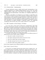
Figure 27.4 is a plot of the estimated effects estimated against the normal order scores. Random effects
will fall along a straight line on this plot. These are not statistically significant. We consider them to have
values of zero. Nonrandom effects will fall off the line; these effects will be the largest (in absolute
value). The nonrandom effects are considered to be statistically significant.
In this case a straight line covers the two- and three-factor interactions on the normal plot. None of
the interactions are significant. The significant effects are the main effects of water content, compaction
effort, and reaction time. Notice that it is possible to draw a straight line that covers the main effects and
leaves the interactions off the line. Such an interpretation — significant interactions and insignificant
main effects — is not physically plausible. Furthermore, effects of near-zero magnitude cannot be
significant when effects with larger absolute values are not.
TABLE 27.4
Effects, Plotting Positions, and Normal Order Scores for Figure 27.4
Order number i 1234567
Identity of effect 3 12 23 123 13 2 1
Effect −7.5 −2.85 −1.80 −0.35 2.05 6.40 12.45
P ==
==
100(i −−
−−
0.5)/7 0.07 0.21 0.36 0.50 0.64 0.79 0.93

Normal order scores −1.352 −0.757 −0.353 0 0.353 0.757 1.352
FIGURE 27.4 Normal probability plot of the estimated main effects and interactions.
107.9 120.8 107.6 118.9+++
4

118.6 126.5 99.8 117.5+++
4
– 1.80–=
120.8 118.6 99.8 118.9+++
4

107.9 126.5 117.5 107.6+++
4
– 0.35–=
2
-2
1
-1
0
- 10 -5 0 5 10
12
23
123
13
Effect on density
Normal Order Score
1 Water
content
3 Time
2 Compaction

effort
L1592_frame_C27.fm Page 245 Tuesday, December 18, 2001 2:47 PM
© 2002 By CRC Press LLC
The final interpretation of the results is:
1. The average density over the eight experimental design conditions is 114.7.
2. Increasing water content from 4 to 10% increases the density by an average of 12.45 lb/ft
3
.
3. Increasing compaction effort from 60 to 260 psi increases density by an average of 6.40 lb/ft
3
.
4. Increasing reaction time from 5 to 20 min decreases density by an average of 7.50 lb/ft
3
.
5. These main effects are additive because the interactions are zero. Therefore, increasing both
water content and compaction effort from their low to high values increases density by 12.45 +
6.40 = 18.85 lb/ft
3
.
Comments
Two-level factorial experiments are a way of investigating a large number of variables with a minimum
number of experiments. In general, a k variable two-level factorial experiment will require 2
k
experimental
runs. A 2
2
experiment evaluates two variables in four runs, a 2
3
experiment evaluates three variables in
eight runs, a 2

4
design evaluates four variables in sixteen runs, etc. The designs are said to be full or
saturated. From this small number of runs it is possible to estimate the average level of the response, k
main effects, all two-factor interactions, and all higher-order interactions. Furthermore, these main effects
and interactions are estimated independently of each other. Each main effect independently estimates
the change associated with one experimental factor, and only one.
Why do so few experimental runs provide so much information? The strength and beauty of this design
arise from its economy and balance. Each data point does triple duty (at least) in estimating main effects.
Each observation is used in the computation of each factor main effect and each interaction. Main effects
are averaged over more than one setting of the companion variables. This is the result of varying all
experimental factors simultaneously. One-factor-at-a-time (OFAT) designs have none of this efficiency or
power. An OFAT design in eight runs would provide only estimates of the main effects (no interactions)
and the estimates of the main effects would be inferior to those of the two-level factorial design.
The statistical significance of the estimated effects can be evaluated by making the normal plot. If the
effects represent only random variation, they will plot as a straight line. If a factor has caused an effect
to be larger than expected due to random error alone, the effect will not fall on a straight line. Effects
of this kind are interpreted as being significant. Another way to evaluate significance is to compute a
confidence interval, or a reference distribution. This is shown in Chapter 28.
Factorial designs should be the backbone of an experimenter’s design strategy. Chapter 28 shows how
four factors can be evaluated with only eight runs. Experimental designs of this kind are called fractional
factorials. Chapter 29 extends this idea. In Chapter 30 we show how the effects are estimated by linear
algebra or regression, which is more convenient in larger designs and in experiments where the inde-
pendent variables have not been set exactly according to the orthogonal design. Chapter 43 explains
how factorial designs can be used sequentially to explore a process and optimize its performance.
References
Box, G. E. P., W. G. Hunter, and J. S. Hunter (1978). Statistics for Experimenters: An Introduction to Design,
Data Analysis, and Model Building, New York, Wiley Interscience.
Box, G. E. P. and N. R. Draper (1987). Empirical Model Building and Response Surfaces, New York, John
Wiley.
Davies, O. L. (1960). Design and Analysis of Industrial Experiments, New York, Hafner Co.

Edil, T. B., P. M. Berthouex, and K. Vesperman (1987). “Fly Ash as a Potential Waste Liner,” Proc. Conf.
Geotechnical Practice in Waste Disposal, Geotech. Spec. Pub. No. 13, ASCE, pp. 447–461.
Tiao, George et al., Eds. (2000). Box on Quality and Discovery with Design, Control, and Robustness, New York,
John Wiley & Sons.
L1592_frame_C27.fm Page 246 Tuesday, December 18, 2001 2:47 PM
© 2002 By CRC Press LLC
Exercises
27.1 Recycled Water Irrigation. Evaluate an irrigation system that uses recycled water to grow cucum-
bers and eggplant. Some field test data are given in the table below. Irrigation water was applied
in two ways: sprinkle and drip. Evaluate the yield, yield per gallon, and biomass production
27.2 Water Pipe Corrosion. Students at Tufts University collected the following data to investigate
the concentration of iron in drinking water as a means of inferring water pipe corrosion. (a)
Estimate the main effects and interactions of the age of building, type of building, and location.
(b) Make the normal plot to judge the significance of the estimated effects. (c) Based on duplicate
observations at each condition, the estimate of
σ
is 0.03. Use this value to calculate the variance
of the average and the main and interaction effects. Use Var and Var(Effect) = ,
where N = total number of measurements (in this case N = 16) to evaluate the results. Compare
your conclusions regarding significance with those made using the normal plot.
27.3 Bacterial Tests. Analysts A and B each made bacterial tests on samples of sewage effluent
and water from a clean stream. The bacterial cultures were grown on two media: M1 and
M2. The experimental design is given below. Each test condition was run in triplicate. The
y values are logarithms of the measured bacterial populations. The are the variances of
the three replicates at each test condition. (a) Calculate the main and interaction effects using the
averages at each test condition. (b) Draw the normal plot to interpret the results.(c) Average
the eight variances to estimate
σ
2
for the experiment. Use = and Var(effect) =

to evaluate the results. [Note that Var(effect) applies to main effects and interactions. These
variance equations account for the replication in the design.]
Vegetable
Irrigation
Type
Irrigation
Source
Yield
(lb/ft
2
)
Yield
(lb/gal)
Biomass
(lb/plant)
Cucumber Sprinkle Tap water 6.6 0.15 5.5
Recycled water 6.6 0.15 5.7
Drip Tap water 4.9 0.25 4.5
Recycled water 4.8 0.25 4.0
Eggplant Sprinkle Tap water 2.9 0.07 3.0
Recycled water 3.2 0.07 3.5
Drip Tap water 1.6 0.08 1.9
Recycled water 2.3 0.12 2.3
Age Type Location Iron (mg/L)
Old Academic Medford 0.23 0.28
New Academic Medford 0.36 0.29
Old Residential Medford 0.03 0.06
New Residential Medford 0.05 0.02
Old Academic Somerville 0.08 0.05
New Academic Somerville 0.03 0.08

Old Residential Somerville 0.04 0.07
New Residential Somerville 0.02 0.06
Source Analyst Medium y (3 Replicates)
Effluent A M1 3.54 3.79 3.40 3.58 0.0390
Stream A M1 1.85 1.76 1.72 1.78 0.0044
Effluent B M1 3.81 3.82 3.79 3.81 0.0002
Stream B M1 1.72 1.75 1.55 1.67 0.0116
Effluent A M2 3.63 3.67 3.71 3.67 0.0016
Stream A M2 1.60 1.74 1.72 1.69 0.0057
Effluent B M2 3.86 3.86 4.08 3.93 0.0161
Stream B M2 2.05 1.51 1.70 1.75 0.0750
y() S
p
2
/N= 4S
p
2
/N
s
i
2
Var y()
σ
2
24

σ
2
6
-

y
i
s
i
2
L1592_frame_C27.fm Page 247 Tuesday, December 18, 2001 2:47 PM
© 2002 By CRC Press LLC
27.4 Reaeration. The data below are from an experiment that attempted to relate the rate of disso-
lution of an organic chemical to the reaeration rate (y) in a laboratory model stream channel.
The three experimental factors are stream velocity (V, in m/sec), stream depth (D, in cm), and
channel roughness (R). Calculate the main effects and interactions and interpret the results.
27.5 Metal Inhibition. The results of a two-level, four-factor experiment to study the effect of zinc
(Zn), cobalt (Co), and antimony (Sb) on the oxygen uptake rate of activated sludge are given
below. Calcium (Ca) was added to some test solutions. The (−) condition is absence of Ca,
Zn, Co, or Sb. The (+) condition is 10 mg/L Zn, 1 mg/L Co, 1 mg/L Sb, or 300 mg/L Ca (as
CaCO
3
). The control condition (zero Ca, Zn, Co, and Sb) was duplicated. The measured
response is cumulative oxygen uptake (mg/L) in 20-hr reaction time. Interpret the data in
terms of the main and interaction effects of the four factors.
27.6 Plant Lead Uptake. Anaerobically digested sewage sludge and commercial fertilizer were
applied to garden plots (10 ft × 10 ft) on which were grown turnips or Swiss chard. Each
treatment was done in triplicate. After harvesting, the turnip roots or Swiss chard leaves were
washed, dried, and analyzed for total lead. Determine the main and interaction effects of the
sludge and fertilizer on lead uptake by these plants.
Run V D R y (Triplicates) Average
1 0.25 10 Smooth 107 117 117 113.7
2 0.5 10 Smooth 190 178 179 182.3
3 0.25 15 Smooth 119 116 133 122.7

4 0.5 15 Smooth 188 191 195 191.3
5 0.25 10 Coarse 119 132 126 125.7
6 0.5 10 Coarse 187 173 166 175.3
7 0.25 15 Coarse 140 133 132 135.0
8 0.5 15 Coarse 164 145 144 151.0
Run Zn Co Sb Ca
Uptake
(mg/L)
1 −1 −1 −1 −1 761
2 +1 −1 −1 −1 532
3 −1 +1 −1 −1 759
4 +1 +1 −1 −1 380
5 −1 −1 +1 −1 708
6 +1 −1 +1 −1 348
7 −1 +1 +1 −1 547
8 +1 +1 +1 −1 305
9 −1 −1 −1 +1 857
10 +1 −1 −1 +1 902
11 −1 +1 −1 +1 640
12 +1 +1 −1 +1 636
13 −1 −1 +1 +1 822
14 +1 −1 +1 +1 798
15 −1 +1 +1 +1 511
16 +1 +1 +1 +1 527
1 (rep) −1 −1 −1 −1 600
Source: Hartz, K. E., J. WPFC, 57, 942–947.
Exp. Sludge Fertilizer Turnip Root Swiss Chard Leaf
1 None None 0.46, 0.57, 0.43 2.5, 2.7, 3.0
2 110 gal/plot None 0.56, 0.53, 0.66 2.0, 1.9, 1.4
3 None 2.87 lb/plot 0.29, 0.39, 0.30 3.1, 2.5, 2.2

4 110 gal/plot 2.87 lb/plot 0.31, 0.32, 0.40 2.5, 1.6, 1.8
Source: Auclair, M. S. (1976). M.S. thesis, Civil Engr. Dept., Tufts University.
L1592_frame_C27.fm Page 248 Tuesday, December 18, 2001 2:47 PM
© 2002 By CRC Press LLC

28

Fractional Factorial Experimental Designs

KEY WORDS

alias structure, confounding, defining relation, dissolved oxygen, factorial design, frac-
tional factorial design, half-fraction, interaction, main effect, reference distribution, replication, ruggedness
testing,

t

distribution, variance.

Two-level factorial experimental designs are very efficient but the number of runs grows exponentially
as the number of factors increases.
3 factors at 2 levels 2

3



=

8 runs

4 factors at 2 levels 2

4



=

16 runs
5 factors at 2 levels 2

5



=

32 runs
6 factors at 2 levels 2

6



=

64 runs
7 factors at 2 levels 2

7

=

128 runs
8 factors at 2 levels 2

8



=

256 runs
Usually your budget cannot support 128 or 256 runs. Even if it could, you would not want to commit your
entire budget to one very large experiment. As a rule-of-thumb, you should not commit more than 25% of the
budget to preliminary experiments for the following reasons. Some of the factors may be inactive and you
will want to drop them in future experiments; you may want to use different factor settings in follow-up
experiments; a two-level design will identify interactions, but not quadratic effects, so you may want to augment
the design and do more testing; you may need to repeat some experiments; and/or you may need to replicate
the entire design to improve the precision of the estimates. These are reasons why

fractional factorial designs

are attractive. They provide flexibility by reducing the amount of work needed to conduct preliminary exper-
iments that will screen for important variables and guide you toward more interesting experimental settings.

Fractional

means that we do a fraction or a part of the full factorial design. We could do a half-fraction,
a quarter-fraction, or an eighth-fraction. A half-fraction is to do half of the full factorial design, or
(1

/

2)2

4



=

(1

/

2)16

=

8 runs to investigate four factors; (1

/

2)(2

5

)

=

(1

/

2)32

=

16 runs to investigate five factors;
and so on. Examples of quarter-fractions are (1

/

4)2

5



=

(1

/

4)32

=

8, or (1

/

4)2

7



=

(1

/

4)128

=

32 runs. An
example eighth-fraction is (1

/

8)2

8



=

(1

/

8)256

=

32 runs. These five examples lead to designs that could
investigate 4 variables in 8 runs, 5 factors in 16 runs or 8 runs, 7 factors in 32 runs, or 8 factors in 32 runs.
Of course, some information must be sacrificed in order to investigate 8 factors in 32 runs, instead of
the full 256 runs, but you will be surprised how little is lost. The lost information is about interactions,
if you select the right 32 runs out of the possible 2

8



=

256. How to do this is explained fully in Box et al.
(1978) and Box and Hunter (1961a, 1961b).

Case Study: Sampling High Dissolved Oxygen Concentrations

Ruggedness testing

is a means of determining which of many steps in an analytical procedure must be
carefully controlled and which can be treated with less care. Each aspect or step of the technique needs
checking. These problems usually involve a large number of variables and an efficient experimental
approach is needed. Fractional factorial designs provide such an approach.

L1592_frame_C28.fm Page 249 Tuesday, December 18, 2001 2:48 PM
© 2002 By CRC Press LLC

It was necessary to measure the oxygen concentration in the influent to a pilot plant reactor. The influent
was under 20 psig pressure and was aerated with pure oxygen. The dissolved oxygen (DO) concentration
was expected to be about 40 mg

/

L. Sampling methods that are satisfactory at low DO levels (e.g., below
saturation) will not work in this situation. Also, conventional methods for measuring dissolved oxygen
are not designed to measure DO above about 20 mg

/

L. The sampling method that was developed involved
withdrawing the highly oxygenated stream into a volume of deoxygenated water, thereby diluting the DO
so it could be measured using conventional methods. The estimated

in situ

DO of the influent was the

measured DO multiplied by the dilution factor.
There was a possibility that small bubbles would form and oxygen would be lost as the pressure
dropped from 20 psig in the reactor to atmospheric pressure in the dilution bottle. It was essential to
mix the pressurized solution with the dilution water in a way that would eliminate, or at least minimize,
this loss. One possible technique would be to try to capture the oxygen before bubbles formed or escaped
by introducing the sample at a high rate into a stirred bottle containing a large amount of dilution water.
On the other hand, the technique would be more convenient if stirring could be eliminated, if a low
sample flow rate could be used, and if only a small amount of dilution water was needed. Perhaps one
or all of these simplifications could be made. An experiment was needed that would indicate which of
these variables were important in a particular context. The outcome of this experiment should indicate
how the sampling technique could be simplified without loss of accuracy.
Four variables in the sampling procedure seemed critical: (1) stirring rate S, (2) dilution ratio D, (3)
specimen input location L, and (4) sample flow rate F. A two-level, four-variable fractional factorial
design (2

4

−

1

) was used to evaluate the importance of the four variables. This design required measurements
at eight combinations of the independent variables. The high and low settings of the independent variables
are shown in Table 28.1. The experiment was conducted according to the design matrix in Table 28.2,
where the factors (variables) S, D, L, and F are identified as 1, 2, 3, and 4, respectively. The run order
was randomized, and each test condition was run in duplicate. The average and difference between
duplicates for each run are shown in Table 28.2.

TABLE 28.1

Experimental Settings for the Independent Variables

Setting
Stirring
S
Dilution
Ratio D
Sample Input
Location L
Sample Flow
Rate F

Low level (

−

) Off 2:1 Surface 2.6 mL/sec
High level (

+

) On 4:1 Bottom 8.2 mL/sec

TABLE 28.2

Experimental Design and Measured Dissolved Oxygen Concentrations

Duplicates (mg/L)
Avg. DO (mg/L) Difference (mg/L)
Run S (1) D (2) L (3) F (4)

y

1

i

y

2

i

d

i

1

−−−−

38.9 41.5 40.20

−

2.6
2

+−−+

45.7 45.4 45.55 0.3
3

−+−+

47.8 48.8 48.30

−

1.0
4

++−−

45.8 43.8 44.80 2.0
5

−−++

45.2 47.6 46.40

−

2.4
6

+−+−

46.9 48.3 47.60

−

1.4
7

−++−

41.0 45.8 43.40

−

4.8
8

++++

53.5 52.4 52.95 1.1

Note:

Defining relation:

I

=

1234

.
y

i

L1592_frame_C28.fm Page 250 Tuesday, December 18, 2001 2:48 PM
© 2002 By CRC Press LLC

Method: Fractional Factorial Designs

A fractional factorial design

is an experimental layout where a full factorial design is augmented with
one or more factors (independent variables) to be analyzed without increasing the number of experimental
runs. These designs are labeled 2

k

−

p

, where

k

is the number of factors that could be evaluated in a full
factorial design of size 2

k

and

p

is the number of additional factors to be included. When a fourth factor
is to be incorporated in a 2

3

design of eight runs, the resulting design is a 2

4

−

1

fractional factorial, which
also has 2

3



=

8 runs. The full 2

4

factorial would have 16 runs. The 2

4

−

1

has only eight runs. It is a half-
fraction of the full four-factor design. Likewise, a 2

5

−

2

experimental design has eight runs; it is a quarter-
fraction of the full five-factor design.
To design a half-fraction of the full four-factor design, we must determine which half of the 2

4



=

16
experiments is to be done. To preserve the balance of the design, there must be four experiments at the
high setting of

X

4

and four experiments at the low setting. Note that any combination of four high and four
low that we choose for factor 4 will correspond exactly to one of the column combinations for interactions
among factors

X

1

,

X

2

, and

X

3

already used in the matrix of the 2

3

factorial design (Table 28.2). Which

combination should we select? Standard procedure is to choose the three-factor interaction

X

1

X

2

X

3

for
setting the levels of

X

4

. Having the levels of

X

4

the same as the levels of

X

1

X

2

X

3

means that the separate
effects of

X

4

and

X

1

X

2

X

3

cannot be estimated. We can only estimate their combined effect. Their individual
effects are confounded.

Confounded

means confused with, or tangled up with, in a way that we cannot
separate without doing more experiments.
The design matrix for a 2

4

−

1

design is shown in Table 28.3. The signs of the factor 4 column vector
of levels are determined by the product of column vectors for the column 1, 2, and 3 factors. (Also, it
is the same as the three-factor interaction column in the full 2

3

design.) For example, the signs for run
4 (row 4) are (

+

) (

+

) (

−

) (

−

), where the last (

−

) comes from the product (

+

) (

+

) (

−

)

=

(

−

).
The model matrix is given in Table 28.4. The eight experimental runs allow estimation of eight effects,
which are computed as the product of a column vector

X

i

and the

y

vector just as was explained for the
full factorial experiment discussed in Chapter 27. The other effects also are computed as for the full
factorial experiment but they have a different interpretation, which will be explained now.
To evaluate four factors with only eight runs, we give up the ability to estimate independent main
effects. Notice in the design matrix that column vector

1

is identical to the product of column vectors

2

,

3

, and 4. The effect that is computed as y · X
1
is not an independent estimate of the main effect of
factor 1. It is the main effect of X
1
plus the three-way interaction of factors 2, 3, and 4. We say that the
main effect of X
1
is confounded with the three-factor interaction of X
2
, X
3
, and X
4
. Furthermore, each
main effect is confounded with a three-factor interaction, as follows:
1 + 234 2 + 134 3 + 124 4 + 123
The defining relation of the design allows us to determine all the confounding relationships in the
fractional design. In this 2
4−1
design, the defining relation is I = 1234. I indicates a vector of +1’s.
TABLE 28.3
Design Matrix for a 2
4−1
Fractional Factorial Design
Factor (Independent Variable)
Run1234
1 −−−−

2 +−−+
3 −+−+
4 ++−−
5 −−++
6 +−+−
7 −++−
8 ++++
L1592_frame_C28.fm Page 251 Tuesday, December 18, 2001 2:48 PM
© 2002 By CRC Press LLC
Therefore, I = 1234 means that multiplying the column vectors for factors 1, 2, 3, and 4, which consists
of +1’s and −1’s, gives a vector that consists of +1 values. It also means that multiplying the column
vectors of factors 2, 3, and 4 gives the column vector for factor 1. This means that the effect calculated
using the column of +1 and
−1 values for factor 1 is the same as the value that is calculated using the
column vector of the X
2
X
3
X
4
interaction. Thus, the main effect of factor 1 is confounded with the three-
factor interaction of factors 2, 3, and 4. Also, multiplying the column vectors of factors 1, 3, and 4 gives
the column vector for factor 2, etc.
Having the main effects confounded with three-factor interactions is part of the price we pay we to
investigate four factors in eight runs. Another price, which can be seen in the defining relation I = 1234,
is that the two-factor interactions are confounded with each other:
12 + 34 13 + 24 23 + 14
The two-way interaction of factors 1 and 2 is confounded with the two-way interaction of factors 3 and
4, etc.
The consequence of this intentional confounding is that the estimated main effects are biased unless

the three-factor interactions are negligible. Fortunately, three-way interactions are often small and can
be ignored. There is no safe basis for ignoring any of the two-factor interactions, so the effects calculated
as two-factor interactions must be interpreted with caution.
Understanding how confounding is identified by the defining relation reveals how the fractional design
was created. Any fractional design will involve some confounding. The experimental designer wants to
make this as painless as possible. The best we can do is to hope that the three-factor interactions are
unimportant and arrange for the main effects to be confounded with three-factor interactions. Intentionally
confounding factor 4 with the three-factor interaction of factors 1, 2, and 3 accomplishes that. By convention,
we write the design matrix in the usual form for the first three factors. The fourth column becomes the
product of the first three columns. Then we multiply pairs of columns to get the columns for the two-factor
interactions, as shown in Table 28.4.
Case Study Solution
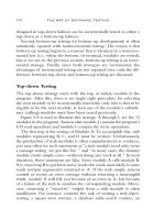
The average response at each experimental setting is shown in Figure 28.1. The small boxes identify
the four tests that were conducted at the high flow rate (X
4
); the low flow rate tests are the four unboxed
values. Calculation of the effects was explained in Chapter 27 and are not repeated here. The estimated
effects are given in Table 28.5.
This experiment has replication at each experimental condition so we can estimate the variance of the
measurement error and of the estimated effects. The differences between duplicates (d
i
) can be used to
TABLE 28.4
Model Matrix for the 2
4−1
Fractional Factorial Design
1234 ==
==
123 12 ==
==

34 13 ==
==
24 23 ==
==
14
Run Avg. S D L F (SDL) SD (LF) SL (DF) DL (SF)
1 +−−−−+++
2 ++−−+−−+
3 +−+ − +− + −
4 +++−−+−−
5 +−−+++−−
6 ++−+−−+−
7 +−++−−−+
8 ++++++++
Note: Defining relation: I = 1234 (or I = SDLF).
L1592_frame_C28.fm Page 252 Tuesday, December 18, 2001 2:48 PM
© 2002 By CRC Press LLC
estimate the variance of the average response for each run. For a single pair of duplicate observations
(y
1i
and y
2i
), the sample variance is:

where d
i
= y
1i
− y
2i

is the difference between the two observations. The average of the duplicate observ-
ations is:
and the variance of the average of the duplicates is:
The individual estimates for n pairs of duplicate observations can be combined to get a pooled estimate
of the variance of the average:
FIGURE 28.1 A 2
4−1
fractional factorial design and the average of duplicated measurements at each of the eight design
settings.
TABLE 28.5
Estimated Effects and Their Standard Errors
Effect
Contributing
Factors and
Interactions
Estimated
Effect
Estimated
Standard Error

Average + 1234 Average(I) + SDLF 46.2 0.41
1 + 234 S + DLF 3.2 0.82
2 + 134 D + SLF 2.4 0.82
3 + 124 L + SDF 2.9 0.82
4 + 123 F + SDL 4.3 0.82
12 + 34 SD + LF −0.1 0.82
13 + 24 SL + DF 2.2 0.82
23 + 14 DL + SF −1.2 0.82
48.3
45.6

43.4
46.4
53.0
2:1
4:1 44.8
47.6
40.2
Dilution
ratio
off Stirring on
Input
Location
bottom
top
s
i
2
1
2

d
i
2
=
y
i
y
1i
y
2i

–
2

=
s
y
2
s
i
2
2

d
i
2
4

==
s
y
2
1
n

d
i
2
4

i=1

n
∑
1
4n

d
i
2
i=1
n
∑
==
L1592_frame_C28.fm Page 253 Tuesday, December 18, 2001 2:48 PM
© 2002 By CRC Press LLC
For this experiment, n = 8 gives:
and
The main and interaction effects are estimated using the model matrix given in Table 28.4. The average is:
and the estimate of each effect is:
where X
ij
is the ith element of the vector in column j.
The variance of the average is:
and the variance of the main and interaction effects is:
Substituting for gives the standard errors of the average and the estimated effects:
and
The estimated effects and their standard errors are given in Table 28.5.
The 95% confidence interval for the true value of the effects is bounded by:
Effect
j
± t

ν
=8,
α
/2 =0.025
SE (Effect
j
)
Effect
j
± 2.306(0.82) = Effect
j
± 1.9
from which we can state, with 95% confidence, that effects larger than 1.9, or smaller than −1.9, represent
real effects. All four main effects and the two-factor interaction SL + DF are significant.
Alternately, the estimated effects can be viewed in relation to their relevant reference distribution
shown in Figure 28.2. This distribution was constructed by scaling a t distribution with
ν
= 8 degrees
of freedom according to the estimated standard error of the effects, which means, in this case, using a
scaling factor of 0.83. The calculations are shown in Table 28.6.
The main effects of all four variables are far out on the tails of the reference distribution, indicating
that they are statistically significant. The bounds of the confidence interval (±1.9) could be plotted on
this reference distribution, but this is not necessary because the results are clear. Stirring (S), on average,
s
y
2
1
48()

2.6–()

2
0.3
2
…
1.1
2
+++()1.332==
s
y
1.15=
y
1
8

y
i
i=1
8
∑
=
Effect j()
1
4

X
ij
y
i
i=1
8

∑
=
y
Var y() 1/8()
2
8
σ
y
2
σ
y
2
8

==
Var Effect()1/4()
2
8
σ
y
2
σ
y
2
2

==
s
y
2

σ
y
2
SE y()
s
y
2
8

1.332
8
0.41== =
SE Effect
j
()
s
y
2
2

1.332
2
0.82== =
L1592_frame_C28.fm Page 254 Tuesday, December 18, 2001 2:48 PM
© 2002 By CRC Press LLC
elevates the response by 3.2 mg/L. Changing the dilution rate (D) from 2:1 to 4:1 causes an increase of
2.4 mg/L. Setting the sample input location (L) at the bottom yields a response 2.9 mg/L higher than a
surface input location. And, increasing the sample flow rate (F) from 2.6 to 8.2 mL/sec causes an increase
of about 4.3 mg/L.
Assuming that the three-factor interactions are negligible, the effects of the four main factors S, D, L,

and F can be interpreted as being independent estimates (that is, free of confounding with any interactions).
This assumption is reasonable because significant three-factor interactions rarely exist. By this we mean
that it is likely that three interacting factors will have a tendency to offset each other and produce a combined
effect that is comparable to experimental error. Thus, when the assumption of negligible three-factor
interaction is valid, we achieve the main effects from eight runs instead of 16 runs in the full 2
4
factorial.
The two-factor interactions are confounded pairwise. The effect we have called DL is not the pure
interaction of factors D and L. It is the interaction of D and L plus the interaction of S and F. This same
problem exists for all three of the two-factor interaction effects. This is the price of running a 2
4−1
fractional factorial experiment in eight runs instead of the full 2
4
design, which would estimate all effects
without confounding.
Whenever a two-factor interaction appears significant, interpretation of the main effects must be
reserved until the interactions have been examined. The reason for this is that a significant two-factor
interaction means that the main effect of one interacting factor varies as a function of the level of the
other factor. For example, factor X
1
might have a large positive effect at a low value of X
2
, but a large
negative effect at a high value of X
2
. The estimated main effect of X
1
could be near zero (because of
TABLE 28.6
Constructing the Reference Distribution for Scale Factor =

0.82
t distribution (
ν
==
==
8) Scaled Reference Distribution
a
Value of t t Ordinate t ××
××
0.82 Ordinate/0.82
0 0.387 0.00 0.472
0.25 0.373 0.21 0.455
0.5 0.337 0.41 0.411
0.75 0.285 0.62 0.348
1.0 0.228 0.82 0.278
1.25 0.173 1.03 0.211
1.50 0.127 1.23 0.155
1.75 0.090 1.44 0.110
2.00 0.062 1.64 0.076
2.25 0.043 1.85 0.052
2.50 0.029 2.05 0.035
2.75 0.019 2.26 0.023
3.0 0.013 2.46 0.016
a
Scaling both the abscissa and the ordinate makes the area under the
reference distribution equal to 1.00.
FIGURE 28.2 Reference distribution that would describe the effects and interactions if they were all random. Effects or
interactions falling on the tails of the reference distribution are judged to be real.
-4 -3 -2 -1 0 +1 +2 +3 +4 +5
Effects and Interactions (mg/L DO)

SD+ LF
D L S F
SL + DF
DL + SF
L1592_frame_C28.fm Page 255 Tuesday, December 18, 2001 2:48 PM
© 2002 By CRC Press LLC
averaging the positive and negative effects) and looking at it alone might lead us to wrongly conclude
that the factor is inactive.
In this case study, the SL + DF interaction effect appears large enough to be real. Interpreting the SL
interaction is done by viewing the experiment as one conducted in the interacting factors only. This is
shown in Figure 28.3, where the responses averaged over all runs with the same signs for L and S. The
same examination must be made of the DF interaction, which is also shown in Figure 28.3.
The sample flow rate is not very important at the low dilution ratio and dilution ratio is not very
important at the low sample flow rate. But when the sample flow rate is high and the dilution ratio is
large, the response increases dramatically. A similar interpretation can be made for the SL interaction.
Stirring in conjunction with injecting the sample at the bottom gives higher oxygen measurements while
the other three combinations of L and S show much the same DO levels.
In short, the significant two-factor interaction means that the effect of any factor depends on the level
of some other factor. It may be, however, that only one of the interactions SL or DF is real and the other
is an artifact caused by the confounding of the two interactions. Additional experiments could be done
to untangle this indefinite situation. One option would be to run the other half of the 2
4−1
design.
For the case study problem, a resolution of the two-factor interaction is not needed because all four factors
S, D, L, and F do influence the oxygen measurements and it is clear that all four should be set at their +
levels. That is, the best of the measurement techniques investigated would be to inject the sample at the
bottom of the bottle, stir, use the 4:1 dilution ratio, and use the high sample flow rate (8.2 mL/sec). Using
even higher dilution ratios, faster stirring, and a higher sample flow rate might yield even better results.
Comments
This example has shown how four variables can be evaluated with just eight runs. The eight runs were

a half-fraction of the sixteen runs that would be used to evaluate four factors in a full factorial design.
This design provided estimates of the main effects of the four factors just as would have been obtained
from the full 2
4
design, if we are willing to make the rather mild assumption that three-factor interactions
are negligible.
There was a price paid for forcing the extra factor into the eight-run design. Only a total of eight
effects and interactions can be estimated from the eight runs. These include the average and the four
main effects. The estimated two-factor interactions are confounded pairwise with each other and their
interpretation is not as clear as it would have been from the full factorial design.
Often we are interested primarily in the main effects, at least in the early iterations of the learning
cycle. If the main effects are significant and some of the two-factor interactions hold interest, additional
runs could be performed to untangle the interpretation. The most logical follow-up experiment would
be to run the other half of the 2
4−1
design. Table 28.7 shows how the full 2
4
design was divided into two
half-fractions, one of which was used in the case study experiment, and the other which could be used
as a follow-up. The two half-fractions combined are a saturated 2
4
design from which all main effects
and all interactions can be estimated independently (i.e., without confounding). A further advantage is
that the two half-fractions are blocks and any nuisance factors that enter the experiment between the
execution of the half-fractions will not distort the final results. (This is not obvious. For details, see Box
et al., 1978.)
FIGURE 28.3 Two-factor interactions of S and L, and of F and D.
(–) (+)
45.(+) 944.9 50.3
(+) 50.6

43.9(–)
(–) (+)
45.144.25(–) 44.1
Input
Location
Flow
Rate
Stirring Dilution
Ratio
L1592_frame_C28.fm Page 256 Tuesday, December 18, 2001 2:48 PM
© 2002 By CRC Press LLC
Fractional factorial designs are often used in an iterative experimental strategy. Chapter 29 illustrates
a 2
5−1
design for evaluating five factors in 16 runs. Box et al. (1978) give two examples of 2
7−4
designs
for evaluating eight variables in 2
3
= 8 runs. They also show other fractional factorial designs, their
confounding pattern, and give a detailed explanation of how the confounding pattern is discovered.
References
Box, G. E. P. and J. S. Hunter (1961a). “The 2
k−p
Fractional Factorial Designs. Part I,” Technometrics, 3(3),
311–351.
Box, G. E. P. and J. S. Hunter (1961b). “The 2
k−p
Fractional Factorial Designs. Part II,” Technometrics, 3(4),
449–458.

Box, G. E. P., W. G. Hunter, and J. S. Hunter (1978). Statistics for Experimenters: An Introduction to Design,
Data Analysis, and Model Building, New York, Wiley Interscience.
Tiao, George et al., Eds. (2000). Box on Quality and Discovery with Design, Control, and Robustness, New York,
John Wiley & Sons.
Exercises
28.1 Membrane Bioreactor. The ZeeWeed internal-membrane reactor was tested using a 2
4−1
fractional factorial design to evaluate four factors in eight runs, as shown in the table below.
The response is the permeate flow rate. Evaluate the main effects and interactions.
TABLE 28.7
Two Half-Fractions of the Full 2
4
Factorial Design
Factor
12 34
I - Run 1 −− −−
II + – −−
II −+ −−
I - Run 4 ++ −−
II −− +−
I - Run 6 +− +−
I - Run 7 −+ +−
II ++ +−
II −− −+
I - Run 2 +− −+
I - Run 3 −+ −+
II ++ −+
I - Run 5 −− ++
II +− ++
II −+ ++

I - Run 8 ++ ++
Note: The eight settings opposite I - Run 1, I - Run 2, etc. were used in the
2
4−1
fractional design of the case study. The other eight combinations, marked
II, are a second 2
4−1
fractional design that could be run as a follow-up.
Backpulse Backpulse Membrane Permeate
Duration Frequency Airflow MLSS Flow Rate
(min) (min) (m
3
/hr) (mg/L) (L/min)
−1 −1 −1 −183
+1 −1 −1 +172
−1 +1 −1 +164
+1 +1 −1 −172
L1592_frame_C28.fm Page 257 Tuesday, December 18, 2001 2:48 PM
© 2002 By CRC Press LLC
28.2 Corrosion. A study of the effect of construction metal corrosion under simulated acid fog/rain
conditions used factorial experimental designs with pH, salinity, temperature, and exposure
time as variables. The 2
4−1
experiment was performed on galvanized steel and the response
was corrosion rate. Each run was replicated n = 17 times. Estimate the main effects of the four
factors and the two-factor interactions. Note that the design identity is I ==
==
1234, so the two-
factor interactions are confounded with other two-factor interactions.
28.3 Fly Ash Mixture. The table below describes a 2

5−1
experiment in 16 runs to investigate five
factors: (1) type of fly ash, (2) percentage fly ash in the mixture, (3) test specimens put
through a wet/dry curing cycle, (4) test specimens put through a freeze/thaw curing cycle,
and (5) percentage of bentonite in the mixture. High permeability is desirable. What combi-
nation of factors promotes this? Quantify the effect of the five factors. Evaluate and explain
any interactions between factors.
28.4 Metal Inhibition. Divide the 2
4
factorial experiment in Exercise 27.5 into two half-fractions.
Calculate the main effects and interactions of each half-fraction and compare them.
−1 −1 +1 +164
+1 −1 +1 −187
−1 +1 +1 −181
+1 +1 +1 +168
Note: Defining relation: I = 1234.
Source: Cantor, J. et al. (1999). Ind. Wastewater, Nov./Dec., pp. 18–22.
Salinity Temp. Time Avg. Corrosion St. Dev.
Run pH (%NaCl) (°°
°°
C) (hr) Rate (
µµ
µµ
m/yr) (
µµ
µµ
m/yr)
1 2.5 1.0 35 48 501 65
2 3.5 1.0 35 120 330 60
3 2.5 6.0 35 120 561 67

4 3.5 6.0 35 48 666 95
5 2.5 1.0 45 120 218 85
6 3.5 1.0 45 48 247 57
7 2.5 6.0 45 48 710 102
8 3.5 6.0 45 120 438 51
Source: Fang, H. H. P. et al. (1990). Water, Air, and Soil Poll., 53, 315–325.
Run
Type of
Fly Ash
Fly Ash
(%)
Wet/Dry
Cycle
Freeze/Thaw
Cycle
Bentonite
(%) Permeability
1 A 50 N N 10 1000
2 B 50 N N 0 160
3 A 100 N N 0 1450
4 B 100 N N 10 77
5 A 50 Y N 0 1400
6 B 50 Y N 10 550
7 A 100 Y N 10 320
8 B 100 Y N 0 22
9 A 50 N Y 0 1400
10 B 50 N Y 10 390
11 A 100 N Y 10 580
12 B 100 N Y 0 8
13 A 50 Y Y 10 2800

14 B 50 Y Y 0 160
15 A 100 Y Y 0 710
16 B 100 Y Y 10 19
L1592_frame_C28.fm Page 258 Tuesday, December 18, 2001 2:48 PM
© 2002 By CRC Press LLC
28.5 Water Pipe Corrosion. Environmental engineering students at Tufts University performed a
2
4−1
fractional factorial experiment to investigate the concentration of iron in drinking water
in various campus buildings as a means of inferring water pipe corrosion. The four experimental
factors were age of building, building type, location, and day of week. Estimate the main and
interaction effects and their 95% confidence intervals. The design identity is I ==
==
1234, and the
results are:
Age Type Location Day Iron (mg/L)
Old Academic Medford Wednesday 0.26, 0.21
New Academic Medford Monday 0.37, 0.32
Old Residential Medford Monday 0.01, 0.05
New Residential Medford Wednesday 0.03, 0.07
Old Academic Somerville Monday 0.11, 0.05
New Academic Somerville Wednesday 0.06, 0.03
Old Residential Somerville Wednesday 0.03, 0.05
New Residential Somerville Monday 0.07, 0.02
L1592_frame_C28.fm Page 259 Tuesday, December 18, 2001 2:48 PM