A Guide to Microsofl Excel 2002 for Scientists and Engineers phần 3 ppsx

Using Functions
Concepts
Microsoft Excel provides over 300 worksheet functions which
are
. divided into
10
groups: mathematical and trigonometric,
engineering, logical, statistical, date and time, database, financial,
informational, lookup and reference, and text. In addition, the user
may construct user-defined (custom) functions
-
see
Chapter
8.
is required
for
the Engineering
hnctions
to
be available.
Suppose you wish
to
know the value of Log(3). We call 3 the
argument
of the function. It is the value that is used by the function
to compute the required quantity. Some functions take more than
one argument. We say that a function
returns
a value. The
syntax
of a function are the rules for its use.

Figure 4.1 illustrates a formula using a function. The MAX
function returns the value of the largest argument. The formula in
the figure will return the larger of the value in Al, one of the
values in the range
B1
:B8
or the constant value
10.
In this example
the arguments are a cell reference,
a
range reference and a
constant.
Equal sign when function begins formula
Function name
=MAX(AI,
BI:B8,
IO)
Commas separate each argument
Arguments are enclosed in parentheses
No
space is permitted between the name
and the opening parenthesis
Figure
4.1
56
A
Guide to Microsoft Excel
2002
for Scientists

and
Engineers
Depending on the function, the number of arguments may be fixed,
variable or even zero. For example:
zero arguments
=PI()
one argument
=SQRT(A2)
or
=SQRT(A2/2)
two
arguments
=ROUND(A2,2)
variable number
=SUM(AI :A10)
or
=SUM(AI :AIO,B3,B4)
When the number of permitted arguments
is variable, the
maximum number is
30
and the number of characters may not
exceed
1024.
Note that a range such as
AI
:A1
00
counts as one
argument, not

100.
While some functions require specific types of arguments, most
functions permit an argument to be a cell reference, a range
reference, a constant, an expression or another function. Certain
functions require text type arguments and others require logical
arguments. For example:
Cell and range
=SUM(AI, B1:BIO)
Named range
=SUM(Xvalues)
Cell and constant
=MAX(AI,
20)
Constant
=LOG10(9.81)
Expression
=LOGlO(A1/2)
Function
=SIN(RADIANS(AI
))
When a function
is
used as an argument we use the term
nesting.
Functions may be nested up to seven levels.
An
example of three-
level nesting
is
=LOGIO(MAX (SUM(A1 :A4),25)).

To
interpret this
we read from the inside. First the range
A1
:A4 is summed, then
Excel determines the maximum
of
the sum and the value
25
and,
finally, computes the base
10
logarithm
of
the result of that
determination.
Formulas may be constructed from cell references, constants and
functions. For example:
=2*PI()
returns
2n
=2.5*SUM(AI
:MO)/SQRT(Bl)
formula with two functions
and a constant
Spaces may be used in a formula to make it more readable.
This
includes spaces on each side of an arithmetical operator,
or
on

either side of the commas separating arguments
in
a function call.
You may
not
have
a
space between the function name and the
opening parenthesis; you will be rewarded with a #NAME? error.
Using Functions
5
7
There
is
not room
in this book to discuss all the worksheet
functions.
A
list of the functions
in
the various categories can be
found by using Helplcontents and then expanding
Function
Reference.
You
should review the lists before constructing a
complex formula
or
worksheet.
For

example, suppose
A
1
:A
1
0
contains some numeric values and you wish to find the sum
of
the
squares ofthese values.
You
may be tempted
to
use
BI
:B10
to hold
the squared values and then sum that range. However, Excel
provides a function
to
compute this value; use Help to find its
name.
Some functions are described as
array
functions
and need to be
entered in
a
special manner. We examine some of these later.
A

number of errors can arise with formulas and functions. When
this happens, Excel displays one of these error values.
#DIV/O!
Division by zero.
#NAME?
A
formula contains an undefined variable or
function name,
or
a space between the name of a
function and the opening parenthesis.
#N/A
No
value
is
available.
#NULL!
A
result has no value.
#NUM!
Numeric overflow;
e.g. a cell with
=SQRT(Zl)
when
Z1
has a
negative value
#REF!
Invalid cell reference.
#VALUE! Invalid argument type;

e.g. a cell with
=LN(ZI)
when
Z1
contains text.
When a cell having an error value
is
referenced in the formula of
a second cell, that cell will also have an error value.
An error you are sure to meet once or twice
is
the
circular
reference
error.
A
formula cannot contain a reference to the cell
address of its
own
location.
For
example, it would be meaningless
to place in
A10
the formula
=SUM(Al:AlO).
If you
try
this, Excel
displays an error dialog box with

Cannot resolve circular
reference.
If
you click
OK,
the Circular Reference tool appears to
help you find the source of the problem.
An
uncorrected circular
reference results in a message
in
the
status
bar in the form
Circular:
AI0
to warn you
of
the problem. There are some
specialized uses for circular references, one of which is shown
in
a later chapter.
58
A
Guide to Microsoft Excel
2002
for Scientists
and
Engineers
Exercise

1
:
Autosum
At the completion of the next three exercises, your worksheet
should resemble that in Figure 4.2.
and AutoCalculate
Figure
4.2
(b)
NlAutoSum tool pre-Excel2002
HAutoSum
tool
in
Excel 2002
Open a new workbook. Enter the values shown in A1 :A3 and
the text in C
1
:C3.
Select the cell A4 and click the AutoSum button
on
the
Standard toolbar. AutoSum will select the range A1 :A3 for its
argument. Press
(-1
to complete the formula. Cell A4
contains
=SUM(AI
:A3).
Microsoft Excel provides this shortcut
for the SUM function because many users need to sum a

column (or row) of data.
Move the contents of A4 to
D1 using the Cut and Paste
buttons, or the command on the shortcut menu that appears
when you right click a cell.
The AutoSum tool has been expanded in Excel
2002
and users
of
this version may wish to experiment with the additional features as
shown in Figure 4.3.
New
Excel 2002 feature
Figure
4.3
Using Functions
59
(d) Make D2 the active cell and click on the down arrow at the
right of the AutoSum tool to reveal a drop down menu. Click
on theherage item. Excel tries to be helpful and offers to find
the average of the range
D1 because this is the closest range of
numbers. Use the mouse to select A1 :A3 and click the green
check mark in the formula bar to complete the entry.
(e) You may wish to complete the worksheet by entering the other
function from the AutoSum menu. When finished, select
D2:D5
and use
[Delete]
to clear the cells in readiness for the next

Exercise.
For now, ignore the More Functions item; it leads to the Insert
Function dialog box which we
look
at in the next exercise.
There may be occasions when you would like to know the sum (or
some other statistic) of a range of values but do not need it in the
worksheet. The AutoCalculate feature was introduced with Excel
97
for this purpose.
Figure
4.4
(f)
Select the range A1 :A3 and look at the status bar. In the centre
you will see
Sum
=
30
-
see Figure 4.3. This is the
AutoCalculate feature.
(8) Right click anywhere on the status bar to get the
popup
menus
shown in Figure 4.4. This lets you change the statistic reported
in
AutoCalculate.
(h) Save the workbook as CHAP4.XLS.
60
A Guide to MicrosoJt Excel

2002
for Scientists and Engineers
Exercise
2:
Insert
Excel 2002 introduced some changes in nomenclature. Whereas
Excel
97
and Excel 2000 users speak about the
Paste Function
tool
and the
Formula Palette,
Excel 2002 users talk of the
Insert
Function
tool and dialog box. Also, the location of the tool has
been changed. The Paste Function tool is on the Standard toolbar
while the Insert Function tool is on the formula
bar.
Functionally,
everything works more or less the same in all Excel versions! This
exercise will use the terminology of Excel 2002, other users should
readily be able to follow the instructions.
(a) This time we will find the average of the values in Al:A3 of
CHAP4.XLS. Select D2 as the active cell. Click the Insert
Function button on the formula bar (pre-Excel2002 users, use
the Paste Formula button on the Standard toolbar) to bring up
the Insert Function dialog box; see Figure 4.5.
Function

New Excel
2002
feature
The Insert Function
or
Paste Function tool
(b) We have no need of the
Search
for
a
function
text box on this
occasion since we know the name of the function we wish to
use. In the
Function Category
select
All
and under
Function
Name
select
AVERAGE.
Later it will be quicker to select
a
specific category (such as
Statistical)
when you know the
function's category.
To
proceed to the next step, click the

OK
button or double click the word
AVERAGE.
Type
a
brief
description
OF
what
you
want
to
do
and then
ATAN
ATANZ
ATANH
1
~AVERAGEA
Figure
4.5
Using
Functions
61
Figure
4.6
(c) The Function Arguments dialog box will appear
-
Figure
4.6.

This gives a brief explanation of the purpose
of
the function
and of each argument. In the first argument box we wish to
enter
A
1
:A3. We may do this either by typing or by using the
mouse to drag over the range. If the dialog box obscures the
required range, click the red arrow at the right
of
the text box,
use the mouse to select the range and click the arrow of the
collapsed text box to recover the full dialog box.
Collapse
Function box
Expand
Function box
The Function Arguments displays the function’s value when
all the required arguments have been entered. Click the
OK
button to complete the formula. Cell
D2
now displays the
value
10.
(d) Repeat this process to display in D4 the minimum value of the
range Al:A3.
(e) Save the workbook.
What is the purpose of the

Number2
box in the Function
Arguments? We may use this to reference other ranges when we
wish to find the average of more than one range in a formula. For
example,
=AVERAGE(AI :A3, AlO:A20).
A
third box
(Number3)
will appear when you do this. Note that the
Number1
argument is
shown in bold in the dialog box to indicate it is required while the
others are optional.
62
A
Guide to Microsoft Excel
2002
for Scientists and Engineers
Exercise
3:
a
Function
Entering
The procedures in Exercise
2
are useful when we are unsure ofthe
function name or the number of arguments it takes. At other times
it is simpler to type the formula.
Directly

(a) In
D5
of Sheet
1
of CHAP4.XLS, type
=MAX(Al
:A3) and press
the check mark of the formula bar. Note that had we typed
=max(al
:a3), Excel would automatically change the function
name and cell addresses to upper case when we completed the
formula.
(b) To see another way of entering cell references, delete the
contents of
D3.
Type
=MAX(
and use the mouse to highlight
the range A
1
:A3.
Note that we have ‘forgotten’ the closing
parenthesis. Now click the check mark on the formula bar.
Microsoft Excel automatically adds the closing parenthesis.
This
is
called the AutoCorrect feature. At other times when the
correction is not quite
so obvious, Excel displays a dialog box
with a suggested correction which you must confirm by

clicking
OK.
In other cases, Excel will not be able to make a
suggestion and will tell you there is a formula error. Of course,
Excel
is
able to detect only syntax errors not logical errors. If
you enter =SUM(AI :A1
00)
mistakenly for SUM(A1
:MOO),
there
is
no way for Excel to know your intention.
(c) Save the workbook.
Excel
2002
users will have seen a screen tip appear as soon as the
opening parenthesis of =MAX( was typed. This is shown in Figure
4.7. Users of earlier versions may obtain similar help using the key
combination [+[-]+A after they have typed the opening
parenthesis. The [+A shortcut to open the Insert Function dialog
is explored in Exercise
8.
New
Excel
2002
feature
Figure
4.7

Using Functions
63
Exercise
4:
Mixed
Numeric
and
Text
Values
Some functions can tolerate arguments referring to cells containing
a mixture
of
numeric and textual values. The functions
SUM,
AVERAGE and COUNT are amongst these. However, there are
some anomalies one should note.
During this exercise, Excel
2002
users will see a green triangle
in
the top left corner
of
some cells and, when such
a
cell is active,
an
error smart tag (an exclamation mark
in
a yellow diamond) is
displayed near the cell. We explore this topic

in
the next exercise.
Figure
4.8
(a) On Sheet1 of CHAP4.XLS enter the text shown
in
rows
1
to
5
of Figure
4.8
and the values in
F2
and
F3.
The formulas in
columns
I
and
L
are:
12:
=SUM(F2:F4)
13:
=AVERAGE(F2:F4)
14:
=COUNT(F2:F4)
15:
=F2+F3+F4

L3
:
L4:
=COUNTA(F2:F4)
=AVE RAG EA( F2
:
F4)
Observe
SUM,
AVERAGE and COUNT simply ignore the
textual value
in
F3.
Not all functions are this forgiving. Even
the simple formula in
I5
cannot cope with this mixture.
For
cases when non-numeric values are to be treated as zero,
Excel provides the functions AVERAGEA and COUNTA.
There
is,
of
course, no need for a SUMA function, since SUM
always treats non-numeric data as zero.
(b)
Enter the text in
F7
and copy F2:G5 to
F8.

In
F9
type
'2
.The
apostrophe before the digit makes this a textual entry; Excel
64
A
Guide
to
Microsoft Excel
2002
for
Scientists and Engineers
8
9
Exercise 5:
Trigonometric
Functions
SideX
1
Side
Y
=SQRT(3)
=ATAN(D8/B8) =DEGREES(BS)
does not display the apostrophe. Text is normally left aligned
but, to make it appear as a number, right align
F9.
The
SUM

function again treats the textual value as zero. However, this
time a simple addition formula treats the textual value as
numeric!
IO
What a headache this worksheet could give to the unwary!
A
careful worker would find the problem by examining
F8:FlO
individually while looking in the formula bar. You might wish
to experiment with the funciion ISTEXT and ISNUMBER to
find another way to check a column of data such
as
F8:F
10.
The rogue value in F9 will also be revealed if you select the
column
of
data and format the cells numeric with
two
digits.
=ATAN2(B8,D8) =DEGREES(Bl
0)
In this exercise we experiment with some of the trigonometric
functions which occur in many physical problems. These include:
SIN,
COS
and TAN and their inverses
ASIN,
ACOS
and

ATAN.
It is important that the user remembers that all computer
applications use radians not degrees for angles in trig functions.
Since a
full
circle contains
27c
radians and this is equivalent to 360
degrees, the conversion of one representation to another can be
made using Radiand27c
=
Degreed360. However, it is generally
more convenient to use Excel’s conversion functions
RADIANS
and DEGREES.
(a) Open
CHAP4.XLS
and move to Sheet2. Start a worksheet
using Figure
4.9
as a guide; this displays the formulas you
should enter. Figure
4.10
shows the expected results.
(b) The formula in
D1
converts the degree value in
A2
to radians.
Using Functions

65
Figure
4.10
(c) The formulas
in
B2 and D2 each compute the sine ofthe angle.
In
A2 the first thing that is evaluated is the expression
RADIANS(BI), then Excel computes the sine ofthat value.
In
D2, the argument D1 is already
in
radians.
(d) The formulas
in
B3 and D3 similarly return the cosine of the
angle.
(e) In rows 5 and
6,
we see various ways
in
which the inverse
functions may be used to return the value of the angle
in
either
radians or
in
degrees.
(9
In

B9
and
B
IO
two
functions (ATAN and ATAN2) are used to
compute the angle given the opposite and adjacent sides. These
functions return values
in
radians. The formulas
in
D9 and
D10 convert the radian values to degrees. Carefully note the
differences between ATAN and ATAN2:
ATAN Uses the form ATAN(opposite
/
adjacent)
Examples =ATAN(Z2
/
24) or =ATAN(O.5)
Returns values
in
the range
-
x/2
to
+x/2
Returns an error value if
adjacent
equais

0
since
division by zero is undefined.
ATAN2 Uses ATAN(adjacent, opposite)
Example
=
ATAN(Y4,
Y5)
Returns values
in
the range
-x
to
+x,
excluding
x.
A
positive result
is
returned for a
counterclockwise angle, a negative result for a
clockwise angle
Returns an error value if both arguments are zero;
0
when
a4acent
is zero, and 7c/2
(90
degrees)
when

opposite
is zero.
66
A
Guide to Microsoft Excel
2002
for Scientists and Engineers
12
13
(g) Veri6 the remarks about ATAN and ATAN2 by varying the
values in B8 and D8.
A
B
C
D
Angle
45:30:10 Sin 0.71 3284
Sin
0.505
Anale
30:19:53
The functions RADIANS and DEGREES have been used in this
example. We could, with less convenience, use the fact that
x
radians
E
180 degrees. For example, the formula in
B6
could be
replaced by

=B5*P1()/180
but there is always the danger of
mistakenly inverting the positions of PI() and 180 when using this
form.
The hyperbolic functions and inverses (e.g.
SINH
and ASINH) are
also provided in Microsoft Excel.
Another useful function is SQRTPI. For example,
SQRTPl(2)
returns
&
and may be more convenient than
=SQRT(2*PI()).
You can have Microsoft Excel display your angles
in
the form
45:30: 10, as shown in Figure 4.1
1.
We take advantage of the fact
that time and angular measurements have similar formats.
Figure
4.11
(h)
Enter the text shown in A12, A13, C12 and C13 of Figure
4.1
1.
Enter the value shown in B12. The value in B12 is
treated as 45.50278 hours or 1.895949 days,
so

the formula bar
displays 01/01/19009:30:10PM. Ifyougivethiscellageneral
format it will display 1.895949. Use a custom format of
[h]:mm:ss to return to the original form.
(i) Suppose we need the sine of this angle. Remembering that the
actual value stored is 1.895949, we need to multiply by 24 to
convert it to 45.50278. The formula
in
D12 is
=SIN(RADIANS( B12*24)).
(i)
Conversely, if we wish to compute the angle having a specific
sine value, we can use the approach shown in row 13. The
formula in D
1
3 computes the angle from the sine value
in
B
1
3
using
=DEGREES(ASIN(B13))/24.
The division by 24 enables
us to format this cell with [h]:mm:ss. Clearly, great care must
be taken
in
using these formattedvalues in further calculations.
Using
Functions
67

EVEN
FLOOR
INT
MROUND
Exercise
6:
Exponential
Functions
Rounds a number to the nearest even integer.
=EVEN(3.25) returns
4.
Rounds a number down (towards zero) to the nearest
multiple of significance
-
cf CEILING.
=FLOOR( 1.255,0.5) returns
1
.O.
Rounds a number down to the nearest integer
-
cf
TRUNC.
=INT(-5.6) returns -6.
Returns a number rounded to the required multiple.
=MROUND(6.89,4) returns
8.
This function is only
available when the Analysis ToolPak is installed.
On Sheet3 of CHAP4.XLS, design a worksheet
to

show that:
(a)
=EXP(2)
returns
e*.
(b)
=LN(5)
returns the natural logarithm of 5.
(c)
=LOG1
0(5),
=LOG(5,
IO)
and
=LOG(5)
all return the logarithm
of
5
to base
10.
(d)
LOG(8,2)
returns the value 3, which is the logarithm of
8
to
base 2.
Use Help to discover why (c)
is
true; i.e. the behaviour ofthe LOG
function when only one argument

is
used.
Exercise
7:
Rounding
In
Exercise
4
of Chapter
3
we saw that formatting a cell changes
the way a value
is
displayed but not the stored values. Excel
provides a number
of
functions which either truncate or round a
value to a required number of digits or to a multiple of some
number. Constant values are used
in
the examples to facilitate the
discussion. Clearly, the function would normally be used with cell
addresses or an expression as the first argument.
A
few
of
the
functions have a second argument. While this may be a constant,
a cell address or an expression, it
is

more
usual to use a constant.
Function
Returns the absolute value.
=ABS(- 12.55) returns 12.55.
CEILING
Rounds a number up (away from zero) to the nearest
multiple of significance
-
cf FLOOR.
=CEILING( 1.255,0.5) returns 1.5.
68
A
Guide to Microsoft Excel
2002
for
Scientists and Engineers
ODD
ROUND
ROUNDDOWN
ROUNDUP
TRUNC
Rounds a number to the nearest odd integer.
=ODD(4.25) returns 5.
Rounds a number to the required number of places.
=ROUND( 1.378,l) returns 1.4 (one decimal)
=ROUND(123.56,- 1) returns 120 (nearest 10)
=ROUND( 123.56,O) returns 124 (nearest integer)
Behaves similarly to ROUND but always rounds down.
Behaves similarly to ROUND but always rounds up.

Truncates a number to an integer
-
cf INT.
=TRUNC( 1.55) returns 1
=TRUNC(
-
5.6) returns
-
5
INT and TRUNC differ only when the argument is
negative.
On Sheet4 of CHAP4.XLS, construct a worksheet to verify the
statements made above. Use InsertlWorksheet if needed and drag
the tab to the correct place. Figure 4.12 shows how to start it. You
may wish to use InsertlName to give
B
1
the name
x.
Figure
4.12
Most of
us
round 4.3 to 4 and 4.6 to 5. But what about 4.5? While
many would reply 5, others use the round-to-even rule. Thus 4.5
rounds to 4 as does 3.5. Unfortunately, Excel does not provide a
function that follows this rule but one can construct a user-defined
function (see Chapter 8) that does.
There is a very useful formula to round a number to
n

significant
digits. You may wish to experiment with
=ROUND(AI,
A2
-1
-
INT(LOG1 O(ABS(A1))))
where A1 holds the value to be rounded
and A2 the number of significant digits required. Note that the
number may be displayed with extra trailing zeros that are not to
be counted as significant.
Using Functions
69
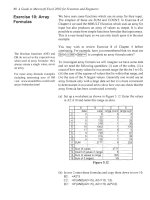
Exercise 8:
Functions
Array
When you use Help to get information about some functions you
may be told that they are
arrayfunctions.
Array functions generally
return more than one value. There are some important things to
remember when constructing a formula using an array function:
1.
When the formula generates more than one value,
you
must
select the output range before typing the formula.
2.
Once the formula is typed you complete it not with a simple
R

but with
(Ctrll+[Shift]+(Entercl].
When you do this, Excel
encloses the formula within braces
{
}
. You do not type these
braces.
3. If you need to edit an array formula you must select the entire
range of output values, edit the first entry and complete the
edit with
[Ctrl+(~Shift+[~].
In this exercise we will multiply
two
matrices with the MMULT
function to demonstrate
an
array function.
Do
not be concerned if
you are unfamiliar with linear algebra. We shall also see a shortcut
method to open the Insert Function dialog.
(a) Use InsertlWorksheet to add Sheet5 and drag the Sheet tab to
its correct place. Enter the labels shown in Al, A3, E3 and I3
as shown in Figure 4.13. The label in A3 was centred across
the three cells by selecting A3:C3 and clicking the
Merge
and
Center
tool. Enter the values shown in A3:G6.

Figure
4.13
70
A
Guide
to
Microsoft
Excel
2002
for
Scientists and Engineers
SQRT
Some Other
Mat hemat
i
ca
I
Functions
Returns the square root of a value; the
argument must be positive.
=SQRT(9) returns
3.
(b) Select I3:K6 and type
=MMULT.
Use
@m
to bring up the
Insert Function dialog. Enter A4:C6 as the first argument and
E4:G6 as the second. Complete the entry with
ICtrl]+[C>Shift+[Enterel].

GCD:
(c) Observe that with I4 as the active cell, the formula bar shows
(=MMULT(A4:CS,E4:GS)). Microsoft Excel has added the
braces,
(
},
to indicate an array function; the user should never
type these braces.
Returns the greatest common divisor.
=GCD(9,
18,
24)
returns 3.
(d) Save the workbook.
LCM'
The table below lists some other useful functions which are not
covered by the exercises. The examples are shown with constant
arguments only for clarity but they are more generally used with
cell references
or
expressions. Functions marked with
$
are
available only when the Analysis ToolPak is installed.
Returns the largest common multiple.
=LCM(S,
18,24)
returns
72.
QUOTIENT'

Returns the integer portion of a division.
QUOTIENT(28,
9)
returns 3.
FACT
Returns the factorial of a number.
FACT(4) returns 24.
RANDBETWEEN'
RAND
inserted, type
=RAND()
then press
=RANDBETWEEN(a,b)
is
equivalent to
RAND()*(b-a)+a.
not
-
[Entercl]
.
Using
Functions
71
MDETERM
M
INVERSE
MMULT
These return the matrix determinant of an
array, the inverse of a matrix, and the product
of

two
matrices, respectively. These are used
in
Chapter
10.
Working
with
Time
At the end of the last chapter brief mention was made of how
Microsoft Excel deals with dates and time.
You
may wish to have
a time value (for example, the value
85)
displayed
in
the form
1
:25
to denote
1
hour and 25 minutes
or
1
minute and 25 seconds. To
achieve this you must first convert the value to
a
fraction of a day
and then give it a custom format.
This

is
demonstrated in Figure
4.14.
Row
1
contains a series
of
values. The formula in C2 is
=CI-BI
and is copied to
JI.
The
formula
in
B3
converts the number of minutes
in
B
1
to days with
=B1/(24*60).
This also is copied to column
J
after giving it the
custom format
h:mm.
C2 computed a time difference with
=C3
-
83

and
is
similarly formatted. The equivalent quantity is computed
in
row
5.
C5 contains the formula
=(C3
-
B3
)*(24*60)
where the
factor 24*60 converts days back to minutes.
Figure
4.14
72
A
Guide to Microsoft Excel 2002for Scientists and Engineers
Problems
1
.*
You are constructing a worksheet to compute the
number
of
rolls
of
wallpaper needed to cover a wall. You have a cell
called
Length
and another called

Height.
Give the formula
needed to compute the number of rolls to be purchased
assuming one roll covers
2.25
m2.
2.
The values in the range
A3:A53
ofyour worksheet are between
0
and 100. You need to know how many
of
these cells have
values of at least
50.
Use Help or the Function Wizard and find
how to use the
COUNTIF
function.
3.* You have selected the cell F3 and entered the formula
=MINVERSE(A3:D6)
to
get the inverse of the matrix stored
in
A3:D6. However, you get only one number. What went
wrong?
4.*
With
two

cells named
hypot
and
opp
holding values
representing
two
sides
of
a triangle what formula will return
the value of the angle
in
degrees?
5.*
The number of ways of permutating
n
distinct objects taken
Y
at a time
is
given by
n!
(n-r)!
P=
Assuming that
n
is
stored
in
AI0

and
Y
in
BIO,
give the
formula required to compute
P.
You
will
find one method
in
this chapter; the other may be found using Help.
Decision Functions
Concepts
The functions introduced
in
this chapter are useful when making
decisions. They include the IF function, the logical functions
AND,
OR
and
NOT
which enable one to make compound tests, and
functions such
as
VLOOKUP,
INDEX and MATCH that
look
up
values from tables in the worksheet. We shall also explore the use

of SUMIF and COUNTIF. Some array formulas are explored.
The
IF
and the
The 1F function
is
used when you want
a
formula to return
different results depending on the value
of
a
condition.
As a simple
example, suppose A2:A21 contains the grades of
20
students and
you wish to have the word ‘Pass’
or
‘Fail’ in the
B
column
depending on whether the student’s grade is
50
or
greater. The
formula
=IF(A2>=50,
“Pass”,
“Fail”)

is
typed into B2 and copied to
B2:B21. Figure
5.1
shows the
syntax
for an
IF
function formula.
Functions
Equal sign to begin the formula
Condition to
be
tested
function name
=IF(condition, true-value, falsevalue)
Value
to
return
if
condition
is
true
1
Value
to
return
if
condition is false
Figure

5.1
A
condition
has the
form:
Expression-
1
Comparison Operator Expression-2
Expression-
1
and Expression-2 are any valid Excel expressions
composed
of
cell references, constants and functions. Essentially,
an expression
is
a
formula without the equal sign. Thus to test if
cell A3 has
a
value
of
5
the condition
is:
A3
=
5.
Here the first
expression

is
a simple cell reference, while the second one
is
a
constant. An example
of
a more complicated condition would be:
(AI+A2)*10
>
Bl/B2.
74
A
Guide to Microsoft Excel
2002
for Scientists and Engineers
The comparison operators are:
equal to
greater than or equal to
less than or equal to
-
-
>
greater than
>=
<
less than
<=
0
not equal to.
Some examples of IF formulas:

(a)
=I
F(
A2<0,
“Negative”, “Positive”)
Returns the text ‘Negative’ if A2 has a value less than
0,
otherwise it returns ‘Positive’.
(b)
=IF(AIO-BIO
<=
0.001,0,1)
Returns
0
if (A10-B10) is less than or equal to 0.001,
otherwise it returns
1.
(c)
=IF(ABS(AIO-BIO)<=EPSILON,
A10, B10)
The value in A10 is returned when the absolute value
of
(A10-B10) is less than or equal to the value stored in a cell
called EPSILON, otherwise the value in
B
10 is returned.
(d)
=IF(SUM(A12:A20)>0, SUM(A12:A20), “Error”)
If the sum of the range is greater than
0,

that value is returned,
otherwise the text ‘Error’ is displayed.
(e)
=IF(D2<0, NA(), D2)
When D2 is negative, the function NA() causes the Excel value
#N/A (meaning ‘not available’ or ‘not applicable’) to be
displayed. Sometimes we use this to mean ‘Display something
is wrong’.
(f)
=IF(Al, “True”, “False”)
This will return the textual value ‘True’ if
A1
contains a non-
zero value, a formula giving a non-zero value, or the TRUE
value. If A1 is empty, has the value
0,
or the FALSE value then
the text ‘False’ is returned.
IF functions may be
nested.
This means that within one IF
function, we may use another
IF
function for either or both
returned values.
Decision Functions
75
corner
of
the

cell
(a)
=IF(A1>10, IF(A1>50, “Big”, “Medium”), “Small”)
It is clear that if the condition A
1
>
10
is false then the first IF
returns ‘Small’. What happens if the condition is true? The
second IF comes into play. When A1
>
100,
the inner IF returns
‘Big’, otherwise it returns ‘Medium’.
A B
C
A B
C
12 =4/2
4 12
2
4
2 =AI=BI =CI>BI
=CI<=BI 2
TRUE
TRUE
FALSE
3
=5*A2
=5*B2

=5*C2
35
5
0
(b)
=IF(AI
>IO,
IF(A1>50, “Big”, “Medium”), IF(A1
<O,
“Negative”,
“
Sm a
I I”))
Here both the true-value and the false-value of the outer IF are
themselves IF functions.
Nesting up to seven levels is permitted provided the total number
of characters in the cell does not exceed 1024. Remember you may
use spaces in the formula to make it more readable.
A formula may be constructed using just a condition. Such
formulas will return the Boolean values TRUE and FALSE. Some
simple examples are shown in Figure
5.2
in which the left-hand
side displays the formulas while the right-hand side displays the
values. Row
3
demonstrates that TRUE and FALSE values are
numerically equivalent to
1
and

0,
respectively.
(a)
=IF(AND(A2>0, A24 I),
A2,
NA())
The value A2 is returned if A2 is greater than
0
and less than
1
1.
Otherwise, the function NA() returns the error value #N/A.
76
A
Guide
to
Microsoft
Excel
2002
for
Scientists and Engineers
14
15
(b)
=IF(OR(A2>0,
62>A2/2),
3,6)
Returns the value
of
3

if either A2
>
0
or
B2
>
A2/2. If neither
condition
is
true, the value
6
is
returned.
J
1.24
0.36
0
1
0
1.05 0.55
0
0
0
(c)
=IF(NOT(A2=0), TRUE,
FALSE)
This is the same as IF(A2=O, FALSE, TRUE).
(d)
=IF(NOT(OR(AI=I, A2=1)), 1,O)
This is a somewhat contrived example. It returns

1
if
both A1
and A2 have a value that is not
1.
Exercise
1
:
A
What-if
Acme Inc. makes widgets which are tested before being sold. The
testing gives
two
values,
P
and
Q.
The requirements are that
P
be
at least 1.25 and
Q
be no more than
0.5.
Using some sample data,
Acme wishes to know how many widgets pass the tests and how
the results would change
if
the specifications were to be altered
slightly.

For
this exercise, we will use only 10 data sets but in a
real
case
there might be hundreds. The results of this small sample
of widgets are shown in Figure 5.3.
Analysis
pmin
qmax
0.5
A
Figure
5.3
(a)
Start a new workbook. On Sheet1 enter the text and values in
Al:E5. Name the cells C2 and C3 as
pmin
and
qmax,
respectively. Enter the numeric values in A6:B
15.
Decision
Functions
77
L
3
4
(b) Enter these formulas:
C6:
=IF(AG>=pmin,

1,
0)
D6:
=IF(BG<=qmax,
1,O)
E6:
=IF(AND(AG>=pmin,BG<=qmax),
1,
0)
Resistors
10
20
35
40
50
50
1/R
0.1
0.05
0.028571
0.025 0.02
0.02
Each of these formulas returns a value of
1
if a condition
is
met, otherwise they return
0.
The first tests the
P

value, the
second tests the
Q
value, and the third tests both values.
(c) Copy the three formulas down to row 15.
(d) Enter the text
in
B16
and
right align it.
(e)
InC16entertheformula=SUM(C6:C15)/COUNT(C6:C15)and
copy it to the
two
cells to the right.
(f)
We are now ready to play the what-if game. By changing the
value in C2, we can get answers to questions such as ‘What
percentage of widgets would pass if the acceptable value of
P
was (i) raised to 1.3
or
(ii) lowered to 0.22?’
(g) Save the workbook
as
CHAP5.XLS.
Exercise
2:
Avoiding
In Exercise

7
of Chapter 2 we developed a worksheet to find the
effective value
of
four resistors in parallel. It was noted that we
could not use the worksheet
for
less than four resistors
by
using a
zero value since we would run into the divide by zero problem. On
Sheet2
of
CHAP5.XLS we will develop a worksheet to compute
the effective value of up to six resistors
in
parallel using the
formula
1/R
=
CUR,. Our final product will resemble Figure 5.4.
Division
by
Zero
IAI BI
CI
DI
El
FI
G

1 IResistors
in
Parallel
I
nl
I
I
I
I
I
I
(a) Enter the text shown in column A. In A5 type
Re
and
in
the
formula bar select the letter
e
before using the command
FgmatlCells and selecting
Subscript
on the Font tab. Enter the
numeric values shown in
B3:G3.
78
A
Guide
to
Microsoft Excel
2002

for Scientists and Engineers
1
2
3
4
Exercise
3:
Quadratic
Equation Solver
Quadratic Equation Solver
a
b
C
disc
1
5
6
1
(b) The formula in B4 is
=IF(B3>0, 1/83,
"
"
) which returns the
reciprocal of the resistance if its value is greater than
0.
Otherwise, the formula returns a space. Copy this across to G4.
61
Root
1
I

-2
(c) In B5 enter
=I/SUM(B4:G4).
Check the result using pencil and
paper.
(OK,
you can use your calculator!)
Root
21
-3
(d) Now let us see if it works for four resistors. Enter 25 for the
value of the first four resistors and either leave the last
two
empty or use the value
0.
Do
you get 6.25 ohms? Save your
workbook.
It was noted in Chapter 4 that the SUM function can tolerate non-
numeric values in cells forming part of an argument. We would be
in trouble if we did not know the
SUM
function and, in its place,
used
=B4
+
C4
+
D4
+

E4
+
F4
+
G4.
The simple formula will not
tolerate non-numeric values and will return the #VALUE! error.
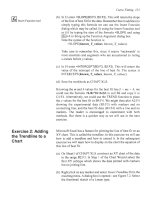
In this exercise we design a worksheet to solve a quadratic
equation in the form
ax2
+
bx
+
c
=
0
using the quadratic formula:
-b
k
Jb2
-
4ac
2a
X=
The quantity
JG
is called the discriminant because its value
determines the number
(0,
1

or 2) of real roots of the equation.
When this exercise is completed, the worksheet will resemble that
in Figure 5.5.
I
I
A
I
B
I
C
I
D
I
E
I
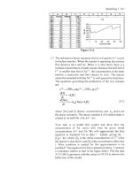
(a) Open CHAP5.XLS. On Sheet3 enter the values shown in
A1 :C3. Select A2:C3 and centre the entries with the button on
the Formatting toolbar.
Decision Functions
79
Disc
>
0
Disc
=
(b) With A2C3 still selected use the command lnsertlNamelCreate
to give the cells A3:C3 the names in the cells above them.
A
I
B

C
D
5
Number
of
real roots
2
6
Root
1
I
-2
Root
2
-3
A
B
C
D
5
Number
of
re!!, roots
1
6
Double
Root]
2
(c) Type
disc

(short for discriminant)
in
E2.
In
E3 enter the
formula
=b*b
-
4*a*c-
in E3. Centre E3:E4 and create the
name
disc
for the cell E3.
Disc
<
(d) Temporarily ignore the entries
in
A5, B5, A6 and C6 of Figure
5.5. Type these formulas
in
B6 and D6:
B6:
=(
-
b
+
SQRT(disc) )/(2*a)
D6:
=(-b
-

SQRT(disc)
)/(2*a)
A
B
C
D
’
5
Number
of
reg1
roots
0
I2
(e) Save the workbook CHAP5.XLS.
You
now have an operational worksheet. Test it with quadratic
equations whose roots you know. What happens if the value of the
discriminant is negative? Cells B6 and D6 show the error value
#NUM!
since it is impossible to evaluate the square root of a
negative number without entering the realm
of
imaginary numbers.
The next steps will improve the behaviour of the worksheet when
the discriminant
is
negative and add some additional information.
The results we are aiming for are shown
in

Figure 5.6.
Figure
5.6
(f)
Enter the text in A5.
In
C5 enter the formula
=IF(disc<O,
0,
IF(disc=O,
1,
2)).
This returns
0
when the discriminant
is
negative,
1
when it
is
zero and
2
in
all other cases.
(g)
In
A6 enter the formula
=IF(C5>O,IF(C5=1,
“Double
Root”,

“Root
I”),
“
’I).
If there
is
one root, this returns the text ‘Double
Root’, if there are
two
identical roots it returns ‘Root
1
’.
When
there are no
real
roots, it returns an empty test string.