A Guide to Microsofl Excel 2002 for Scientists and Engineers phần 2 pptx

22
A
Guide to Microsoft Excel
2002
for Scientists
and
Engineers
Exercise
3:
Formatting
Resu
I
ts
Our project is almost complete.
All
that remains is to change the
way the results are displayed. For this project it is inappropriate to
display
so
many digits after the decimal; we need integer values.
(a) Select range B4:B13 on the worksheet of the previous
exercise. From the Format command on the menu select
Cells.
In the resulting dialog box select the Number tab
-
see Figure
2.5. The General format will be highlighted in the Category
box. This is the default number format. In most cases, an entry
in a cell having the General format is displayed the same way
as it was typed. When the cell
is

not wide enough to show the
entire number, the General format rounds numbers with
decimals and uses scientific notation for very large and small
numbers
.
the
(b) In the Category box, click the Number tab. Change the value
in the Decimal places box to
0.
You may use the spinner
or
type the value in the box. Click the
OK
button to close the
dialog box. Your worksheet now displays integer values.
Figure
2.5
(c) There is another way to do this. Click the Undo button on the
The
Undo
tool
Standard toolbar to display the original values.
(d) Select B4:B 15 and click once on the Increase Decimals button:
Basic
Operations
23
pJ
The Increase Decimals
tool
b"gl

The Decrease Decimals
tool
if you try to use the Decrease Decimals tool Excel will make
a ping sound to warn you this is impossible
-
B4
has an integer
value
so
it cannot be made to display any fewer decimal
places.
All
the numbers now display one decimal place. Click
the Decrease Decimals button once to display them all as
integers.
It
is
important to know that formatting changes only the way
a value is displayed. It does not change the actual value stored
in
a cell. We look at this
in
Exercise
4.
(e) Save the workbook
CHAP2.XLS.
Notes on Precision
Numbers are
stored
with 15-digit precision by Microsoft Excel.

The number of digits
displayed
depends on the format and width
of the cell. If the user has not applied a format, Excel uses the
General format.
A
cell may be formatted to display a required
number of decimal places or to use scientific notation. We do this
with the command Fo-mat(Cgll(Number or by using the Increase
and Decrease Decimals button.
and Formatting
In
the next exercise we demonstrate that formatting does not alter
the stored value. Later we will examine functions that round values
to a specified number of decimal places. You should also be aware
that when
a
cell
is
copied or moved, the target cell gets the same
format as the source cell.
Excel can store positive numbers as large as
9.99 999 999 999
999
x
and as small as
1
x
10-'07.
The range for negative

values is
-
9.99 999 999 999 999
x
1
0+307
to
-1
x
1
O-307.
The range
of values in Microsoft Excel
is
thus while a typical hand
calculator has
a
range of
1
O*99.
You should be aware that conversion from decimal to binary can
result in round-off errors. Suppose you perform
two
complex
calculations and expect
A99
and
B99
to have the same values.
Because of round-off errors, the

two
values may differ by a small
amount and the formula
=A99
-
699
may not give exactly zero but
a value such as
0.000
000
000
000
008
or
8E-15.
Just as
in
decimal
notation (base
10)
the result for
10/3
cannot be written with infinite
precision as a real number,
so
in binary (base
2)
there are some real
numbers that cannot be represented exactly.
24

A
Guide to Microsoft Excel
2002
for
Scientists
and
Engineers
A
I
B
I
C
I
Displayed and stored values
Enter the values 27.05 and 26.1
in
A1 and A2 of an empty
worksheet. In A3 enter
=AI
-
A2
and the value
0.95
is
displayed as
expected. Now we look at the actual value stored for
A3.
Progressively increase the number of displayed decimal digits by
clicking the appropriate button on the Formatting toolbar. After a
while the value 0.94999

is
displayed. Clearly there has been
round-off error since the result should be
0.95
exactly.
Programmers seldom test if two numbers are exactly equal but
rather they test if the absolute difference
in
the two numbers is less
than some arbitrarily small quantity.
D
E
Exercise
4:
Displayed
The purpose of this exercise is to demonstrate that formatting
changes only the way
in
which a value is
displayed.
The
stored
value
is
unaltered. When completed the worksheet will resemble
that
in
Figure 2.6.
and

Stored Values
2
1 1
Figure
2.6
(a)
Open the workbook CHAP2.XLS and click on the Sheet2 tab
to begin a new worksheet. Begin by typing the text
in
A
1
:C3.
Entering the text in B3:C3 presents a small problem. The equal
sign alerts Excel to use a formula but this
is
not what we want.
Before typing the equal sign, type a single quote (an
apostrophe) to tell Excel that you want text.
(b) In row
4
enter the following:
A4: the value 1.234.
B4: the formula =A4
C4: the formula =A4+2
D4:
the formula
=A4*2
(c) Using the Decimal tools, format A4 to display one decimal
place. The cells
A4:D4

should show the same values as
in
Figure 2.6.
Basic
Operations
25
(d) Make
A4
the active cell. The value displayed in
A4
is
1.2
but
from the formula bar we see that the stored value is
1.234.
Unfortunately, one cannot see the applied format by looking
here. You may check how a cell
is
formatted by selecting the
cell and using the FgmatlCglllNumber command.
If we wish to have a value stored with a set number of decimal
digits, we use the
ROUND
function which is discussed in a later
chapter. It
is
possible to use the IoolslQption command to have
Excel use the same precision as the displayed value. This may be
useful
in

financial worksheets but is not recommended.
In the next part
of the exercise we see
an
oddity of Microsoft
Excel. When a formula is typed into a cell which has not been
previously formatted (Le. it
has
the General format) and the
formula contains only (i) references to one or more cells with
identical formats and (ii) either no operator, or only the addition or
subtraction operator, then the cell with the formula gets the format
of the referenced cells.
(e) Type the text in A6.
(f)
Enter the value
1.234
in
A7
and format it to one decimal place.
(g)
In
B7
enter the formula
=A7.
The value
1.2
is
displayed. Cell
B7

has taken on the format
of
A7
because the formula
is
a
simple reference to a formatted cell. We may format the cell to
restore the value of
1.234
if that
is
required.
(h)
In
C7
enter
=A7+2.
Again the value is displayed with one
decimal place. However, when
=A7*2
is entered in
D4
we get
2.468
-this cell does not take on the format of
A7.
If you use
a formula such
as
=B7+C7

in
D7,
the result
will
be displayed
with one decimal place since that is how
B7
and
C7
are now
formatted.
(i) Save the workbook.
Exercise
5:
Formats
In
this exercise we see that with the Copy and Paste commands
both the values and the formats are copied. However, Excel
2002
provides a way to avoid copying formats. The worksheet will
resemble Figure
2.7
when the exercise
is
complete.
Get
Copied
26
A
Guide to Microsoft Excel

2002 for
Scientists and Engineers
(a) On Sheet3
of
CHAP2.XLS, type the text shown in Al:A5.
Type
12.555
in B3 and copy this to C3:E3 by dragging the
fill
handle to the right.
UvLLLIIIUIIYa
v1
$*XU
LV"l.7
"11
I
Standard toolbar. But there are
t7
more ways;
you
may find one
them more convenient
Paste action we could use the menu
Pnmm-mAo
nv
the
tnnla
nn
the
XO

of
Keyboard shortc
[Ctrll+C
and
for
Paste use
[Ctrl/
(b) Format cells in B3:E3 to display the values as in Figure 2.7.
(c) Select B3:E3 and click the Copy tool. Make B5 the active cell
and click the Paste tool. Note that the values in the destination
cells are displayed with the same formatting as the source
cells.
The Copy operation places material on the Clipboard. To warn
you that this has occurred, an animated border (the 'ant track')
is placed around the copied material. While the ant track is
present you can paste the material on the same worksheet; on
another worksheet in the same or another workbook, or in any
open Windows document. When you perform any other action
in
Excel, the material is removed for the Clipboard and the ant
track goes way. This
is
a safety precaution not used in other
applications; numeric material erroneously pasted into a
worksheet might not be spotted and could lead to incorrect
business decisions.
(d) Excel
2002
has a new feature associated with the Paste
operation: a Paste option smart tag appears. It resembles the

Paste icon on the toolbar but when the mouse hovers near it a
down arrow is added to the icon. Click the icon to open the
smart tag. It offers options to use the formatting from the
New Excel
2002
feature
Basic
Operations
27
source or to match the formatting
of
the destination. Use Help
to learn about the other options when you know more about
Excel. Save the workbook.
Exercise 6:
Too
Many
In this exercise we discover what to do when the value in a cell has
too many digits to display. There are a variety
of
ways to change
the column width to accommodate the value.
Digits
(a) When we opened the worksheet that was to become
CHAP2.XLS it very likely had three worksheets since this is
the default setting. We need a new worksheet for this exercise.
Use the command InsertlWorksheet to make a new one. Now
look at the sheet tabs and locate the tab for Sheet4. It was
placed to the left
of

whichever was the current sheet when you
use the insert command. Clearly it is in the wrong place. Click
on the Sheet4 tab and drag it to the right
of the Sheet3 tab to
locate it correctly.
(b) Enter the value
123.456
in Al.
(c) Using the Increase Decimal icon, increase the number
of
decimal digits. After a few clicks the value has filled the cell
and Microsoft Excel automatically widens the cell to keep pace
with the number of characters displayed. There is, however, a
limit; a cell cannot hold more that 256 characters. Furthermore,
do not be misled by all those zeros! Microsoft Excel stores
numbers to a precision of 15 digits. Adjust the value to about
8
decimal places.
(d) Place the cursor in the column headings and position it on the
divider between the
A and
B
headings. The cursor will change
to a new shape
-
see Figure 2.8. Drag the column divider to the
left making column
A
narrower. The cell now displays
##########

indicating that the cell is not wide enough to
display the value with its current format.
Figure
2.9
(e) In the last step we changed the width
of
a column but we have
28
A
Guide to Microsoft Excel
2002
for Scientists and Engineers
Shortcut:
You
can also open the
Format dialog box
fi-om
the
popup
menu
that
appears
when
you
right
click
in
a
cell.
Shortcut:

To
change
a
column
width
to accommodate the widest
entry
in
that column, double
click
on the
divider
to
the
right
of
the
column header.
Exercise
7:
Ca
I
cu lat
i
o
n
Example
no idea what the actual width is. This time we will change the
width to a specified size. With A1 as the active cell, use the
command Fo-rmatlColumnlWidth. In the Column Width dialog

box (see Figure 2.9) enter the value 8.43. This is the default
column width with Aria1 font of size
10
or
11
points and is
large enough to display eight digits.
(f)
The cell may still display
#######.
Use Format(Cgl1 to display
the value with
3
decimal places. It should now
fit
the column.
(g) In
A2
enter the value
12345678912.
This time Excel does not
expand the column to accommodate all the digits because the
column has been given a fixed width. Rather, Excel displays
the value in scientific format as 1.23E+10 which is to be
interpreted as 1.23
x
10".
Microsoft Excel behaves differently with text entries. If you type
a text entry with more characters than the cell can hold, the entry
will overflow into the cells to the right provided they are empty.

(h) Type Sample heading, in B
1.
Both words are readable but
much of the second overflows into column C. Now type
Another heading
in C1. Most of the characters
of
the second
word in B
1
are now lost. B
1
is not wide enough to display its
contents and text overflow is not permitted now that C1 is
occupied.
(i) We now experiment with another way of widening a column.
With B1 and C1 selected, use the command FormatlColumnl
-
AutoFit Selection. The
two
columns are made exactly wide
enough for B
1
and C
1
to hold their contents.
The AutoFit command may be used with any type of data, numeric
or textual. If we select the column headings rather than a range, the
AutoFit command makes the columns the correct width for the cell
in each column with the greatest need for space.

(i)
Save the workbook.
Once a worksheet has been set up to solve a problem, it may be
used repeatedly for the same type of problem but with different
input values. For example, if you had one quadratic equation to
solve, it might not be worth the effort to design a worksheet to do
it. If you had a dozen or
so
equations to solve, then a worksheet
Basic Operations
29
solution would be more efficient than using a pocket calculator.
Other advantages of the worksheet are (i) the ability to see what
values you have used and (ii) the facility to modify the calculation
without re-entering all the data.
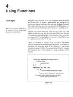
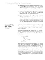
In this exercise we will design a worksheet to compute the
effective resistance of four resistors in parallel. The four resistors
(RI,
R2,
R3
and
R4)
in Figure 2.10 have the equivalent resistance
value of the single resistor
(Re)
whose value is determined by the
relationship shown in the figure.
3
Resistors
1IR

25 0.04
0.406667
2.459016
I12
IRe
I
2
4590161
R1
R4
Re
11111
Re
RI
R2 R3
R4
-
-=-+-+-+-
Figure
2.10
(a) Using the method in the last exercise, insert Sheet5 in the
correct position on the workbook CHAP2.XLS.
(b) Enter only the text and values shown in A1 :A1
0
and B
1
:B3
of
Figure 2.10.
(c) In B4 enter the formula

=1/A4.
Copy this formula to B5:B7 by
either dragging the
fill
handle of €34
or
double clicking on B4's
fill
handle.
handle
of
I34
causes the formula t
be copied down the table.
(d) The formula in B9 is
=B4+B5+B6+B7,
giving the value 1/Re.
Remember you may add spaces around the addition operators
if you wish. Later we shall use a function to evaluate a
summation like this.
(e) The formula in B10 is
=1/B9
to give the value of Re.
(f)
Test your worksheet with the values 2,2,4,4. Since 1/Re will
be
%
+
'h
+

%
+
%
or
1%,
your worksheet should give Re as
0.666667.
Whenever possible, check a new worksheet with a
30
A
Guide to Microsoft Excel 2002 for Scientists and Engineers
Exercise
8:
Entering
Formulas
by
Pointing
few manual (or mental) calculations. Save the workbook.
While our worksheet is able to compute the equivalent resistance
of any four resistors
in
parallel, it cannot be used for fewer. If we
enter
0
in A7 (for example), Excel will return the error value
#DIV/O!
in
B7.
The same error value will be displayed for all
formulas that use B7. Incorporating an

IF
function (see Chapter
5)
in
the formulas used
in
B4:B7 would make the worksheet much
more versatile.
What we did in A4:B
10 is similar to how we would manually solve
this problem with paper, pencil and calculator, writing down every
intermediate result rather than using the calculator’s memory.
Wherever there is repetition (e.g. calculating the reciprocals
in
this
example), the worksheet method simply requires us to copy
formulas. These
two
points may help you design your own
worksheets.
In
this exercise we look at an alternative method to typing cell
references when building a formula. When you type
a
cell
reference you must take care to use the correct address. With
larger, more complex worksheets, it
is
easy to make a mistake. The
alternative method

is
to point to the cell with the mouse. It is akin
to saying ‘use that one’.
For the problem in Exercise 7, clearly we could combine steps (d)
and (e) and compute the value of the effective resistence
in
one
formula:
=
1/(
B4+B5+B6+B7). The parentheses are essential.
(a) In A12 enter the text
Re.
(b) In
B
12, begin the formula by typing
=1
I(.
Now left click on cell
B4 and observe the result
in
the formula bar
-
the formula is
now
=l/(
B4. Type the plus sign and click
on
B5. Continue until
the formula reads =1/(84+85+B6+87 and click on the green

check mark
in
the formula bar.
(c) If you have entered everything correctly, Microsoft Excel
politely points out that there
is
a small error and offers to
correct it by adding the closing parenthesis. Click the Yes
button of the dialog box.
(d) Double click on B12 and note the status bar now reads
Edit
rather than
Ready.
But the more obvious change
is
the
Range
Basic Operations
31
Finder
feature which causes the cells and ranges to which the
formula refers to be displayed in colours, and matching colour
borders to be applied to the cells and ranges referenced in the
formula. This provides a convenient graphical way for us to
check formulas. Save the workbook.
Exercise
9:
In Exercise
2
we saw that Excel normally treats cell references as

relative references when a formula is copied. There are times when
References:
Relative’
this is not what we need. If the formula refers to the cell A1 we
Absolute and Mixed may modify the reference by adding one or more
$
symbols.
Reference Result when formula is copied
=A1
the row and the column may change
=A$1
the row remains constant, the column may change
=$A1
the column remains constant, the row may change
=$A$l
both the row and the column remain constant
A cell reference in the form A1 is called a
relative
reference while
$A$1 is called an
absolute
reference. The forms $A1 and A$1 are
mixed
references. Remember that when a formula is copied to the
same row, the row reference is unchanged without the need for the
$ symbol. Similarly, when a formula is copied to the same column,
the column reference is unchanged without the
$ symbol.
To demonstrate the use of mixed references, we will develop a
simple worksheet that displays a multiplication table as shown in

Figure 2.1
1.
Shortcut:
To enter a series
of
IAI
BlCl
DI
El
FIG1
HI
I
I
J
11
I
21
31
41
51
61
71
SI
91
10
Figure
2.11
(a) Insert Sheet6 in the workbook
CHAP2.XLS.
Start by entering

the values
2
and
3
in
B
1
and
C
1.
Use the Series Fill method to
complete the row. Enter the data in column
A
in a similar
manner.
32
A
Guide to Microsoft Excel
2002
for Scientists
and
Engineers
Exercise
IO:
Editing
and Formatting
Note:
We
could,
of

course, use the
equivalent formula:
=(
B4
*
B8)/(A9
-
E4)- D4/(A9/'2).
(b) In B2 we need a formula to compute A2
x
B
1.
If we use
=A2*B1
we will not be able to copy it. What we need is
=$A2*B$l.
The
$
before the
A
in the first term ensures that,
when the formula is copied across the worksheet, the reference
will always be to that column. Similarly, the
$
in the second
term keeps the reference to row
1
constant when the formula
is copied down the worksheet.
The

$
signs may be typed as you enter the formula but we shall
use another technique. Type
=A2
to start the formula. Now
press
[F4)
repeatedly until the formula reads
=$A2.
Next add
*B1
to the formula and again use
IF4]
to make the formula read
=$A2*B$l.
(c) Copy B2 to B2:JlO.
(d) Examine the values and the formulas in a few cells to make
sure you understand the process.
(e) Save the workbook.
In this exercise we construct a table to display the pressure of a gas
at various temperatures and volumes using the van der Waals
equation:
RT
a
p=
V-b V2
We would like to be able to change the values of
a
and
b

so
that
our table may be used with different gases,
so
we will place these
values in their own cells rather than
in
the formulas. We will also
place the value of the gas constant
R
in a cell to provide
documentation
-
and to allow us to change it quickly if we use the
wrong value. The final worksheet will resemble that in Figure 2.12.
Do
not worry about the negative pressure value
-
the gas has
condensed under these conditions and the equation is not really
applicable.
(a) Open the workbook CHAP2.XLS and move to Sheet7. Type
the text shown
in
rows
1
to
7
of
Figure 2.12.

In
C4 type
C02.
Enter the values
in
B4:E4. We will format the cells (centring,
subscript, etc.) later.
Basic
Operations
33
(b)
Enter the values in
B8:H8
and
in
A9:A
method.
8
using the Series
Fill
(c)
In
B9
enter the formula
=(B4*B8)/(A9 E4)-D4/(A9*A9).
The
pointing method from Exercise
8
would be appropriate here.
Click the check mark

in
the formula bar when the formula is
complete. The cell should show the value
1374.21.
Correct the
formula if needed. Examine the formula making sure you
understand how it computes the pressure for
V=
0.05
litres and
T=
250
K.
Figure
2.12
We need to modify the formula
in
B9
before copying
it
to the range
B9:H18.
There are three considerations: (i)
In
the formula,
B4
refers to the value of the gas constant,
D4
to the
a

constant and
E4
to the
b
constant. These references must not change when the
formula is copied; (ii) On the other hand
B8
refers to the
temperature and we have a range of these
in
row
8.
When the
B9
formula is copied, the reference to
B8
must still refer to row
8
but
the column must change; we need to replace
B8
by
B$8;
and (iii)
The references
to
A9
must continue to point to the volume values
in
column

A
but as the formula is copied the row must change.
So
we need to use
$A9.
In
summary, we need to edit the formula to read
=($B$4*B$8)/(A$9
-
$E$4)
-
$D$4/($A9*$A9).
We shall not retype the formula, rather
we shall edit the existing one. We shall
do
this
in
a series of steps
to illustrate the various options that are available.
34
A
Guide
to
Microsoft Excel
2002
for
Scientists
and
Engineers
HMerge and Center tool

-
Center
Align
tool
(d) Move to cell
B9
and enter editing mode by either double
clicking or by pressing
[.
(e) We have a variety of options for editing the formula.
In
cell
B9,
move the mouse pointer
in
front of the reference to
B4
and
click to position the insertion point. Type the
$
symbol. Move
the insertion point
in
front of the
$
in
B4
and type another
$
symbol. Now move the insertion point between the

B
and the
8
in
B8
and insert
a
$
symbol.
(f)
Next move the insertion point anywhere within the first
reference
to
A9
-you may have the insertion point
in
front of
the
A,
between the
A
and the
9,
or just after the
9.
Now press
[F41
repeatedly and watch the reference cycle through the
values
$A$4, A$4, $A4

and
A4.
Stop when you have the
required value of
$A9.
Use the same technique to change
E4
to
$E$4.
Click the green arrow in the formula bar to complete
the entry and return to ready mode.
(g) We have not completed the editing
so
we will re-enter the edit
mode and explore another way
of
editing. This time we will
activate the edit mode by pressing
m.
It has the same effect
as double clicking but some users find it more convenient. For
variety this time, rather than doing the editing
in
the cell we
will do it in the formula bar. We need to replace
D4
by
$D$4
and
A9*A9

by
A$9*A$9.
Use whichever method you prefer:
typing the
$
or using
m.
Click on the green arrow
in
the
formula bar when you have completed the task.
(h)
B9
should now read:
=($B$4*B$8)/($A9- $E$4)-
$D$4
/($A9*$A9).
Copy it to row
18
and column
H.
Check that your
values agree with those in the table. If they do not, you may
need to edit
B9
and recopy it.
(i) Now some formatting to improve the appearance
of
some cells.
(i) Format the range

B9:H18
to display two decimal places.
(ii) Select
AI:Hl
and centre the
van der Waals

text over
these cells using the Merge and Center button. Use the
second item
in
the Formatting toolbar to increase the size
of the font to
14.
Click the Bold button on the same
tool bar.
(iii) Select
B3:E4
and centre the entries with the Center button
on the Formatting toolbar.
(iv) Using the technique
in
(i), centre the text
in
A6
over
columns
A:H
and the text in
B7

over columns B:H.
Basic Operations
35
(v) In C4 we have
C02
but wish to have
CO,
with the ‘2’ as
a subscript. Select C4 and start the edit mode. Highlight
the
2
and, from the menu bar, select Foymat(Cel1.s. Using
the Effect portion in the resulting dialog box (lower left),
click on the Subscript box to place a
J
in it. Click the
OK
button.
(j)
We will do more with this worksheet later. Giving the
worksheet a name other than Sheet7 will help us locate it.
Right click the sheet’s tab, select Rename from the menu and
type the name
VanderWaals.
Save the workbook CHAP2.XLS.
Exercise
1
1
:
What’s

In
the exercises
so
far, we have constructed formulas that use other
cells’ values by using cell references. It
is
possible to give a cell,
or
a range of cells, a name. The advantages of this are twofold:(i)
it is easier to remember where a value
is
stored if the cell has a
name and (ii) names are always treated as absolute references.
in
a
Name?
In
this exercise we use names with one letter. This is not a
requirement, we may use a name such as Gasconstant. Note that
names are not case sensitive
so
GASCONSTANT and Gasconstant
are treated as the same name. When single letters are used, R and
C
are invalid since Excel uses these letters for other purposes.
Similarly, we may not use a name which could be a cell reference.
However, we may add an underscore to create names such as
R-,
c-,
XI,

etc.
(a) Open CHAP2.XLS and move to the VanderWaals worksheet.
Delete the range
B9:H 18.
(b) With the range B3:E4 selected use the command
InsertlBamelCreate. A dialog box similar to Figure
2.13
appears. Excel has detected text
in
the top row and values
in
the lower one,
so
it correctly assumes that you wish to apply
the names
in
the top row to the corresponding cells
in
the
lower row. Click
OK.
(c) Move to
I1
and use InsertlNamelPaste.
In
the resulting dialog
box (Figure
2.1
1)
click Paste List. This lets us check what

names have been assigned to what cells. Note that
B4
got the
name
R-
not R. Delete the list or press the Undo button.
(d)
In
cell
B9
type the formula
=(R-*B$8)/($A9
-
b)
-
a/(
$A9
*
$A9).
Check its value and copy it to
B9:HlS.
36
A
Guide to Microsoft Excel
2002
for Scientists
and
Engineers
(e) Save the worksheet.
A'

R
c
'
D
EIF
G'
van
der
Waals Equation
of
State
R
Gas
a
b
008206
C02
359
00427.
iI
I
Figure
2.13
We used a semi-automatic method to create names for some cells.
We may also select a single cell and use ZnsertlEamelDefine to
name a specific cell.
There are a number of ways
of
referencing a named cell (or range)
in a formula. To enter, for example,

R-
in a formula we may (i)
type the name
R-,
(ii) point to the corresponding cell with the
mouse, and (iii) use the command lnsertlN_amelPaste, and select the
required name and click the
OK
button or simply double click on
the required name.
We began this exercise by deleting the range
B9:HlS.
We did this
to show how to build a formula with names. Alternatively, after we
had created the cell names, we could have used the command
InsertlN_amelApply to replace cell references by cell names.
A named cell or range may be referenced in any sheet of the same
workbook. It
is
possible to use the same name for
two
cells (or
ranges) in different worksheets of the same workbook. Suppose a
cell in Sheet1 is named
Mass,
and a cell in Sheet2 has the same
name. A reference to
Mass
in Sheet
1

will automatically refer to the
Basic
Operations
37
cell in that worksheet. If, in Sheet2, you need to reference the
Mass
cell of the other sheet, you would use
SheetI!Muss.
If we move to
Sheet3, where no cells are named, what would a reference to
Mass
mean? Generally, it would refer to the cell in Sheet
1
since this was
first named. However, it would be safer to qual@ the name using
either
Sheetl!Mass
or
Sheet2!Mass
as required.
Exercise
12:
Custom
In
Exercise 3 we discovered how to format numbers. We may, for
example, arrange to have three decimal places displayed, or to use
scientific notation. Excel also permits the user to develop custom
formats.
To
demonstrate this we will format numbers so that the

exponent is always a multiple of three
-
the engineering notation.
Formats
Figure
2.14
(a) Open CHAP2.XLS and insert a new worksheet. You may need
to drag the sheet’s tab to the right and correctly locate it.
(b) Enter the text shown in A1 :B3 of Figure 2.14. Enter the values
shown
in
A3:A9. When you enter the large number in A9,
Excel will display it in scientific notation; change this to the
number format with
two
decimal places.
(c) In B3 enter
=A3
and copy this to C3 by dragging the
fill
handle
to the right.
(d) Select B3 and format it to scientific notation with
two
decimal
places. Copy B3 down to B9 by double clicking its
fill
handle.
(e) Select
C3

and open the Format dialog either by using the
command FormatlC& or by right clicking the cell and
selecting the Format Cells item in the popup menu.
38
A
Guide to Microsoft Excel
2002
for Scientists
and
Engineers
J
Figure
2.15
(f)
Open the Custom tab on the dialog
-
Figure
2.15.
Place the
cursor in the Type box and backspace out whatever is there
already. Do
NOT
use the Delete button on the dialog box to do
this.
Type in the custom format in this form:
##O.OOE+O;
-##O.OOE+O;
0.
A
custom format has three parts separated by

semicolons. The first part specifies the format for positive
values, the second for negative values, and the third for zero.
By limiting the number of digits before the decimal to three we
have forced Excel to use the engineering notation where the
exponent is a multiple of three. Unfortunately, the result is not
very pleasing for values less than 1000. We may display as
many digits after the decimal as we wish. If you wish not to
have zeros displayed use
I'
for the third part of the format.
(8) Double click on the fill handle
of
C3 to copy the formula down
to C9. Save the workbook.
Basic
Operations
39
Exercise
13
and
Such
,:
Symbols We may need to use symbols and Greek letters
in
table headings so
we need to know how to get such text as
Temp
OC
and
AV=x?Ah

into cells. The reader is encouraged to investigate these ways
of
obtaining such results.
(a) Certain symbols are readily generated by holding down the
key and entering a four-digit code on the number pad (it
must be the number pad, not the digits on the top row
of
the
'typewriter' keys). The first
two rows of Figure
2.16
show
some useful symbols. Thus
(Anl+O
I
77 gives
f,
the plus-minus
symbol.
This table is most easily made by entering the numbers
in
the
second row, typing the formula
=CHAR(A2)
in
A3
and copying
it across the row.
So
we may have a cell display

"C
either by
typing
mAt0186
followed by C, or with the formula
=CHAR(186)&"C".
The former is,
of
course, more convenient.
Note that we can use this method to get superscripts
in
text (as,
for example,
R2
and
m3)
but we can
also
get these by
formatting a normal digit
as superscript
-
see step (i) of
Exercise
10.
~~~
Figure
2.16
(b) Greek letters are obtained with the Symbol font. Suppose you
want a cell

to
display
AV.
Begin by entering the two letters
DV. Now either select the D in the formula bar, or double click
the cell to enter edit mode and select the D
in
the cell. Next
change the font
of
the selected letter. This may be done with
the command Fgmat(Cg1ls and opening the Font tab. But it
is
more convenient to use the Font box on the Formatting toolbar.
Remember that there
is
no need to scroll down the list, typing
40
A
Guide to Microsoft Excel
2002
for Scientists and Engineers
S
will jump to the first font beginning with this letter.
The formula bar does not display the formatted value. When
you select a cell having some or all the characters formatted in
Symbol font, you will see Roman (regular) characters in the
formula bar generally
in
Aria1 font.

New
Excel
2002
feature
(c) If you are familiar with Word you will know that one can use
InsertlSymbol to get symbols and Greek characters into a
document. Until the latest version, Excel did not support this
feature. However, one could use the Windows procedure
(StartlProgramsIAccessories)Character
Map) to copy symbols
to the clipboard for pasting into a cell. With Excel 2002 one
has access to the InsertlSymbol dialog. Indeed, it is a much
improved feature
-
see Figure 2.17.
Exercise
14:
Fractions
Figure
2.17
From Figures 2.16 and 2.17 we can see that it is possible to enter
fraction symbols into cells. It is important to realize that fractions
entered in either of these ways are just symbols. They are not
numerical values and cannot be used in mathematical operations.
Functional fractions are possible. A cell can display, for example,
2 1/4 but its stored value is, of course,
2.25
-the display results
from formatting.
Basic Operations

41
3
4
If you mistakenly type
1/8
in
A4,
3.5 2
7
Total
28
Excel
Will
assume
you
want
(I
August or
8
January dep
on your regional settings).
the entry and use EditlClearlEo
to remove the date formatting.
Natural Language
Formulas
The
so-called natural formula
feature is mentioned
the reader finds a re
elsewhere. Your authorrespectfbl

advises
you
not to use this feature
The
option
Accept
Iahels
in
that was active
and to all new
created when the option
is
in
e
(a) In Figure 2.18 the entry in A3 was made by typing
2
114
-
note
the space between the integer and the fraction. The entry in A4
was made by typing
0
118
-
Excel does not display the leading
zero. Select each cell in turn and observe the values displayed
in the formula bar; they will be decimal values since that is
how Excel stores the numbers.
2 1/2
1/16

Figure
2.18
(b) The formulas in B3 and B4 are =A3*2 and =A3/2, respectively.
These are copied down to row 4. It is most likely that C4 will
initially display
0.
Open the Format dialog and select the
Fractions category to adjust this.
One of the most hailed new features of Excel 97 was called
natural
language formulas.
This allows the use of column or row labels in
formulas without creating names. For example, with the worksheet
shown in Figure 2.19, the natural language feature allows you,
without going through the process of creating names, to use
formulas such as
=Density*Mass
in C2:C3 and
=SUM(Mass)
in C4.
s
Density Volume
Figure
2.19
This feature proved to be a mixed blessing and, while it was
retained in later Excel versions, it is switched off when you first
install the product. It is controlled by the box labelled
Accept
labels in formulas
in the Calculations tab (ToolslQptions). The

reader is encouraged to leave it switched off and to avoid using this
feature since it can easily lead to errors.
42
A
Guide to
Microsoft
Excel
2002
for
Scientists and Engineers
Problems
1
.*
On a new worksheet enter these numbers:
1,
2,
3
and
4
in
A1:DI.
These represent the values of
w,
x,
y
and
z,
respectively.
Do
not name the cells for this problem.

In
row
2
enter formulas to compute the following. Check the results.
(b)
x2
+
w
(a)
2w-y
w+x
(4
-
Y-=
2.* Construct a formula to find: (a) the square root of the value
in
D1,
without using the
SQRT
function which we look at
in
the
next chapter, (b) the cube root
of
D2,
and (c) the reciprocal
of
D3.
3. Use the pointing method on the worksheet used for Exercise
7

to build these formulas:
=I/(
I/A4+1/A5+1/A6+1/A7)
and
Do
you get the same, correct result?
=(l/A4+1/A5+1/A6+1/A7)"-1
4.
Some
of
the formatting commands are available on the popup
menu that appears when you right click on a cell or a column
(or row) heading. Experiment!
5.
If
P
dollars/pounds are invested
in
a savings account with an
interest rate of
R
per year, compounded A4 times a year, then
at the end of
N
conversion periods the accumulated amount is
given by
A,
=
P(I
+

WwN. Construct a table showing the
accumulated amount for annual interest rates of
5,
6,
7,
8,
9
and
10%
with interest compounding monthly, quarterly and
semi-annually. Namedcells and formulas with mixed absolute-
relative references will work well here.
6.
The data validation feature (accessed using PataIValidation
from the menu) permits you, for example, to require only
integers
in
the range
1
to
10
in
a specified cell. Insert a new
worksheet
in
the
CHAP2.XLS
workbook and experiment with
this feature.
Printing

a
Worksheet
Concepts
Sooner or later you will wish to print your Microsoft Excel
worksheet
so
we will examine this topic now although we have
hardly scratched the surface of Excel. In this chapter we will see
how to print all the used area or
a
selected part of a worksheet. We
will also explore various options such as changing the header and
footers on a printed page, removing the gridlines, having the
column and row headings in the printout and making the selected
print area fit one page
of
paper.
Exercise
1
:
A
Quick
(a)
To begin this exercise we will open the file which was saved
in the previous chapter. Open the File menu and look at the
bottom. Excel saves the names of the user's last four
workbooks. Click on CHAP2.XLS to open your workbook.
If
you are working on a network, or if you have worked on other
files

since doing the exercises
in
Chapter
1,
the name of this
file may not
be
present. Use the menu item FilelQpen to locate
the appropriate folder and select CHAP2.XLS. You may wish
to type your name in an empty cell such as
D4
if
you
are using
a network environment.
Way
to
Print
HThe
Print
tool
(b) Click
on
the first sheet tab to select the worksheet where you
made the temperature conversion table.
(c) Click on'the Print button on the Standard toolbar and retrieve
your printout. Note that the printed area is
AI
:D14
since this

is the area containing data.
(d) Inspect your worksheet screen. There will be a vertical and a
horizontal dotted line. The exact positions depend on the
margin setting (we look at these later). Generally, the vertical
line runs between columns
I
and
J
and the horizontal one
between rows
5
1
and
52.
These
lines
show
you
what data will
fit on a single page
in
the printout.
44
A
Guide to Microsoft Excel
2002
for
Scientists and Engineers
Exercise
2:

Another
This exercise uses the menu to print
a
worksheet. To demonstrate
how this is more versatile than the Print button, we will print just
a part
of
the worksheet.
Way
to Print
(a) Select
A3:BlO
on the fifth sheet in CHAP2.XLS. We know
two
ways to make this selection
-
with the mouse or with the
combination
of the keys
[Shift],
B,
L,
R
and T. Here is yet
another way: click on
A3,
and while holding down
[shift]
click on
B 10.

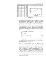
(b) Use the menu command FileJllrint (or the shortcut [Ctrl)+P)
to
bring up the dialog box as shown in Figure
3.1.
In the
Print
what
area, click the
Selection
radio button to specifl that we
wish to print only the selected area.
Figure
3.1
Resistors
1IR
Resistors
1iR
5
02
10
01
15
0066667
25
OM
IRe
0406ti67
Re
2459016
2459016

Re
2 45901
6
Figure
3.2
Printing
a
Worksheet
45
Exercise
3:
Page
Setup
The
Print
Preview
tool
(c) To save both time and paper, and to demonstrate another
feature, we will not click the
OK
button to start the printing
process. Rather, click the
Preview
button. Your screen will
display a picture of how the printed page would look
-
see
Figure 3.2. Note that the gridlines of the worksheet will not be
printed; we can change this later if needed.
Observe what happens when you repeatedly left click within

the Print Preview window: the view is alternately enlarged and
reduced. Use the
Close
button to exit Print Preview.
In this exercise we open the Page Setup dialog box and explore its
many options including: scaling the print job to a specified number
of
pages, setting the margins, requiring that gridlines be printed,
adding headers and footers, the orientation of the paper (portrait or
landscape), etc.
(a)
A
worksheet somewhat larger than the ones we have made
so
far
is
needed to demonstrate one of the features. Go to Sheet6
of CHAP2.XLS where we made the multiplication table. To
extend the table, select
Al:J10
and drag the fill handle down
to row
60.
(b) Use the command FilelPrint Preview or click on the Print
Preview tool. Experiment with the
Next
and
Previous
buttons
in the Print Preview window to see that this worksheet will

print on
two
pages.
(c) Click on the
Setup
button and, if necessary, on the
Page
tab. In
the
Scaring
area, click the
Fit to
radio button and leave the
values in the
two
boxes at
1.
This will cause Excel to shrink
the font size such that your work will fit
on
one page. The
Fit
to
feature does not enlarge, it only shrinks. You can, however,
use the
Adjust to
feature to enlarge the print by a specified
percentage
.
(d) Click on the

Preview
button on the right ofthe dialog box. You
will now find that the worksheet can be printed on one page.
(e) Return to the Page Setup dialog box by clicking on
Setup.
You
will see that Microsoft Excel has adjusted the scaling factor to
85%. To return to the original printed size
(two
pages) you
would need to change this back to
100%.
46
A
Guide to Microsoft Excel
2002
for Scientists and Engineers
Figure
3.3
(f)
Before finishing this exercise you may wish to experiment
with the setting to change the orientation from portrait to
landscape.
Exercise
4:
Changing
(a) With your work showing in Print Preview, experiment with
changing the margins by clicking the ‘Margins’ button. Six
dotted lines appear to show the margin positions. The mouse
pointer shape changes to amagnifying glass until it crosses one

of the margins when it takes on a
9
shape. When
it
has this
shape, hold down the mouse button and drag one of the
margins to a new position.
Margins
(b)
Click again on the ‘Margins’ button to remove the margins
from the view.
Note that there are six margins: left and right, top and bottom,
header and footer. You must be careful not to make the last
two
so
small that the data in the worksheet overlaps the header or footer.
(c) While the method above is useful for a ‘quick-and-dirty’ fix,
it is generally better to set the margins to defined values.
Go
to
the Page Setup dialog box and click the ‘Margins’ tab.
(d) You can set each margin either by typing a new value in the
appropriate box or by clicking the spinners. Set each margin to
one inch (or
2.5
cm) and preview your document.