A Guide to Microsofl Excel 2002 for Scientists and Engineers phần 6 potx
Bạn đang xem bản rút gọn của tài liệu. Xem và tải ngay bản đầy đủ của tài liệu tại đây (856.7 KB, 33 trang )
154
A
Guide to Microsoft Excel
2002
for
Scientists and Engineers
(b) On Sheet4 of CHAP8.XLS enter the text and values
in
A
I
:D3
of Figure
8.15
and the values
in
A4:C7.
In
D4 enter
=RootCount(A4,B4,C4)
and copy it down to row
7.
The values
in column D should agree with those in Figure
8.15.
(c) Constant values may be used as arguments.
To
demonstrate
this, move to an empty cell such as
A10
and enter
=RootCount(l,-5,6).
This should return the value
2.
(d) Move to an empty cell such as
A1
1
and enter
=RootCount(A3,B3,C3).
This will return the error value
#VALUE!.
There are a number of conditions that result
in
this
value. We have passed non-numeric arguments (the cells
A3,
B3, C3 contain text) to a function expecting numeric values.
This error can also be caused by a syntax error
in
the function.
Exercise
7:
The
In
a
looping structure a block of statements is executed repeatedly.
When the repetition is to occur a specified number
of
times, the
FOR
NEXT
structure is used. The syntax for this structure is
FOR
.
N
EXT
Structure
given in Figure
8.16.
Microsoft Excel provides the function FACT to compute
n
factorial. For example, =FACT(4) returns the value of 4!
=
1
x
2
x
3
x
4.
In its absence, we could have coded such a function using
a FOR loop:
Function Fact(n)
Fact
=
1
Forj=l ton
Next
j
End Function.
Fact
=
Fact
*
j
When the loop is first enteredj
is
given a value of
1.
The statement
Fact
=
Fact
*
j
may be confusing at first. Remember that computer
code statements are instructions, not mathematical equations. This
statement may be read as: the new value for
Fact
is its old value
multiplied by
I.
The
Next
statement increments (increases)
j
by
I
and sends the program back to the loop. Another new value of
Fact
is
computed as
Fact
*2.
These steps are repeated until
j
is greater
than the argument
n
at which point the program continues to the
line following the
Next
statement. The reader should see that the
function would be slightly more efficient if the third line read
For
j
=
2
to n.
User-defined Functions
I55
There
is
also
in
VBA
a
FOR
EACH
structure which
is
explored
in
Problem
5
at the end
of
the chapter.
Syntax of FOR .NEXT
For counter
=
first To last
[Step
step]
[statements]
[Exit For]
[statements]
Next [counter]
counter A numeric variable used as a loop counter.
first The initial value of counter.
last The final value of counter.
step The amount by which counter
is
changed each
time through the loop.
statements One or more statements that are executed the
specified number of times.
The step argument can be either positive or negative. If step
is
not specified, it defaults to one.
After each execution of the statements in the loop, step is added
to counter. Then it
is
compared to last. When step
is
positive the
loop continues while counter
<=
end. When step
is
negative
looping continues while counter
>=
end.
The optional Exit For statement, which
is
generally part of an IF
statement, provides an alternate exit from the loop.
Note: If the value of
counter
is altered by a statement anywhere
between the
For
and the
Next
statements, you run the risk of
unpredictable results.
Figure
8.16
For this exercise we will write a function
to
compute the sum of
the squares of the first
n
integers. Our function will find the value
of
12+22+32+
+n20r
Cyk’.
(a) Insert Module5 into the
CHAP8.XLS
project. Code the
function shown in Figure
8.17.
(b) On Sheet5 construct a table similar to that
in
Figure
8.18
to
test your function.
156
A
Guide to Microsoft Excel
2002
for
Scientists
and
Engineers
Exercise
8:
The
DO
.LOOP
Structures
Function SumOfSquares(n)
SumOfSquares
=
0
Forj=lTon
Next
j
SumOfSquares
=
SumOfSquares
+
j
*
2
Figure
8.17
Figure
8.18
The first statement in our function is not really needed because
Visual Basic initializes all numeric variables to zero. However, it
does no harm to perform the initialization explicitly and can make
it easier for another user
to
understand the code.
Whereas the
FOR
.NEXT structure is used for a specific number
of iterations through the loop, the
DO
.LOOP
structures are used
when the number
of
iterations is not initially known
but
depends
on one or more variables whose values are changed
by
the
iterations.
The first syntax
of
the
DO
structure is shown
in
Figure
8.19.
Syntax
1
for
the
DO
statements
Do
{While
I
Until)
condition
[statements]
[Exit
Do]
[statements]
Loop
Figure
8.19
User-dejined Functions
157
From this syntax we see there are
two
variations.
1.
DO
WHILE
condition
LOOP:
Looping continues while the
condition is true. The condition is tested when the first line of
the
DO
statement is executed.
2.
DO
UNTIL
condition
LOOP:
Looping continues until the
condition is true. The condition is tested when the first line
of
the
DO
statement is executed.
Note that the condition is tested at the start of the structure. If the
condition is false, none of the statements
in
the
loop
are executed.
The second syntax tests the condition at the end of the structure
-
Figure
8.20.
Syntax
2
for
the
DO
statements
Do
[statements]
[Exit
Do]
[statements]
Loop
(While
I
Until)
condition
Figure
8.20
This gives rise
to
two
variants:
3.
DO
LOOP
WHILE
condition:
Looping continues while the
condition is true. The condition is tested when the last line of
the
DO
statement (the line beginning with LOOP)
is
executed.
4.
DO
LOOP UNTIL
condition:
Looping continues until the
condition is true. The condition is tested when the last line of
the
DO
statement is executed.
Because the condition is tested at the end of the structure, the
statements within the loop are executed at least once regardless of
the value of the condition at the start of the
DO
structure.
The
two
examples that follow show the difference between Syntax
1
and
2.
With Code
A,
the statements within the
loop
will not be
executed since
t
has a value less than
0.01
when the condition is
tested. With Code
B,
the loop will be entered and the statements
will be executed until
t
<
0.01.
This is true regardless of the value
assigned
to
I
in
the first statement.
158
A
Guide to Microsoft Excel
2002
for
Scientists and Engineers
Code
A
t=O
n=l
sum
=
0
DO
UNTIL
t
<
0.01
t=l/n
sum=sum+l/t
n=n+l
LOOP
Code
B
t=O
n=l
sum
=
0
DO
t=l/n
sum
=
sum
+
1
/t
n=n+l
LOOP UNTIL
t
<
0.01
Typically, the
condition
in
the UNTIL or
WHILE
phrase refers to
one or more variables. The programmer is responsible for ensuring
that the variables eventually have values such that the exit
condition is satisfied. The only exception is when a conditional
EXIT statement is used to terminate the loop.
Consider the code:
t=O
DO
UNTIL
t
>
0.001
statement-I
statement-n
LOOP
Unless there
is
an EXIT
DO
within the loop, at least one
of
the
statements must alter the value off
in
such a way that, after a finite
number
of
iterations,
f
has a value greater than
0.00
1.
If
this is not
the case the loop will execute unendingly.
Ifyou happen to code an infinite
loop
by mistake, your worksheet
will ‘hang
’.
Use
mM
to abort the function.
Have you ever wondered how your calculator, or an application
such as Microsoft Excel, ‘knows’ the value of such quantities as
sin(0.55) or exp(O.456)? The answer
of
course is that they are
calculated from power series. Two examples
of
Maclaurin series
are shown below.
-
(_l)kX*k+’ x3 xs x7
k=O
(2k+1)!
3!
5!
7!
-
Xk
x2
x3
2!
3!
k=o
k!
sin(x)
=
C
-
-
x +
exp(x)
=
C-
=
I
+
x
+
-
+ e.
Of
course, the summations cannot be carried
on
to infinity. The
beauty of these series is that they converge; the terms get
User-defined Functions
159
A
I
B
1
Maclaurin
series
for Exp(x)
2
3x
2
4
MacExpt
7.389056mOI
700
5
Excel
Exp 7.3890560989306500
I
6
Difference\ -4.76063633OE-13
progressively smaller and smaller.
So
we may
use
as many terms
as we need for a specified degree of precision.
In this exercise we will use
a
DO
.LOOP
to code
a
function that
computes exp(x) using the power series shown above. We note
that:
Xk+l
and term,+,
=-
Xk
k!
(k
+
I)!
term,
=-
:.
term,,, =tem,x
-
(3
Thus, we can compute each successive term
From
the one before it.
1 Function MacExp(x)
2 Const Precision
=
0.000000000001
3
MacExp=O
4
Term= 1
5
k=O
6
7
8
k=k+l
9
Do
While Term
>
Precision
MacExp
=
MacExp
+
Term
Term
=
Term
*
x
/
k
10
Loop
11 End Function
Figure
8.21
(a)
On
Module6 enter the code shown
in
Figure
8.2
1
-without the
line numbers, of course. The value in line
2
is
entered as
le-12;
VBA
changes it to the form shown. We have set
Precision
as
a
constant. Walk through the program and follow
it
for
three or four loops to ensure that you follow its workings.
I60
A
Guide
to
Microsoft Excel
2002
for Scientists
and
Engineers
Variables and Data
Types
You can arrange to have
Option
Explicit
automatically added to
every new module. Open
the
-
ToolslOptions dialog
box
in
VBE
and
on
the
Editor tab
place
a
check
mark
beside
Require Variable
Declaration.
(b) Construct a testbed on Sheet6 similar to that shown in Figure
8.22.
Experiment with large and small values in B3. What do
you find? Change the value of
Precision to
1
E-
16 and try large
and small numbers again.
(c) Did you remember to try negative values for
x?
Recall the
advice previously given: thoroughly test every computer
program you write.
So
what happens when
x
is negative? Can
you explain why? The solution is to change line 6 to read:
Do
While abs(Term)
>
Precision. When the argument is negative
the second term is negative and this is smaller than
Precision
so
the loop is terminated after one iteration until we test the
absolute value of
Term.
Unlike most computer languages, all dialects of BASIC allow the
programmer to use variables without first declaring them. While
this feature slightly speeds up the coding process, it has the major
disadvantage that typo errors can go undetected. Suppose a
function uses the variable named
Angle but on one line the
programmer types
Angel. Visual Basic will treat these as
two
different variables and if the error occurs in a long piece of code it
can be difficult to spot. The problem is avoided by the use of the
Option Explicit statement at the start of the module to force explicit
declarations of all variables of every function
in
the module sheet.
With this
in
place, all variables must be declared before being
used. We will use the DIM statement for this purpose.
1 Option Explicit
2 Function MacExp(x)
3 DimTerm, k
4 Const Precision
=
0.000000000001
5
MacExp=O
6
Term=
1
7
k=O
8
9
10 k=k+l
11
13 End Function
Do While Term
>
Precision
MacExp
=
MacExp
+
Term
Term
=
Term
*
x
/
k
12 Loop
Figure
8.23
Figure
8.23
shows the function MacExp from Exercise
8
recoded
to demonstrate this. We do
not
use the function name MacExp, the
User-dejhed
Functions
161
argument
x,
or the constant Precision
in
the dimension (Dim)
statement. The Function statement declares the function name and
arguments, while the Const statement declares its own variable.
Suppose that line
1
1
had been mistyped as term
=
tern
*
x
/
k.
The
cell using this function would show the error value
#NAME?
In
the
module sheet, the word
tern
would be highlighted and the error
message ‘Variable not declared’ would be displayed.
You may wish to consider using this feature in all your functions
or only when the code is long. Remember that after editing a
module, the worksheet must be recalculated by pressing
m.
There is yet another difference from other programming languages.
In
languages such as FORTRAN, C, etc., it is not sufficient merely
to name the variable; the programmer must also state its data type.
In this example we would need to define
k
as an integer variable
and
term
as a floating-point variable. We could do this by coding
line
3 as Dim term
As
Double,
k
As
Integer. When the data type of
variables are not declared Visual Basic uses a special data type
called
variant.
This is acceptable for the simple functions shown
in
these examples but
in
general one should declare data types. It
should be noted that variant data types are memory hogs.
You may wish to use Help to find out more about this topic,
especially the permitted range of values for Integer, Short, Long,
Single and Double.
Exercise
9:
A User-
Function
We may require our user-defined function to return more than one
value or we may wish to pass a range of cell values to a function.
In
this exercise we do both. We will code a function to compute the
real roots of the quadratic equation
ax2
+
bx
+
c
=
0.
defined Array
As
an alternative to the
Option
Base
1
declaration you could use
Dim
Temp(1
to
3).
(a) Insert Module7
in
the CHAP8.XLS project and code the
function shown
in
Figure 8.24.
(b) We will test the function on Sheet7 as shown
in
Figure
8.25.
Only B6:D6 have formulas. Select B6:D6 and type the formula
=Quad(B5,
C5,
D5). This function returns an array,
so
complete the entry with
[Ctrll+[oJ+(EG3].
I62
A
Guide to Microsoft Excel
2002
for Scientists
and
Engineers
A
I
B
I
C
I
D
1 Quadratic Equation Solver
2
-
1
Option Base
1
2
Function Quad(a,
b,
c)
3 Dim Temp(3)
4
d
=
(b
* b)
-
(4
*a c)
5
Select Case d
6
Case
Is
c
0
7
Temp(1)
=
"No
real"
a
Temp(2)
=
"roots"
9 Temp(3)
=
I"'
10 Case
0
11 Temp(1)
=
"One
root"
12
Temp(2)
=
-b
I
(2
*
a)
13 Temp(3)
=
'I"
14 Case Else
15 Temp(1)
=
"Two roots"
16
17
18 End Select
19 Quad=Temp
20 End Function
Temp(2)
=
(-b
+
Sqr(d))
/
(2
*
a)
Temp(3)
=
(-b
-
Sqr(d))
/
(2
*
a)
3
4
5
6
Figure
8.24
ax2
+
bx
+
c
=
0
a b
C
Coeff
1
5
6
Roots
Two roots
-2
-3
(c)
Try
other values for
a,
b
and
c
to test the function. Solve these
equations:
(i)
x2
+
3x
+
3
=
O
(ii)
x2
-
4x
+
4
=
0
(no real roots),
(one real root).
The function contains some new features:
(i)
VBA
does not permit
us
to declare a user-defined function
as an array
so
we use a temporary array to hold the three
values until the end of the function.
(ii)
Note how an array
is
defined in line
3.
This line declares
three variables with the name
temp.
We distinguish one from
the other using an index. Thus we may refer to
temp(Z),
User-deJined Functions
I63
temp(2)
and
temp(3).
In
the absence of the
Option Base
I
statements, these would have been
temp(O), temp(1)
and
temp
(2).
(iii) Values are entered into the elements ofthe array in lines
7
to
17
depending on the value of the discriminant. Some
expressions contain parentheses which are not essential but
aid the reading of the expressions.
(iv)
In
line
19,
the values of the array are passed to the function
to be returned to the worksheet.
The call to the function uses the formula
=Quad(B4, B5, B6). Ifyou
wish to call the function using
=Quad(B4:D4), the function could
be recoded as shown below.
Function Quad(coeff)
Dim Temp(3)
d
=
(coeff(2) 2)
-
(4 * coeff(1)
*
coeff(3))
Select Case d
Case
Is
0
Temp(1)
=
"No
real"
Temp(2)
=
"roots"
Temp(3)
=
""
Temp( 1)
=
"One root"
Temp(2)
=
-coeff(2)
/
(2
*
coeff(1))
Temp(3)
=
""
Temp(
1)
=
"Two roots"
Temp(2)
=
(-coeff(2) + Sqr(d))
/
(2
* coeff(1))
Temp(3)
=
(-coeff(2) - Sqr(d))
/
(2 * coeff(1))
Case
0
Case Else
End Select
Quad
=
Temp
End Function
Exercise
IO:
In
the last part of the previous exercise we saw how to pass a
one-dimensional array to a function. This could be a group of
contiguous cells in a
row
or in a column.
In
this exercise, we pass
Inputting an Array
a two-dimensional array to a function. We pass a block of
12
cells
arranged
in
three rows and four columns to the function which
sums each of the three rows and returns the value of the three
The
FOR
EACHstmcture explored
sums.
in Problem
5
provides another
way
of using ranges as arguments for
a
UDF.
(a)
In
the
VB
Editor, insert Module8 and code the function shown
in Figure
8.26.
164
A
Guide
to
Microsoft Excel
2002
for Scientists and Engineers
1
A
I
B
1
IMaximum
Row
Value
(b)
On Sheet8, enter the values shown
in
Figure
8.27
excluding
D7.
In
D7
enter
=MaxRow(A3:D5).
Check that the function
is
returning the correct value and save the workbook.
C
1
0
1
Option Base
1
2
'Function to return maximum sum
of
three rows
3 Function MaxRow(Data As Object)
4
Dim RowSum(3)
5
Forr=
1
To3
6
Forc=l TO4
7
8
Next
c
9
Nextr
RowSum(r)
=
RowSum(r)
+
Data.Cells(r,
c)
10
MaxRow
=
Application.Max(RowSum)
11
End Function
6
7
Figure
8.26
Largest
row
sum
value
44
91
91
121
81
The code
Data
As
Object
in the argument list
of
the function
references range
A3:D5
in
the worksheet formula.
In
line
4
the
array
RowSum
is created to hold the three values of the
sum
of
each row. The nested FOR loops compute each sum. Note the use
of
Data.Cell(r,c)
to reference the value of each cell
in
the range.
In
line
10,
the worksheet
MAX
function is used to find the largest
value
in
the
RowSum
array.
Exercise
1
I
:
The functions you have written will appear on the Insert Function
dialog box
in
the
User-defined
category but
we
need to make
a
small improvement.
(a) Make
E6
on Sheet
1
the active cell and delete its formula.
Improving Insert
Function
(b)
Click on the Insert Function tool. Select the
User-defined
User-defined Functions
I65
Insert
Function
tool
category and you will see the names
of
all the functions
in
this
workbook. Select the Triarea function. The lower part
of
the
dialog box mistakenly states
Choose the He& button for help
on thisfunction and its arguments.
Click on the
Cancel
button.
(c) Use the command ToolslMacrolMacros
(or
the shortcut
m+m)
to open the Macro dialog box.
In
the
Macro name
box enter the function name
Triarea.
Click on the
Option
button.
In
the
Description
box enter a short description
of
the
functions. Click
OK.
The description is displayed at the
bottom of the Macro dialog box. Close the box using the
@
in
the top right corner.
(d) Use the Insert Function tool to replace the formula
=
Triarea(A6,86, C6)
in
E6.
Note that the Insert Function and the
Function Arguments dialog boxes now display the more useful
information about the function.
Exercise
1
2:
Some
Debugging
Tricks
What do you do when a function returns the wrong value? The first
thing to do is print it out and carefully work through it. The second
thing
is
to find a sympathetic friend, she does not need to be a
programmer, to whom you can explain the function. Many
programmers have found that the act of vocalizing makes you think
more clearly.
You
may find yourself saying to a very puzzled
friend who has said nothing 'Oh! Now
I
see what's wrong. Thanks
for
your help.' When all else fails we need some serious debugging
tools. Very often the problem
is
resolved by examining
intermediate values.
The function
Tritype
which we developed in Exercise
5
requires
that the three sides be sorted in descending order.
If
we make a
mistake
in
the code for that part
of
the algorithm the function will
fail.
In
this exercise we look at
two
methods of checking this part
of
the code.
(a) On Sheet3 enter the value
1
for all three sides
of
the triangle.
(b) Open the
VB
Editor and in the Project Explorer window
double click on Module3 to bring it up
in
the Code window.
(c) Immediately following line
4
(see Figure
8.12)
enter the
statement:
MsgBox
"a
=
"
&
a
&
"
b
=
"
&
b
&
"
c
=
'I
&
c.
This causes the function to display a Message box displaying
the values of the three sides after the sorting has been done.
166
A
Guide to Microsoft Excel
2002
for Scientists and Engineers
The items
in
quotation marks are displayed as text, the values
of the variables
a,
b
and
c
are displayed as numbers. The
ampersands are used to concatenate (join) the textual and
numeric values. Search the term
Msgbox
in
the VBE Help to
learn more about the Message box.
(d) Return
to
Sheet3 and enter the values
4,3
and
5
in
A3, B3 and
C3, respectively. The function
is
recalculated as each value is
entered and each time the function runs it displays the message
box. The third time the box resembles Figure
8.28
and we see
that the three values are indeed sorted correctly.
a=Sb=.lc=3
.
. .
.
,
Figure
8.28
(e)
In
preparation for another debugging method, place a single
quote
in
front of the newly entered code in Module3 to make
it a comment. Replace each value in A3:C3 by
1.
(0
Return to Module3 and edit the new line to read:
If the Immediate window is not visible use the View menu to
bring it up.
Debug.Print
"a
=
"
&
a
&
"
b
=
"
&
b
&
"
c
=
"
&
c
(g) Return to Sheet3 and enter the values
4,3
and
5
in
A3, B3 and
C3, respectively. The function is recalculated as each value is
entered and each time the function runs it prints some output
in
the Immediate window. Open the VBE and the Immediate
window should resemble that in Figure
8.29
and, again, we see
that the three values are indeed sorted correctly.
a=rlb=lc=l
a=4b=3c=l
a=Sb=4c=3
~.
Figure
8.29
User-defined Functions
167
Using Functions
Workbooks
The user-defined functions we have created have been used
in
the
workbook in which they were coded. Every function
in
a workbook
is
available from any sheet
in
it. There are a number of procedures
which permit
us
to use a function from another workbook.
from
Other
1.
The least efficient method
is
to copy and paste the function to
the new workbook.
XLSTART
is a subfolder
of
tht
folder EXCEL in which Excel wa:
installed, generally this will
bt
C:\Program
Files\Microsof
Office\Office
1
O\Excel.
2.
The user-defined functions of an open workbook are available
in other workbooks. Thus if CHAP8.XLS
is
open, then
in
a
second workbook we may code, for example,
=CHAP8,XLS!Quad(.
. .
).
We could either type this formula
or
use the Function Wizard to locate the function in the User-
defined category.
If the workbook containing the modules
is
placed in the
XSTART folder it will automatically open every time
Microsoft Excel
is
started. To make it less obtrusive, use
-
WindowlHide before you save the workbook. When it
is
opened next time it will be invisible. A hidden file can be
made visible again from the Window menu.
<
t
3.
If the functions of workbook CHAP8.XLS are needed
in
only
a few other workbooks the registration method may be more
appropriate. Open workbook CHAP8.XLS and the workbook
.
(let’s call
it
Bookl) in which you wish to use its functions.
In
Project Explorer window of the VB Editor, click on
VBAProject (CHAP8.XLS)
and use ToollVBAProject
Properties to open the
Properties
dialog box. By default, all
You
are not required
to
give the
project the same name as the
workbook,
but
it
is advisable.
projects are named
VBAProject,
but we need a unique name
such as
Chap8.
In the Project Explorer, click on the heading
for the Bookl project and use Toolsl&eference.
In
the resulting
dialog box locate the
CHAP8
project and click the box beside
it. This reference causes CHAP8.XLS to be opened
automatically whenever you open Bookl
.
4.
Finally, we
look
at the steps needed to make an add-in from
CHAP8.XLS once all the functions have been coded and
thoroughly tested.
(i)
In the Project Explorer window, right
click
on
Chap8
(this
assumes you renamed it in Step
3
above) and open the
Properties dialog box. To prevent others from copying
or
modifying your code, enter
a
password on the
Protection
tab.
168
A
Guide to
Microsoft
Excel
2002
for
Scientists and Engineers
(ii)
Return to the Excel window and use FilelPropertjes. On the
Summary,
give the file a descriptive title and add a
documentary remark
in
the
Comment
field.
(iii)
Use FilelSave
As
and
in
the
Type
box select
Microsoft
Excel
Add-in
(it is the last item). The file will be saved with the
extension XLA.
You, and others to whom you give the file, will be able to
use it
in
much the same way as you are using the Analysis
ToolPak add-in.
(iv)
A
number of companies market Microsoft Excel add-ins. For
example, one add-in contains functions for performing mass-
mole chemistry calculations. You may find some shareware
add-ins by searching the World Wide Web.
The procedures above allow you to use worksheet formulas
that refer to functions which are coded
in
another workbook.
Other procedures are needed if you wish to use functions from
another workbook
in
one of your user-defined functions. To
use one of the CHAP8.XLS functions within a function coded
in
Bookl three steps are necessary:
1.
The VPAProject of CHAP8.XLS must be given a unique
name such as
Chap8
-
see
3
above.
2.
With Bookl as the active project
in
the VB Editor, use
-
ToolslReference to reference the Chap8 project.
3.
Within your code, use statements
in
the form
z
=
[Chap8].Macexp,
or
z
=
Macexp.
The first format is
preferred for
two
reasons: it provides better documentation
and it invokes the Auto List Member feature.
Similar procedures allow you to use the functions provided by
the Analysis ToolPak within your own functions.
I.
On the worksheet, use ToolslAdd-ins to load
Analysis
ToolPak
VBA
(note the
VBA
ending).
2.
With Bookl as the active project
in
VBE, reference
atpvbaen
.
3.
Use code
in
the form
z
=
[atpvbaen].Lcm(numbI, numb2).
User-de$ned
Functions
169
2
3
Problems
1
Two
roots
-5
3
1
.*
Write functions with the following properties:
(a) When
A1
contains a temperature value in Fahrenheit,=
Kelvin(A1)
returns the equivalent temperature on the
Kelvin scale. Test the function using
32°F
=
273.15
K
and
(b) When
A2
contains a number n where
n
>>
I,
=Stirling(A2)
returns Stirling’s approximation: In(n!)
=
nln(n)
-
n.
Use
the worksheet
FACT
function to evaluate the accuracy of
Stirling’s approximation.
(c) When
A3
and
B3
contain two integer values
a
and
b,
the
formula
=SumRange(A3,B3)
returns
-459.67”F
=
0
K.
h
En
when
a
I
b
or,
kn
otherwise
n
=u
ii=h
2.*
In
the Quad function of Exercise
6,
line
3
defines a one-
dimensional array
Temp
which
is
passed to the function
Quad
and returned to the worksheet.
In
the worksheet the values are
displayed
in
three cells
in
a vertical arrangement. Thus the
code
Temp(3)
was interpreted as one row and three columns.
We could have made this explicit with
Temp(l,3)
and changed
the references to
Temp(1,l)
=
“No
real”, Temp(l,2)
=
“roots”,
etc.
Use
this information to write
a
modification
of
Quad
(call
it
Quad2)
which could be used as an array formula
in
G2:G4
to give
a
result similar
to
the figure below.
I
I
F
I
G
1
1
lcoeff
I
Roots
1
3.
Write a function to compute the cross-product of
two
vectors.
It should be called using
=CrossProd(VecA,VecB),
where
VecA
and
VecB
are each a vertical range of three cells. This is to be
an array formula returning the three values
in
a vertical range
of three cells. The function header will be
Function
CrossProd(Vect1
As
Object,
Vect2
As Object).
Exercises
9
and
10
will help you get started.
4.
Write a function to use the Newton-Raphson method to find
the real roots
of
a cubic equation, one at a time. The worksheet
should call the function using
=Newton(guess,
a,
b, c, d)
where
I70
A
Guide to Microsoft Excel 2002 for Scientists and Engineers
the arguments are the starting estimate and the coefficients
of
the quadratic equation. The main function should call other
functions to compute
Ax)
and
f’(x).
In
the loop of
Newton,
code an ‘escape hatch’
in
the event thatf’(x) becomes equal to
zero.
5.
In Exercise
7
of Chapter
2
and Exercise
2
of Chapter
5
we
developed a worksheet to find the equivalent resistance of four
resistors
in
parallel. This provides an interesting example to
demonstrate the For Each construct.
Code the following user-defined function and use it
in
a
worksheet similar to that below. The formula
in
E4
is
=Resistor (A3:D3).
This is copied down
two
rows. Note how
the function can handle blank cells. Can
you
modify
it
to also
handle zero values?
Function Resistor(List)
Dim Item
Resistor
=
0
For Each Item In List
If WorksheetFunction.IsNumber(ltem)
Then
End
If
Resistor
=
Resistor
+
1
/
Item
Next Item
Resistor
=
1
/
Resistor
End Function
9
Modelling
I
Concepts
Frequently, physical models are used
in
experiments
to
predict the
behaviour of the real thing. Thus a model aeroplane may be placed
in
a wind tunnel to test the design of a new aircraft.
In
these
experiments, the behaviour of a
system
is being studied. The
system here is the aircraft and the wind that is used to simulate
movement of the aircraft through the atmosphere.
Mathematical models are another way
of
studying the behaviour
of
systems.
You
have often done this yourself. When we use
PV
=
nRTto solve
a
problem, we are assuming that the Ideal Gas Law is
a
good model for the behaviour of
a
gas. However, every model
has its limitations. The ideal gas equation gives poor results at high
pressures and low temperatures; the more complex model of van
der Waals gives a more accurate description under these
conditions. Similarly, Newton’s laws give adequate results unless
the velocities of the objects are moving at speeds approaching the
speed of light; then we need to turn to relativity equations.
In
this chapter we construct and analyse some simple models.
Chapter
10
introduces Solver which may be used for models
requiring optimization.
Exercise
1
:
Model
of
In this exercise we model the behaviour
of
a
bouncing ball. We
begin the design with a description of the system and the objectives
of the model.
a
Bouncing
Ball
Description
A
ball falling from a height, the surface upon which it bounces and
the air through which it moves.
Objective
To generate data showing the maximum height reached by the ball
after
each
bounce.
Now we need to state our assumptions, define the variables of the
problem and state any known relationships between the variables.
As
we do this we may wish to refine the objectives.
I72
A
Guide to Microsoft Excel
2002
for Scientists and Engineers
Assumptions
While we would like the results to be accurate, there
is
a
limit to
the amount of work we are prepared to do for this problem.
So
our
first assumption will be that air resistance may be ignored.
Immediately, we have imposed a limit on the model.
For
a falling
sphere, air resistance
is
negligible when the velocity
is
low. This
means
that our model is ‘good’ only when the initial height is not
large. What other, unstated, assumptions have we made about the
air?
Next we consider the surface. For simplicity, we make this a
smooth, plane surface, perpendicular to the falling ball and rigidly
attached to an object massively larger than the ball.
Now for the interaction of the ball and the surface. Consider a ball
that drops from some height
(h),
hits the surface and bounces back
to a new height
(h’).
In
the idealized case of a perfect elastic
collision
h
=
h‘.
The theory of collisions states that:
Kinetic energy after collision
=
k
x
k%
before collision
(9.1)
where
k
is the coefficient of restitution with
k
=
1
for
a
perfectly
elastic collision and
k<
1
for inelastic collisions. Since the surface
on which the ball falls
is
part of a massive object, we may ignore
any changes in its kinetic energy and from Equation 9.1 derive:
mv2before
kmv2afier
(9.2)
We are interested in the maximum heights reached by the ball after
each bounce. Let
v,,,
refer to the velocity
as
it starts its journey to
reach height
h,
-
the height reached
in
the nth bounce. Then
vbefore
will refer to the velocity of the ball falling from height
h,,
,.
From
the conservation of energy:
mSbefore
=
mgh,_,
and
mv2,fie,
=
mgh,,
We may therefore write Equation 9.2 as:
h,
=
kh,,_,
(9.3)
We now see that our variables are:
h,,
h,,
h,,
and
k
and that
Equation 9.3 relates these variables.
New objective
To generate data showing the maximum height reached by the ball
after each bounce, and to observe how the behaviour changes with
h,
and
k.
The final worksheet will resemble Figure
9.1.
Modelling
I
I73
11
5 11.81
6.55 3.36
1.56
12 6
10.63 5.24
2.35 0.93
25 19 2.70
0.29
0.02
0.00
26
20
2.43
0.23
0.02
0.00
(a) Start
a
new worksheet. Enter the text and values in rows
1
to
4.
The cell C2 holds the value of
h,;
create the name
start
for
this cell.
0.63
0.31
0.00
0.00
(b) Enter the text and values in row
5.
These are the values
of
k
we
are using in the model.
(c) Enter the values
0
to 20
in
column
A.
These number the
bounces.
(d) In
B6
enter the formula
=start
and copy this to
B6:F6.
(e) In
B7
enter the formula
=B$5*B6
and copy this to
B7:F7.
Look
at the formulas in this row. Note how they are in agreement
with Equation
9.3.
(f)
Copy
B7:F7
down to row
26.
(g) We need to test our model.
In
B5
enter the values
0
and
1
.O
successively and note the resulting
h
values. We should get
h,,
=
0
for
n
>
0
when
k
=
0
and
h,,
=
h,
for all
n
when
k
=
1.
Replace the
0.9
value in
B5
after this test.
Figure
9.1
(h)
Make an
XY
chart of the data
in
A5:F26.
(i)
The curves for each kvalue seem to be exponential. To check
this add a trendline to the
k
=
0.9
curve using the options to
display both the equation and the
R2
values on the chart. The
R2
value turns out to be
1
.O
indicating a perfect fit.
I74
A
Guide
to
Microsoft
Excel 2002
for
Scientists and Engineers
(j)
Add trendlines to the other curves with the display equation
option only. The trendlines show the ball obeys the equation:
h,,
=
h,e(cn)
(9-4)
Make a note
of
the
c
value for each
k
value.
If
we examine
Equation
9.3
we see that we could rewrite it as:
h,
=
Ph,
(9.5)
Clearly, the
k
and
c
values
of
Equations
9.4
and
9.5
must be
related.
(k) On a blank part
of
the worksheet, show that the relationship is
c
=
In(k).
Of course, now it
is
obvious: Equation
9.4
could be
written as:
h,,
=
h,
exp(nln(k))
(9.6)
(1)
Save the workbook as
CHAP9.XLS.
In
this model we have observed how the behaviour
of
the system
changes when we vary the value
of
k.
This is called parametric
anaZysis. We could also vary
h,.
There are occasions when we are
unsure
of
the exact value of a variable and make an educated guess
at it. We might then change that parameter
in
small steps and
observe how the behaviour
of
the system changes. This is called
sensitivity analysis.
Exercise
2:
Description
An
ecological niche contains
two
species; one is the prey, the other
the predator.
A
theoretical analysis
of
the problem has yielded
Popu'ation
Mode'
equations for the successive population of the
two
species:
N(t+
I)
=
(
1
.O
-
B(N(t)
-
1
OO))N(t))
-
KN(t)P(t)
P(t>
=
QW)P(t)
where:
N(t)
=
the population
of
prey
in
generation
t
B
=
the net birth-rate factor
K
=
the kill-rate factor
P(t)
=
the population of predators
in
generation
t
Q
=
efficiency
in
use of prey
Objective
To
observe how this model predicts the changing populations and
to
examine the sensitivity
of
the model to the values of the
parameters.
Modelling
I
I75
(a) Open CHAP9.XLS and move to Sheet2. Enter the text and
values shown
in
Figure 9.2. Select the range B6:F7 and use
InsertlNamelCreate to name the cells
in
B7:F7.
Figure
9.2
(b)
We
need some space for
a
graph,
so
move to A37 and enter the
text shown
in
Figure 9.3.
Fill
the range A38:A78 with the
series
I,
2,
,
40.
0.20
-
39
57.50
.~
2t
63.83
I
0.241
Figure
9.3
(c) The formulas
in
B38:C39 are:
B38:
=No
C38:
=Po
C39:
=Q*B38*C38
B39:
=(
1
-
B*(B38
-
100))*838
-
K*B38*C38
(d) Copy B39:C39 down to row 78.
(e)
In
the space below row
8,
create a chart from the data
in
A38:C78 making it 20 rows deep and
8
columns wide. The
chart
in
Figure 9.4 uses
two
y-axes as discussed
in
Exercise
4
of Chapter
6.
The chart shows the classic prey/predator population behaviour:
each species goes to a minimum before rising
to
a
maximum but
the two curves are shifted relative to each other. Note how the
maximum population
of
each species
is
constant.
I76
A
Guide to Microsoft Excel
2002
for
Scientists an& Engineers
Prey and Predator
T
T’O
70
60
%
g50
z40
f
-
$30
0
a
m
0.1
0
:I:::: :::I I::: I::
0.0
10
0
5
10
15
20
25
30
35
Generation
Figure
9.4
(f)
We can now experiment with the parameters. After observing
the effect
of
changing one parameter, re-enter its original value
before changing the next.
(i) Change
N(0)
to
60,
70,
. .
.
(ii) Change
P(0)
to
0.25,0.3,
. . .
(iii) Change
B
to
0.0055, 0.0006,
0.00065,
(iv)
ChangeKto0.25,0.3,0.19,0.18,
Which parameters may be changed slightly while maintaining
a stable state? Can you find one parameter for which a small
change results
in
either a population explosion or an
extinction?
Exercise
3:
Titration
System
Model
A
volume
of
a weak acid (e.g. acetic acid) solution
is
placed
in
a
vessel. Small quantities of a strong base solution (e.g. sodium
hydroxide) are added.
Objective
To
generate the data needed
to
create a chart showing how
the
pH
varies with the volume of base added.
Modelling
I
177
Variables
Ma
the molarity (concentration)
of
the acid solution
Va
the volume
of
acid solution
K,
the dissociation constant
of
the acid
Mb
the molarity (concentration)
of
the base solution
Vb
the volume
of
base solution added
K,
the water constant
1
.O
x
1
0-l4
pH
the pH
of
the solution.
There will
be
several derived variables:
V,
total volume
of
the solution
in
the vessel
Ca
concentration
of
acid remaining after
Vb
ml
of
base solution
has been added
cab
concentration
of
the weak acid's conjugate base
cb
concentration
of
unreacted base after equivalence point.
Relationships
Reaction
of
acid and base
HA
+
NaOH
NaA
+
H,O
Acid dissociation constant
[conc
of
A-]x[conc of H,O+]
[conc
of
remaining
acid HA]
K,
=
Water dissociation constant
K,
=
[conc
of
H,O']
x
[conc
of
OH-
]
Definition
of
pH
pH
=
-log,,[conc
of
H,O']
Assumptions
There are three phases in this system and each has its
own
method
of
calculating the pH:
(i)
The amount
of
base added
is
less than the equivalence point.
If
C,
is
the concentration
of
the remaining acid,
c&
the
concentration
of
A-
(the conjugate base
of
the acid), and
x
the concentration
of
H,O+, then:
HA
+
H,O
+
A
+
H,O'
ca-x
c,,
+x x
I713
A
Guide
to
Microsoft
Excel
2002
for
Scientists and Engineers
Solving the quadratic equation
will
give the concentration of
H,O'
and hence the pH.
(ii)
The equivalence point
when the acid has been exactly
neutralized by the base leaving
a
solution of NaA. If
C,,
is
the concentration
of
A-
and
x
the concentration
of
OH-,
then:
A-
+
H20
+
HA
+
OH-
Ccb
-
x
X
X
Solving the quadratic equation will give the concentration
OH-
from
which
the concentration of
H,O+
and hence the
pH
may be found.
(iii)
Afer
the equivalencepoint
when the
pH
is
dependent only
upon the concentration
of
unreacted base.
If
C, is the
concentration of
OH-
formed from the unreacted base and
x
the concentration
of
H,O+ then
K,=[x][C,]
from which
x
is
readily found.
We will differentiate the three cases with an
IF
function and use
two user-defined functions to solve the quadratic equation
in
the
first two steps. Note that these are required to return only one
value:
(-b+JS)/2a.
(a) Open the
VB
Editor and insert a module on the CHAP9.XLS
project. Code these
two
functions.
Function WeakAcid(CAcid, CConjBase, Acidconstant)
b
=
CConjBase
+
Acidconstant
c
=
-Acidconstant
*
CAcid
WeakAcid
=
(-b
+
Sqr(b
b
-
4
*
c))
/
2
End Function
Function
ConjugateBase(CConjBase,
Acidconstant)
Const
Kw
As
Double
=
0.00000000000001
Baseconstant
=
Kw
/
Acidconstant
b
=
Baseconstant
c
=
-Baseconstant
*
CConjBase
ConjugateBase
=
(-b
+
Sqr(b
*
b
-
4
*
c))
/
2
ConjugateBase
=
Kw
/
ConjugateBase
End
Function