Engineering and Scientific Computations Using MATLAB phần 5 pptx

Chapter
3:
M.4
TUB
and
Problem
Solving
Solution.
The
complex
number
is downloaded
as
81
and
the
plot
is
illustrated in
Figure
3.13.
Chapter
3:
MATLAB
and Problem Solving
82
10
I~
0
I
,

'
,,,,,,
:-~-~~,,''~~
7
6
5
4
1
ipIp-
Lp-L
pp
i
3-
0
500
1000
1500
2000
2500
3000
3500
4000 4500
Figure
3.13.
Nonlinear function: volume versus the external radius
V=JTrl)
0
Example
3.6.6.
Use the

linspace
function and increment method to create a vector
A
with
15
equally spaced
Solution.
Using
linspace,
in the Command Window, we type
values, beginning with
7.0
and
ending with
47.5.
The result is
A=
Columns
1
through 9
7.0000 9.8929 12.7857 15.6786 18.5714 21.4643 24.3571 27.2500 30.1429
Columns
10
through
15
33.0357 35.9286 38.8214 41.7143 44.6071 47.5000
0
Chapter
3:
MATLAB

and
Problem
Solving
83
Example
3.6.7.
Use
linspace
and apply the increment method to create vector
B
with starting (initial) value
of
7
and final (ending) value
of
23
with increment
of
0.16
between values. Display only the 18th value in each
case.
Solution.
Increment method. We enter
Chapter
3:
MATLAB
and
Problem
Solving
84

b. The matrix
E2
is
generated
as
Here, the transpose symbol
'
transforms a horizontal array into
a
vertical one.
Chapter
3:
hrt4T'~
and
Problem Solving
85
Example
3.6.10.
Given matrices A and B
as
A
=
-4
a. A+B
b.
A-B
C.
2*B
d.
A/4

e. A.*B
f.
B.*A
g. A*B
h.
B*A
k.
A."2
1.
A"2
m. A."B
n.
A./B
using pencil and paper. Verify the results using
MATLAB.
Solution.
First,
we download matrices A and B
as
,
calculate
the
following:
-5
31
Chapter
3:
MATLAB
and Problem
Solving

86
Chapter
3:
MATLAB
and Problem
Solving
87
Chapter
3:
MATLAB
and Problem
Solving
88
Chapter
3:
MATLAB
and
Problem
Solving
89
Chapter
3:
MATLAB
and Problem
Solving
90
Example
3.6.13.
Write an m-file which will generate a table of conversions from inches to centimeters using the
conversion factor

1
inch
=
2.54
em. Prompt the user to enter the starting number of inches. Increment the inch
value by
3
on each line. Display a total of
10
lines. Include a title and column heading in the table.
Solution.
The m-file should be written. Fiurthermore, to execute an m-file,
MATLAB
must be able to find it.
This means that a directory in
MATLAB'S
path must be found. The current working directory is always on
the path.
To
display or change the path, we use the
path
function.
To
display or change the working
directory, the user must use
cd.
As
usual,
help
will provide more information.

To solve the problem, the following m-file
is
written. Comments are identified by the
%
symbol.
Chapter
3:
MATLAB
and Problem Solving
91
Example
3.6.14.
Write an m-file that will calculate the area of circles
(A
=
x?)
with radii ranging from
3
to
8
meters
at an increment between values entered by the user in the Command Window. Generate the results in a table
using
disp
and
fprintf,
with radii in the first column and areas in the second column. When
fprintf
is used, print the radii with
two

digits after the decimal point and the areas with four digits after the decimal
point.
Solution.
To
solve the problem, the
MATLAB
script is developed and listed below.
Chapter
3:
MATLAE
and
Problem
Solving
92
Example
3.6.15.
Write an m-file which allows the user to enter (download) the temperatures in degrees Fahrenheit
and return the temperature in degrees Kelvin. Use the formulas
C"
=
5(F"- 32)/9
and K
=
C"
+
273.15.
The
output should include both the Fahrenheit and Kelvin temperatures. Make three variations of the output
as:
a.

b.
C.
Output temperatures
as
decimals with
5
digits following the decimal point,
Output temperatures in exponential format with
7
significant digits,
Output temperatures with
4
significant digits.
Solution
The following
MATLAB
script allows us to solve the problem:
Chapter
3:
MATLAB
and
Problem
Solving
The results displayed in the Command Window are documented below:
the height
of
Y=
3
J
Enter the three

radii
in meters:
2
31
R=
93
t=
20
2.8794 20.8627 57.6956
The three
volumes
are
found to
be
2.8794,20.8627, and 57.6956.
Chapter
3:
MTLAB
and Problem Solving
94
Example
3.6.18.
cone with those dimensions.
Write a
MATLAB
script which accepts the
radius
and
height
as

inputs
and
returns the volume
of
the
Solution.
The script
(ch3618
.m)
is
given below.
Chapter
3:
MATLAB
and Problem
Solving
95
Example
3.6.20.
Write the
MATLAB
file to solve linear algebraic equations. Develop
an
m-file in order to solve the
following sets of linear algebraic equations:
a.
6~- 3y
+
42= 41
12~

+
5y
-
72
=
-
26
-
5x
+
2y
+
6z= 14
b.
12x-5y=
11
-
3x +4y
+
7z=
-
3
2.5%
+
5x3
+
XI
-
2x2=,4
6x+2y+3z=22

25x2
-
6.2~~
+
18%
+
1
Oxl
=
2.9
C.
28%
+
25x1
-
30x2
-
15x3
=
-
5.2
-3.2~1+ 12~,-8~q=-4.
Solution.
The following m-file
is
written:
Thus,
the solutions of the algebraic equations are found.
Chapter
3:

MATLAB
and
Problem
Solving
96
Example
3.6.21.
Electric circuits are described (modeled) using Kirchhoffs voltage and current laws. The electric
Rlil
+
R2i2- v,
=
0
-
R2i2
+
R3i3
+
R5i5
=
0
v2
+
R&-
R3i3=
0
-
i,
+
i2+ i3+

i4=
0
-
i4-
i3
+
i5
=
0
Calculate the five unknown currents
(il,
i2,
i3,
i4,
and
is)
using the following resistances and voltages
as:
Rl
=
470
ohm,
R2
=
300
ohm,
R3
=
560
ohm,

R4
=
100
ohm,
R5
=
1000
ohm,
v1
=
5V,
and
v2
=
I
OV.
Label the answers with current number and units.
.
Using the resistances given above and
vI
=
5V,
find the range of positive voltages
v2
for which none
of
the currents exceeds
50
mA.
The currents may be positive or negative. None of the currents may

be less than
-
50
mA or greater than
50
mA.
Solution.
The
MATLAB
script is documented below.
circuit under consideration is described by the following set of five algebraic equations:
a.
b.
Chapter
3:
MTLAB
and
Problem
Solving
The results are
97
Example
3.6.22.
The height, horizontal distance, and speed
of
a projectile launched with a speed
v
at an angle
A
to the

h(t)=vtsinA-igt2, x(t)=vtcosA
and
v(t)=,/v2 -2vgtsinA+g2t2
.
The projectile will strike the ground when
h(t)
=
0,
and the time
of
the hit
is
t,,,,
=
2-sin
A
.
horizontal line are given by the following formulas:
V
g
Suppose that
A
=
30°,
v
=
40
m/s,
and
g

=
9.81
m/s2. Use logical operators to find the times (with
The height is no less than
15
meters,
The height is no less than
15
meters and the speed
is
no greater than
36
m/sec.
Solution.
The following
MATLAB
script is developed to solve the problem.
the accuracy to the nearest hundredth of a second) when
a.
b.
Chapter
3:
MATLAB
and
Problem
Solving 98
REFERENCES
1.
2.
3.

4.
5.
MTUB
6.5
Release
13,
CD-ROM, Mathworks, Inc.,
2002.
Hanselman,
D.
and Littlefield,
B.,
Mastering
MATLAB
5,
Prentice Hall, Upper Saddle River,
NJ,
1998.
Palm, W.
J.,
Introduction to hi4TLABfor Engineers,
McGraw-Hill,
Boston,
MA,
2001.
Recktenwald G.,
Numerical Methods with MATLAB: Implementations and Applications.
Prentice Hall,
Upper Saddle River,
NJ,

2000.
User’s Guide. The Student Edition
of
MATLAB:
The Ultimate Computing Environment for Technical
Education,
Mathworks, Inc., Prentice Hall, Upper Saddle River, NJ, 1995.
Chapter
4:
MATLAB
Graphics
12
10-
8-
6-
Chapter
4
/",
-
'
MATLAB
GRAPHICS
99
MATLAB
has outstanding graphical, visualization and illustrative capabilities
[
1
-
41.
A

graph is a collection
of
points,
in
two,
three, or more dimensions, that may or may not be
connected by lines or polygons. It was emphasized that
MATLAB
is designed to work with vectors
and matrices rather than functions. Matrices are a convenient way
to
store numerical numbers.
4.1.
Plotting
In
MATLAB,
the user can plot numerical data stored as vectors and matrices. This data can
be obtained performing numerical calculations, evaluating functions, or reading the stored data
fi-om files. Single and multiple curves can be created.
The dependent variable can be easily evaluated as a function
of
the independent variable.
For example, consider
y(x)
=AX),
e.g., y(x)
=
x"~,
y(x)
=

x2, y(x)
=
e-x,
y(x)
=
sin(x), etc.
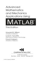
To create a line plot ofy versus x, the
MATLAB
statement is
we obtain the plot as documented in Figure
4.1
.b.
141
'\
,/

'-
\I
1
i
a
Figure
4.1.
Data plots
b
0
By default, the
plot
function connects the data with
a

solid line. Using
plot
(x,
y,
'
or
)
,
the data is connected by symbol
0.
Chapter
4:
MATLAB
Graphics
100
As
has been shown,
plot
is the simplest way
of
graphing and visualizing the data.
If
x
is
a
vector,
plot
(x)
will plot the elements
ofx

against their indices. For example, let
us
plot the
vector. We type
The resulting graph is displayed in Figure
4.4.
Chapter
4:
MATLAB
Graphics
101
Figure
4.4.
Plot of two vectors
x
and
y
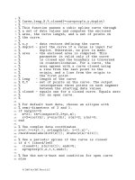
Let us illustrate how to calculate the function
x(t)
=
L'sin(2t) if
t
varies from
0
to
8
sec,
and then plot the resulting function. We will use the colon notation
(:
is the special character) to

create the time array. For example, typing
t=O
:
1
:
8,
we have
The
resulting
plot
is
illustrated in the Figure
4.5.
Chapter
4:
MATLAB
Graphics
102
05-
',
04-
03-
02-
01-
l
0
1
2
3
4

5
6
7
a
-0.2-
'
Figure
4.5.
Plot of the function
x(t)
=
e-'sin(2t)
The function
plot (t,
x)
uses the built-in
plot
function and gives a very basic plot.
The first variable is on the horizontal axis and the second variable is on the vertical axis. There
are many ways to use
plot.
For example, you can change the style and color
of
the line. Using
plot
(t
,
y,
:
I

)
gives the dotted line. To have the green dashdot line, type
plot (t,
x,
g-
.
I).
The following options are available:
solid
-
red r
dashed

green
9
dotted
:
blue
b
dashdot

white
W
We can use the
help
plot
for detail information. That is, using
Chapter
4:
MATLAB

Graphics
Line
-
solid
103
Color
Symbol
y yellow
.
point
The results are integrated in Table
4.1.
I
:
dotted
I
m
magenta
I
o
circle