Engineering and Scientific Computations Using MATLAB phần 6 ppt

Chapter
4:
MATLAB
Graphics
104
To
illustrate the
plot
function and options we have, using the
MATLAB
statements
L'':
17
08-
06
04
02
Or
I
-021
-0
4
-0
61
I
-0
8
b
-11
-LA
L-i-

-I-&
12
3
4
5 6
7
8 9
10
L'':
17
08-
06
04
02
Or
I
-021
-0
4
-0
61
I
-0
8
b
-11
-LA
L-i-
-I-&
12

3
4
5 6
7
8 9
10
Figure 4.7.
Plot
of
sin(n)
Thus,
two-
and three-dimensional (as will be illustrated latter) plots and coordinate
transformations are supported
by
MATLAB.
The basic commands and fbnctions are reported in
Tables
4.2
to
4.5.
Chapter
4:
MATLAB
Graphics
Table
4.2.
Basic Plots and Graphs Functions and Commands
105
Horizontal bar chart

Table
4.3.
Three-Dimensional Plotting
Table
4.4.
Plot
Annotation and Grids
Chapter
4:
MATLAB
Graphics
106
contour
contourc
contourf
hidden
Table
4.5.
Surface, Mesh, and Contour Plots
Contour (level curves) plot
Contour computation
Filled contour plot
Mesh hidden line removal mode
mesh
peaks
surf
surface
surfc
surf1
trime sh

I
meshc
1
Combination mesh/contoumlot
I
3D
mesh with reference plane
A sample function of two variables
3D
shaded surface graph
Create surface low-level objects
Combination surf/contourplot
3D
shaded surface with lighting
Trianeular mesh dot
05-
O!
I
trisurf
I
Triangular surface plot
'
Let
us
illustrate the
MATLAB
application within an example.
Illustrative Example
4.
I.

3.
Calculate and plot the function
f(t)
=
sin(1 OOt)e-*'
+
sin(100t)cos(100t
+
I)e-",
0
I
t
I
0.1
sec.
Solution.
To calculate and plot the fimction
f(t)
=
sin(1 OOt)e-2'
+
sin(lOOt)cos(l
OOt
+
l)e-5' for
0
I
t
I
0.1

sec, we assign the time interval of interest
(0
I
t
I
0.1
sec), calculateJ(t) with the desired
smoothness assigning increment (for example,
101
values), and plot this fbnction. We have the
following statement:
The resulting plot forfit) is given in Figure 4.8.
1,
I
-0.5
1
'%,
.
I
-2
~
I
0
0.02
0.04
0.06
0.08
0.1
Figure 4.8. Plot of the hnction
f(t)

=
sin(100t)e-2'
+
sin(lOOt)cos(lOOt
+
l)e-5'
0
One can change the type of line used to connect the points by including a third argument
-'
solid
dotted line, and
-
.
'
dashdot line. The default line type
specifying line type. The syntax
is
plot
(x,
yf
'
-
'
)
.
The line types available are:
line (default),
I I
dashed line,
I

:
Chapter
4:
hit4
TLAB
Graphics
107
is solid. However, a graph
is
a discrete-time array. One can use a mark to indicate each discrete
value. This can be done by using a different set
of
characters to specify the line-type argument. If
we use a
'
.
'
,
each sample
is
marked by a point. Using a
+
marks each sample with a
+
sign,
*
uses stars,
o
uses circles, and
x

uses x's. For example, assigning the time interval
t=O
:
1
:
12,
let
us calculate x
=
sint, and plot the function. We have
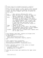
The resulting plot
is
illustrated in the Figure 4.9.
-021
-0.4
1
i
I
I
-061
4
-0
8
-1
/I
I
-
ti
-
I

L-S-J
2
4
6
a
10
12
0
Figure 4.9. The plot of x
=
sint
We can also plot several graphs on the same axis. For example, let us calculate and plot
two
functions x
=
sint and
x
=
sin(0.5t). We type
>>
t=0:.25:12; xl=sin(t); x2=sin(0.5*t); plot(t,xl,t,xl, '+',tlx2,t,x2,
'0')
and the resulting plots are illustrated in Figure 4.10.
Figure 4.10. Plots of x
=
sint and x
=
sin(0.5t)
The user can change the axes scale, and the logarithmic scale functions are the following:
0

loglog
(logarithmic
x-
and y-axis scale),
0
semi
1
ogy
(linear x-axis and logarithmic y-axis scale),
0
semilogx
(linear y-axis and logarithmic x-axis scale).
Chapter
4:
MATLAB
Graphics
108
We can have the text labels on the graphs and axes. The following labeling statements are
used for title,
x-
and y-axis:
The plot is illustrated in Figure
4.1
1.
Function
x(t)
T
-
I
,

I-
3
~~~~
r
"Li
I
"0
5
10
15
20
25
30
t
(time)
2
+
sin
t
4.05,
Figure
4.1
1.
Plot
of
the function
x(t)
=
e
,OItI30

2-costt
The
commonly used annotation hnctions are listed in Table
4.6.
Chapter
4:
MATLAB
Graphics
109
Table
4.6.
MATLAB
Annotation Functions
The
plot
function allows us to generate multiple curves on the same figure using the
plot(xl,yl,sl,x2,y2,
I
following syntax
where the first data set represented by the vector pair
(XI, yl
)
is plotted with the symbol
definition
sl,
the second data set
(x2, y2
)
is
plotted with symbol definition

s2,
etc. It should
be emphasized that the vectors must have the same length (size). Thus, the length of
xl
and
yl
must be the same. The length (size) of
x2
and
y2
must be the same, but in general, can be
different from the length of
xl
and
yl.
The separate curves can be labeled using
legend.
Illustrative
Example
4.1.5.
Calculate and plot
two
functions
x,
(0
=
Solution.
The following
MATLAB
script is developed:

2
+
sin
t
-0
05,
2+sint
-02,
e
,O<t<30 and
x2(t)=
e
,O<t130.
2
-
cosit
2
-
cosit
The resulting plots are shown in Figure
4.12.
Functions
xl(t)
and
x2(t)
3
I
,
‘I
0

I
-A-
L.
A
I/
0
5
10
15
20
25
30
1
(time)
Figure 4.12. Plots of functions
Chapter
4:
MATLAB
Graphics
1
10
The
axis
command
is
used to control the limits and scaling of the current graph. Typing
axis
(
[min, maxx min, max,]
we assign a four-element vector to set the minimum and maximum ranges for the axes. The first

element
is
the minimum x-value, while the second
is
the maximum x-value. The third and fourth
elements are the minimum and maximum y-values, respectively.
Let us calculate
(for
OSt
530
sec) and plot (in O<t
520
sec) functions
2
+sint
e
.
The plots should be plotted using the x-axis
2
+
sin
t
-0.051
e and x2(t)
=
XlW
=
2
-
cosa

t
2
-
cosa
t
from
-1
to
3.
The following
MATLAB
script is used:
The plots are documented
in
Figure
4.13.
3
2
-

v
N
u
m
XI
TO
p
-1
X
0

m
._
2
u-
-1
-1
._
I
\
Functions
xl(t)
and
@(t)
0
5
10
t
(time)
15
20
2
+
sin
t
-0,05r
2
+
sin
t
Figure

4.13.
Plots of
xl (t)
=
e
and
x2(t)=
e
2
-
cosat
2
-
cosat
It was illustrated that
MATLAB
provides the vectorized arithmetic capabilities.
Illustrative Example
4.
I.
6.
X
X
Calculate functions
f,
(x)
=
-
and f,(x)
=

if-55x55.
1
fX4
1
+sin x
+
x
Solution.
We have the folowing statement:
>>
x 5:0.25:5;
fl-x.
=x,
/
(l+sin
(x)
+x.
^4)
;plot
(x,
fl,
'
+
I,
x,
f2,
'0'
)
The graphs
of

these two functions are illustrated in Figure
4.14.
Chapter
4:
MTLAB
Graphics
111
X X
Figure
4.14.
Plots of the functions
A(X)
=-
and
f2(x)=
,-51x15
0
1+x4
l+sinx+x4
The
hold
command will keep the current plot and axes even if
you
plot another graph.
Let
us
calculate the nonlinear functions x(t)
=
-
cos(t

+
z)
,
y(t)
=
1
I
sin(t
+
x)
and plot them if
-
1On
I
t
I1
On
.
Then, holding the plot, calculate the function
lOe",
for
z
=
-
0.01
+
0.5i
to
z
=

-
1
+
50i
(z
is
the complex variable, and let the size of the
z
array be
991).
Plot
the function
1
Oe".
The
MATLAB
script is given below, and the resulting plots are given in Figure
4.15.
The new graph will just be put on the current axes.
sin
50t
I
sint50t
I
-8,
-20 -10
0
10
-30
i

-10
-40
-50
Figure
4.1
5.
Functions plots
Chapter
4:
MA
TUB
Graphics
1
12
Plotting
Multiple Graphs.
The subplot command allows the user to display multiple
plots in the same window and print them together. In particular, subplot
(m,
n,
p)
partitions
the figure window into an m-by-n matrix of subplots and selects the pth subplot for the current
plot. The plots are numbered along first the top row of the figure window, then the second row,
and
so
on. The order for
p
is
as follows:

121.
Thus, subplot partitions the window into
LIJ
multiple windows, and one or many of the subwindows can be selected for the specified graphs.
In general, subplot divides the graphics window into the specified number of quadrants.
As
mentioned, m.is the number of vertical divisions, n
is
the number of horizontal divisions, and
p
is
the selected window for the current plot (p must be less than or equal to
m
times n). For
example, subplot
(
1,
2,
1
)
will create two full-height, half-width windows for graphs, and
select the first (left window) as active for the first graph.
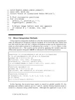
To plot the data, the basic steps must be followed. To illustrate the
MATLAB
capabilities,
we study the modified previous example with the sequential steps as documented in Table
4.7.
Chapter
4:
MATLAB

Graphics
113
To
plot the functions, the
ezplot
plotter
is
also
frequently used. Let
us
plot the function
y
=
sin4 xcosx+e-l”I c0s4
x
using
ezplot.
To
plot this function, we type
Chapter
4:
MATLAB
Graphics
1
14
As
given in the
MATLAB
help, to create a helix, we type in the Command Window
Chapter

4:
MATLAB
Graphics
115
The three-dimensional plot
is
documented in Figure
4.1
8.
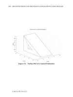
Figure 4.18. Three-dimensional plot,
i(x,
y)
=
x2ye-xz-y2
if
-41x14 and
-41~14.
Illustrative Example
4.2.1.
Calculate and plot the sinc-like function
z(x,
y)
=
sin
x
+y
+E
7,
&=lxlO-'O
if

4-
-1O<x<lO and
-1O<y110.
Solution.
We apply
meshgrid,
plot3
and
mesh.
In particular, making use
of
>>
[x,y]=meshgrid(
[-10:0.2:10])
;xy=~qrt(x.~2+y.~2)+le-10;z=sin(xy)
./xy;plot3(x,y,z)
>>
[x,
y] =meshgrid(
[-1O:O.
2:
101
)
;xy=sqrt (x.
"2+y.
"2)
+le-10; z=sin
(xy)
.
/xy;mesh

(z)
and
the three-dimensional plots are illustrated in Figure
4.19.
Chapter
4:
MATLAB
Graphics
1
16
sin
Jx'
+
y2
+
E
Figure
4.1
9.
Three-dimensional plots of
z(x,
y)
=
0
JXjG
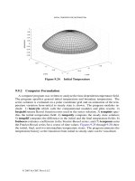
Using the subplot commands, let
us
plot four mesh-plots. We have the following
MATLAB
statements

and the corresponding three-dimensional plots are documented in Figure
4.21.
Chapter
4:
MATLAB
Graphics
117
mesh
plot
surfc
plot
surf
plot
-10
-10
-10-
-10
-
Figure4.21. Plotof z(x,y)=l-+x2-+y2 if -101x110 and -1OIyIlO
MATLAB
creates a surface by calculating the z-points (data) above a rectangular grid in
the
xy
plane. Plots are formed by joining adjacent points with straight lines.
MATLAB
generates
different forms of surface plots. In particular, mesh-plots are wire-frame surfaces that color only
the lines connecting the defining points, while surface plots display both the connecting lines and
the faces of the surface in color. Functions
mesh

and
surf
create surface plots,
meshc
and
surf
c
generate surface plots with contour under-plot,
mesh
z
creates surface plots with curtain
plot (as the reference plane),
pcolor
makes flat surface plots (value
is
proportional only to
color),
surf
1
creates surface plots illuminated from a specified direction, and
surface
generates low-level hnctions (on which high-level functions are based) for creating surface
graphics objects.
The
mesh
and
surf
functions create three-dimensional surface plots of matrix data.
Specifically, if
2

is a matrix for which the elements
Z(ij)
define the height of a surface over an
underlying
(ij)
grid, then
mesh
(
Z
)
generates and displaces a colored, wire-frame three-
dimensional view of the surface. Similarly,
surf
(Z)
generates and displaces a colored,
faceted three-dimensional view of the surface.
The functions that generate surfaces can use two additional vector or matrix arguments to
describe surfaces. Let
2
be an rn-by-n matrix,
x
be an n-vector, and
y
be an m-vector. Then,
mesh
(x,
y,
Z,
C)
gives a mesh surface with vertices having color

C(ij)
and located at the
points (xv),
y(i),
Z(ij)),
where
x
and
y
are the columns rows of
2.
If
X,
K
2,
and
C
are matrices of the same dimensions, then
mesh
(X
,
Y,
Z
,
C
)
is a mesh
surface with vertices having color
C(ij)
located at the points

(X(ij),
Y(ij),
Z(ij)).
Using the spherical coordinates,
a
sphere can be generated and plotted applying the
Hadamard matrix (orthogonal matrix commonly used in signal processing coding theory). We
have the
MATLAB
statement as given below,
and Figure 4.22 illustrates the resulting sphere.
Chapter
4:
MATLAB
Graphics
1
18
-1
-1
Figure 4.22. Three-dimensional sphere
Finally we illustrate two- and three-dimensional graphics through examples as given in
Table 4.8.
Table 4.8.
MATLAB
Two- and Three-Dimensional Graphics
Problems
with
MATLAB
Syntax
>>

x=-10:0.1:10; y=x.^3; plot(x,y)
>>
t=-10:0.1:10;
>>
x=t
.^2;y=t .^3;z=t
4;
plot3
(x,
y, z)
;
Plot
loow
1
aooo
4000
I
,
-500
-1000
0
Chapter
4:
MATLAB
Graphics
119
>>
t=-Z*pi:O.l:2*pi;
,>
x=sin(t); y=cos(t); plot(x,y)

>>
t=-Z*pi:O.l:Z*pi;
>>
x=sin(t) .*cos(t); y=cos(t);
’>
plot(x,y)
>>
t=-lO*pi:O.l:lO*pi;
>>
x=sin(t)
;
y=cos (t)
;
z=t;
>>
plot3 (x,
y,
z)
>>
t=-5*pi:O.l:5*pi;
>>
x=sin(t) .*cos(t);
>>
y=cos (t)
;
z=t;
>>
plot3 (x, y,
2)
,

,’
-04‘
/”
-0
6
.40<
0.5
-1
-1
-
-1
-05
Chapter
4:
MA
TLAB
Graphics
120
>>
t=-lO*pi:O.l:lO*pi;
>>
x=sin(t)
;
y=cos (t) .*cos (t)
;
>>
z=sin
(t)
. *cos (t)
;

>>
plot3
(x,
y,
z)
>>
t=-lO*pi:O.l:lO*pi;
>>
x=sin
(t)
.*sin
(t)
;
>>
z=sin
(t)
.
*cos
(t)
;
>>
y=cos (t)
.*cos
(t)
;
>>
*plot3 (x, y,
z)
>>
y=cos

(t)
.*cos
(t)
;
>>
z=exp(-t) .*sin(t) .*cos(t);
>>
plot3
(x,
y,
z)
>>
t=linspace (-2,3,50)
;
>>
[x,yl=meshgrid(t,t);
>>
z=-l./(l+x.^4+~.~4) ;contour3(z);
05
0
-0
5
1
,
03i
\
\
00
Chapter
4:

MATLAB
Graphics
121
1
-r-j
aak
a4
/
\-
04-
Q6-
'\
a6
\~
a2
i-
02,
Or
0
r-
MATLAB
has animation capabilities. Advanced animation functions, commands and examples are
As illustrated in Table
4.8,
the circle was calculated and plotted using the
MATLAB
statement
reported
in
the specialized books and user manuals. Let us illustrate the simple examples.

1
_
,
,
,
\
'\!
-\
,
I
I
Figure 4.23. Bead location and circular path
Using
movie, moviein,
and
getframe,
the movies can be made.
In
particular, the
animated sequence of plots are used to create movies. Each figure
is
stored as the movie frame,
and frames (stored
as
column vectors using
getframe)
can be played on the screen. The
generalized and specific
MATLAB
scripts are given below

Nframes=3;
%
assign the number of frames
Mframe=moviein(Nframes);
%
frame matrix
for i=l:Nframes
x=[
I;
y=[
1;
z=[
1;
%
create the data
plot3 (x,y,
z)
or plot
(x,y)
;
%
other 3D and 2D plotting can be used
Mframes
(:,
i)=getframe;
end
N=2
;
movie (Mframe, N)
%

play the movie frames N times
and
t=-2*pi:O.l:2*pi;
Nframes=3;
%
number
of
frames
Mframe=moviein(Nframes);
%
frame matrix
for i=l:Nframes
x=sin (t)
;
y=cos (t)
;
%
data
Mframes
(
:,
i) =getframe;
end
for
j=1
:Nframes
x=sin(t); y=sin(t) .*cos(t);
%
data
Mframes(:,j)=getframe;

end
N=2
;
movie (Mframe,N)
%
play the movie frames N times
plot
(x,
Y)
;
plot
(x,
Y)
;
The resulting frames are documented in Figure 4.24.
Chapter
4:
MATLAB
Graphics
122
Figure 4.24. Movie frames
It is obvious that
for
loops
can be used.
A
simple example is given below to clculate the
quadratic function
x2
in the region from

-
8
to
8
and increment 2. We have the following
MATLAB
statement,
for
i=-8:2:8
end
and the numerical values are given below:
i=
x=iA2; i, x
-8
64
x=
i=
-6
36
-4
16
x=
i=
x=
Chapter
4:
MATLAB
Graphics
123
16

%
data
As
an illustrative example, the reader
is
advised to use the following
MATLAB
script to
create a “movie”.
t=-2*pi:O.l:2*pi;
Nframes=50;
%
number of frames
Mframe=moviein(Nframes);
%
matrix frame
for i=l:Nframes
x=sin(lO*i*t)
;
y=cos (10*i*t);
Mframes
(:,
i)=getframe;
end
for j=l:Nframes
x=sin (2* j*t)
;
y=sin (4* j*t)
.
*cos (6* j*t)

;
%
data
Mframes
(:,
])=getframe;
end
N=2
;
movie (Mframe,N)
%
play the movie frames
N
times
Four of the resulting frames are given in Figure
4.25.
i=O; j=O;
i=i+l;
plot (x, Y)
;
j=j+l;
plot (x, Y)
;
0
0
0
a
n
Q
n

n
I
05
o
05
1
1n50051
Figure
4.25.
Four movie frames
Another example which can be used
is
based
on
the
MATLAB
script given below
t=-2*pi:O.l:2*pi;
Nframes=5;
%
number
of
frames
Mframe=moviein(Nframes);
%
matrix frame
for i=l:Nframes
i=i+l
;
i=O;

j=O;
for j=l:Nframes
j=j+l;
x=sin(i*j*t); y=cos(i*j*t);
%
data
Chapter
4:
MATLAB
Graphics
124
plot (x, y)
;
Mframes(:,i)=getframe;
end
N=2
;
movie (Mframe,N)
%
play the movie frames
N
times
end
The
MATLAB
script which makes the three-dimensional "movie" is documented below:
t=-3:0.05:3;
Nframes=6;
%
number of frames

Mframe=moviein(Nframes);
%
matrix frame
for i=0:2:Nframes
[x,y]=meshgrid( [t]
)
;
xy=sqrt(x.^(iA2)+y.^ (i^2) )+le-5; z=sin(xy) ./xy;
plot3(x,y,z);
Mframes
(
:,
i) =getframe;
end
for
j
=O
:
2
:
Nf rame
s
j=j+2;
[x,
y]
=meshgrid
(
[
t
]

)
;
xy=sqrt(x."(2*j)+y."(4*j))+le-5;
z=cos(xy).*sin(xy)./xy;
plot3 (x, y,
z)
;
Mframes(:,j)=getframe;
end
N=2
;
movie (Mframe,N)
%
play the movie frames N times
i=O;
j=O;
i=i+2;
To create a graph of a surface in three-dimensional space (or a contour plot of a surface),
it was shown that
MATLAB
evaluates the function on a regular rectangular grid. This was done by
using
meshgrid.
For example, one creates one-dimensional vectors describing the grids in the
x-
and y-directions. Then, these grids are spead into
two
dimensions using
meshgrid.
In

parti cu
1
ar,
Using the
meshgrid
comand, we created a vector
X
with the x-grid along each row, and
a vector
Y
with the y-grid along each column. Then, using vectorized functions and/or operators,
it is easy to evaluate a function
z
=Ax,y)
of two variables (x and
y)
on the rectangular grid.
As
an
example,
i>
z=sin(X)
.*cos(Y) .*exp(-O.O01*X."2);
Having
created the matrix containing the samples
of
the function, the surface can be graphed
using either
mesh
or the

surf,
>>
mesh
(x,
y,
z)
>>
surf
(x, y,
z)
and the resulting plots are given in Figures 4.26.a and b, respectively. The difference
is
that
surf
shades the surface, while
mesh
does not.
Chapter
4:
WTLAB
Graphics
125
_.
__
I ,
-
_
I
-_
_

I
40
40
00
00
a
Figures 4.26. Three-dimensional plots
b
In addition, a contour plot can be created using the
contour
function, as in Figure
4.27.
Chapter
4:
MA
TLAB
Graphics
126
The resulting plot
is
shown in Figure
4.28.
Sinusoidal function
T-
-7-
7
T
-
-I
I

I
I
I
I
I
,
I
1
time,
t
[second]
Figure
4.28.
Plots
of
functions
x(t)
=
2
+
3
sin(nt
+
10)e-0.35'
Example
4.3.2.
Calculate and plot the discrete function
x(n)
=
25

cos(m
+
5)e4.1fl
if
0
5
n
I
40.
Solution.
The
following
MATLAB
script
is
developed using the
stem
function:
The
resulting plot is documented in Figure
4.29.
0
5
10
15 20 25
30
35
40
Figure
4.29.

Plots
of
functions
x(n)
=
25cos(m
f5)e-O."