Statistical Methods for Survival Data Analysis Third Edition phần 5 pot

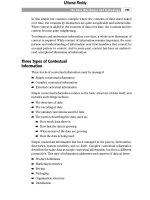
Figure 8.4 Normal probability plot of the WBC data in Example 8.1.
observations have the same value, the sample cumulative distribution function
is plotted against only the t with the largest i value.
Step 3. Plot t or a function of it versus the estimated sample cumulative
distribution or a function of it.
Step 4. Fit a straight line through the points by eye. The position of the
straight line should be chosen to provide a fit to the bulk of the data and may
ignore outliers or data points of doubtful validity.
Figure 8.4 gives a normal probability plot of the WBC versus \(F), where
\( · ) is the inverse of the standard normal distribution function. The values
of \(F (WBC
G
)) are shown in Table 8.1. The plot is reasonably linear. The
straight line fitted by eye in a probability plot can be used to estimate
percentiles and proportions within given limits in the same manner as for the
sample cumulative distribution curve. In addition, a probability plot provides
estimates of the parameters of the theoretical distribution chosen. The mean
(or median) WBC estimated from the normal probability plot in Figure 8.4 is
56,000 [at \(F) : 0, F : 0.5 and WBC: 56,000]. At \(F) : 1,
WBC : 91,000, which corresponds to the mean plus 1 standard deviation.
Thus, the standard deviation is estimated as 35,000.
We now discuss probability plots of the exponential, Weibull, lognormal,
and log-logistic distributions.
  203
Table 8.2 Probability Plotting for Example 8.2
Order, F,
ti(i 9 0.5)/21 log[1/(1 9 F)]
11
1 2 0.071 0.074
23
2 4 0.167 0.182

3 5 0.214 0.241
46
4 7 0.310 0.370
58
5 9 0.405 0.519
6 10 0.452 0.602
811
8 12 0.548 0.793
9 13 0.595 0.904
10 14
10 15 0.690 1.173
12 16 0.738 1.340
14 17 0.786 1.540
16 18 0.833 1.792
20 19 0.881 2.128
24 20 0.929 2.639
34 21 0.976 3.738
Exponential Distribution
The exponential cumulative distribution function is
F(t) : 1 9 exp[9(t)] t 9 0(8.2.1)
The probability plot for the exponential distribution is based on the relation-
ship between t and F(t), from (8.2.1),
t :
1

log
1
1 9 F(t)
(8.2.2)
This relationship is linear between t and the function log[1/(19 F(t))]. Thus,

an exponential probability plot is made by plotting the ith ordered observed
survival time t
G
versus log[1/(1 9 F (t
G
))], where F (t
G
) is an estimate of F(t
G
),
for example, (i 9 0.5)/n, for i : 1, , n.
From (8.2.2), at log+1/[1 9 F(t)], : 1, t : 1/. This fact can be used to
estimate 1/ and thus  from the fitted straight line. That is, the value t
204      
Figure 8.5 Exponential probability plot of the data in Example 8.2.
corresponding to log+1/[1 9F(t)], : 1 is an estimate of the mean 1/ and its
reciprocal is an estimate of the hazard rate .
Example 8.2 Suppose that 21 patients with acute leukemia have the
following remission times in months: 1, 1, 2, 2, 3, 4, 4, 5, 5, 6, 8, 8, 9, 10, 10, 12,
14, 16, 20, 24, and 34. We would like to know if the remission time follows the
exponential distribution. The ordered remission times t
G
and the log+1/
[1 9 F(t)], are given in Table 8.2. The exponential probability plot is shown
in Figure 8.5. A straight line is fitted to the points by eye, and the plot indicates
that the exponential distribution fits the data very well. At the point log[1/
(1 9 F(t))] : 1.0, the corresponding t, approximately 9.0 months, is an esti-
mate of the mean 1/ and thus an estimate of the hazard rate is  : 1/9 : 0.111
per month. An alternative is to use (7.2.5) to estimate ,  : 21/198: 0.107,
which is very close to the graphical estimate.

Weibull Distribution
The Weibull cumulative distribution function is
F(t) : 1 9 exp[9(t)A] t 90, 90, 90(8.2.3)
The probability plot for the Weibull distribution is based on the relationship
log t : log
1

;
1

log

log
1
1 9 F(t)

(8.2.4)
  205
between t and the cumulative distribution function F of t obtained from (8.2.3).
This relationship is linear between log t and the function log(log+1/[19F(t)],).
Thus, a Weibull probability plot is a graph of log(t
G
) and log(log+1/
[1 9 F (t
G
)],), where F (t
G
) is an estimate of F(t
G
), for example, (i 9 0.5)/n, for

i : 1, , n.
The shape parameter  is estimated graphically as the reciprocal of the slope
of the straight line fitted to the graph. If the fitted line is appropriate, then at
log(log+1/[1 9 F(t)],) : 0, the corresponding log(t) is an estimate of log(1/)
from (8.2.4). This fact can be used to estimate 1/ and thus  graphically from
a Weibull probability plot. At log(log+1/[1 9 F(t)],) : 0.5, (8.2.4) reduces to
log t : log(1/) ; 0.5/. This equation can be used to estimate .
Estimates of the parameters can also be obtained from the method described
in Chapter 7 if the Weibull distribution appears to be a good fit graphically.
The following hypothetical example illustrates the use of the Weibull probabil-
ity plot. The small number of observations used in the example is only for
illustrative purposes. In practice, many more observations are needed to
identify an appropriate theoretical model for the data.
Example 8.3 Six mice with brain tumors have survival times, in months of
3, 4, 5, 6, 8, and 10. Log(t
G
) plotted against log(log+1/[1 9 (i 9 0.5)/6],) for
i : 1, , 6 is shown in Figure 8.6. A straight line is fitted to the data point by
eye. From the fitted line, at log(log+1/[1 9 F(t)],) : 0, the corresponding
log(t) : 1.9, and thus an estimate of 1/ is approximately 6.69 [:exp(1.9)]
months and an estimate of  is 0.150. At log(log+1/[1 9 F(t)],) : 0.5, the
corresponding log(t) : 2.09, and thus an estimate of  : 0.5/(2.09—1.9) : 2.63.
The maximum likelihood estimates of  and  obtained from the SAS
procedure LIFEREG are 2.75 and 0.148, respectively. The graphical estimates
of  and  are close to the MLE.
Lognormal Distribution
If the survival time t follows a lognormal distribution with parameters  and
, log t follows the normal distribution with mean  and variance .
Consequently, (log t 9 )/ has the standard normal distribution. Thus, the
lognormal distribution function can be written as

F(t) : 

log t 9 


t 9 0(8.2.5)
where ( · ) is the standard normal distribution function and  and  are,
respectively, the mean and standard deviation of log t.
A probability plot for the lognormal distribution is based on the following
relationship obtained from (8.2.5):
log t :; \(F(t)) (8.2.6)
206      
Figure 8.6 Weibull probability plot of the data in Example 8.3.
The function \( · ) is the inverse of the standard normal distribution func-
tion or its 100F percentile. This relationship is linear between the value
log t and the function \(F(t)). Thus, a log-normal probability plot is a
graph of log(t
G
) versus \(F (t
G
)), where F (t
G
) is an estimate of F(t
G
).
From (8.2.6),at\(F(t)) : 0, log t : ; and at, \(F(t)) : 1, : log t 9 .
These facts can be used to estimate  and  from a straight line fitted to the
graph.
Example 8.4 In a study of a new insecticide, 20 insects are exposed.
Survival times in seconds are 3, 5, 6, 7, 8, 9, 10, 10, 12, 15, 15, 18, 19, 20, 22,

25, 28, 30, 40, and 60. Suppose that prior experience indicates that the survival
time follows a lognormal distribution; that is, some insects might react to the
insecticide very slowly and not die for a long time. The log(t
G
) versus
\[(i 9 0.5)/20], i : 1, , 20, are plotted in Figure 8.7. The plot shows a
reasonably straight line. From the fitted line, at \(F(t)) : 0, log t is an
estimate of , which is equal to 2.64, and at \(F(t)) : 1, log t : 3.4 and thus
 : 3.4 9 2.64 : 0.76. \(F(t)) can be obtained by applying Microsoft Excel
function NORMSINV.
  207
Figure 8.7 Lognormal probability plot of the data in Example 8.4.
Log-Logistic Distribution
The log-logistic distribution function is
F(t) :
tA
1 ; tA
t 9 0, 90, 90(8.2.7)
A probability plot for the log-logistic distribution is based on the following
relationship obtained from (8.2.7):
log t :
1

log

1
1 9 F(t)
9 1

9

1

log  (8.2.8)
Thus, a log-logistic probability plot is a graph of log(t
G
) versus log(+1/
[1 9 F (t
G
)], 9 1), where F (t
G
) is an estimate of F(t
G
), for example, (i 9 0.5)/n,
for i : 1, , n. From (8.2.8), at log+[1/(1 9 F)] 9 1, : 0, log t :9(1/) log ;
and at log+[1/(1 9F)] 9 1, :1, log t : (1/)(1 9 log ). These facts can be
used to estimate  and . The following example illustrates the log-logistic
probability plot.
Example 8.5 Consider the following survival times of 10 experimental rats
in days: 8, 15, 25, 30, 50, 90, 95, 100, 150, and 300. Figure 8.8 plots log(t
G
)
208      
Figure 8.8 Log-logistic probability plot of the data in Example 8.5.
against log(+1/[1 9 (i 9 0.5)/10], 9 1) for i : 1, , 10. To estimate  and ,
from the fitted line, at log(+1/[1 9 F(t)], 9 1) : 0, log t : 4.0; and at log(+1/
[1 9 F(t)], 9 1) : 1, log t : 4.6. Thus, we have two equations:
4.0 :9
1

log  and 4.6 :

1

(1 9 log)
From these two equations,  : 1.667 and  : 0.0013.
8.3 HAZARD PLOTTING
Hazard plotting (Nelson 1972, 1982) is analogous to probability plotting, the
principal difference being that the survival time (or a function of it) is plotted
against the cumulative hazard function (or a function of it) rather than the
distribution function. Hazard plotting is designed to handle censored data.
Similar to probability plotting, estimates of parameters in the distribution can
be determined from the hazard plot with little computational effort.
To determine if a set of survival time with censored observation is from a
given theoretical distribution, we construct a hazard plot by plotting the
survival time (or a function of it) versus an estimation cumulative hazard (or
  209
a function of it). The cumulative hazard function can be estimated by following
the steps below.
Step 1. Order the n observations in the sample from smallest to largest without
regard to whether they are censored. If some uncensored and censored
observations have the same value, they should be listed in random order. In
the list of ordered values, the censored data are each marked with a plus.
Step 2. Number the ordered observations in reverse order, with n assigned to
the smallest data value, n 9 1 to the second smallest, and so on. The numbers
so obtained are called K values or reverse-order numbers. For the uncensored
observation, K is the number of subjects still at risk at that time.
Step 3. Obtain the corresponding hazard value for each uncensored observa-
tion. Censored observations do not have a hazard value. The hazard value for
an uncensored observation is 1/K. This is the fraction of the K individuals who
survived that length of time and then failed. It is an observed conditional
failure probability for an uncensored observation.

Step 4. For each uncensored observation, calculate the cumulative hazard
value. This is the sum of the hazard values of the uncensored observation and
of all preceding uncensored observations. For tied uncensored observations,
the cumulative hazard is evaluated only at the smallest K among the uncen-
sored observations.
The table in the following example illustrates the procedure.
Example 8.6 Consider the remission data of the 21 leukemia patients
receiving 6-MP in Example 3.3. Table 8.3 illustrates the procedure for estima-
ting the cumulative hazard function.
We now discuss the basic idea underlying hazard plotting for the exponen-
tial, Weibull, lognormal, and log-logistic distributions.
Exponential Distribution
The exponential distribution has constant hazard function h(t) : . Thus, the
cumulative hazard function is
H(t) : t (8.3.1)
From (8.3.1), the time can be written as a linear function of the cumulative
hazard H,
t :
1

H(t)(8.3.2)
Thus, t plots as a straight-line function of H. The slope of the fitted line is the
210      
Table 8.3 Estimation of Cumulative Hazard
Reversed Cumulative
Order, Hazard, Hazard,
tK1/K H (t)
621 0.048
6; 20
619 0.053

618 0.056 0.156
717 0.059 0.215
9; 16
10 15 0.067 0.281
10; 14
11; 13
13 12 0.083 0.365
16 11 0.091 0.456
17; 10
19; 9
20; 8
22 7 0.143 0.598
23 6 0.167 0.765
25; 5
32; 4
32; 3
34; 2
35; 1
mean survival time 1/ of the distribution. More simply, 1/ is the value of t
when H(t) : 1. This fact is used to estimate 1/ from an exponential hazard
plot.
Example 8.7 Using the estimated cumulative hazard values H (t) in Table
8.3, we construct the exponential hazard plot in Figure 3.5 by plotting each
exact time t against its corresponding H (t). The configuration appears to be
reasonably linear, suggesting that the exponential distribution provides a
reasonable fit. In Chapter 3 we see that the Weibull distribution gives a better
fit than the exponential. We use the data here just to demonstrate how the
parameter can be estimated.
To find an estimate for the mean remission time of the leukemia patients,
we can use H(t) : 0.5 since the time for which H : 1 is out of the range of

the horizontal axis. At H(t) : 0.5, t : 16.9, from (8.3.2), an estimate of
 is 0.5/16.9: 0.0296. Thus, an estimate of the mean remission time is 34
weeks.
  211
Figure 8.9 Cumulative hazard functions of the Weibull distribution with :0.5, 1, 2, 4.
Weibull Distribution
The Weibull distribution has the hazard function
h(t) : (t)A\ t 9 0
The cumulative hazard function is
H(t) : (t)A t 90(8.3.3)
and is plotted in Figure 8.9 for four different values of : 0.5, 1, 2, and 4. From
(8.3.3), the time t can be written as a function of the cumulative hazard
function, that is,
t :
1

[H(t)]A (8.3.4)
Taking the logarithm of (8.3.4), we obtain
log t : log
1

;
1

log H(t)(8.3.5)
Since logt is a linear function of logH(t), a plot of log t against log H(t)isa
straight line. For log H(t) : 0orH(t) : 1, (8.3.5) reduces to log t : log(1/),
and thus the corresponding time t equals 1/. This fact is used to estimate 1/
and consequently, . The slope of the fitted straight line is 1/,orat
log H(t) : 1, (8.3.5) can be written as  : 1/(log t ; log). This equation can

be used to estimate .
212      
Figure 8.10 Weibull hazard plot of the data in Example 8.8.
Example 8.8 Consider the following survival times in months of 14
patients: 15, 25, 38, 40;, 50, 55, 65, 80;, 90, 140, 150;, 155, 250;, 252.
Figure 8.10 is the hazard plot with log t versus log H(t) of the data. From the
fitted line, at log H(t) : 0, log t : 4.8. Thus, t : 121.5 and the estimate of  is
 : 1/t : 0.0082. Similarly, at, log H(t) : 1, log t :5.6, and thus  : 1/
(5.6 9 4.8) : 1.25.
Lognormal Distribution
The density function of a lognormal distribution is
f (t) :
1
t(2
exp

9
1
2
(log t 9 )

:
1
t
g

log t 9 


t 9 0 (8.3.6)

where g(x) is the standard normal density function. The lognormal cumulative
distribution function is
F(t) : 

log t 9 


t 9 0(8.3.7)
  213
Figure 8.11 Cumulative hazard functions of the lognormal distribution with  :0.1,
0.5, 1.0.
where ( · ) is the standard normal distribution function. Thus, by (2.10), the
hazard function can be written as
h(t) :
1
t
g

log t 9 


1 9 

log t 9 


(8.3.8)
The cumulative hazard function, plotted in Figure 8.11 for three values of ,is
H(t) :9log


1 9 

log t 9


(8.3.9)
From (8.3.9), the logarithm of the survival time t as a function of the
cumulative hazard H is
log t : ; \[1 9 e\&R](8.3.10)
where \( ·) is the inverse of the standard normal distribution function.
Thus, log t is a linear function of \[19 e\&R]. The log-normal hazard
plot is a graph of log t versus \[1 9 e\&R]. From (8.3.10),at
\[1 9 e\&R] : 0, log t : ; and at \[1 9 e\&R] : 1, log t : ; .
These facts can be used to estimate  and .
Example 8.9 Consider the following remission times in months of 18
cancer patients: 4, 5, 6, 7, 8, 9;, 12, 12;, 13, 15, 18, 20, 25, 26;,28;, 35,
35;, 56. Figure 8.12 gives the log-normal hazard plot. From the fitted line by
eye, at \[1 9 e\&R] : 0, log t : 2.8; and at \[1 9 e\&R] : 1,
214      
Figure 8.12 Lognormal hazard plot of the data in Example 8.9.
log t : 3.76. Thus, the estimate of  is 2.8 and the estimate of  is
3.76 9 2.8: 0.96.
Log-Logistic Distribution
The cumulative hazard function of the log-logistic distribution is
H(t) : log(1 ; tA)
This equation can be written as
log t :
1

log+exp[H(t)] 9 1, 9

1

log  (8.3.11)
Thus, log t is a linear function of log+exp[H(t)] 9 1,. A log-logistic hazard plot
is a graph of log t versus log+exp[H(t)] 9 1,. From (8.3.11),at
log+exp[H(t)] 9 1, : 0, log t :9(1/) log ; and at log+exp[H(t)] 9 1, : 1,
log t : (1/) 9 (1/) log . These facts can be used to estimate  and .
8.4 COX SNELL RESIDUAL METHOD
The Cox—Snell (1968) residual method can be applied to any parametric
model. The Cox—Snell residual r
G
for the ith individual with observed survival
time t
G
, uncensored or censored, is defined as
r
G
:9logS (t
G
) i : 1, 2, , n (8.4.1)
—   215
where S (t) is the estimated survival function based on the MLE of the
parameters. If the observed t
G
is censored, the corresponding r
G
is also censored.
Since the cumulative hazard function H(t) :9log S(t), the Cox—Snell residual
r
G

is an estimated cumulated hazard value at t
G
. The important property of the
Cox—Snell residual is that if the model selected fits the data, r
G
’s follow the unit
exponential distribution with density function f
0
(r) : e\P.
Let S
0
(r) denote the survival function of the Cox—Snell residual r
G
. Then
S
0
: 

P
f
0
(x) dx : 

P
e\V dx : e\P, and
9log S
0
(r) :9log(e\P) : r (8.4.2)
Let S
0

(r) denote the Kaplan—Meier estimate of S
0
(r). It is clear from (8.4.2)
that the plot of r
G
versus 9log S
0
(r
G
) should be a straight line with unit slope
and zero intercept if the fitted survival distribution is appropriate, regardless
of the form of the distribution.
The procedure for using Cox—Snell residuals can be summarized as follows.
1. Use the methods shown in Sections 7.1 to 7.7 to find the MLE of the
parameters of the selected theoretical distribution.
2. Calculate Cox—Snell residuals r
G
:9log S (t
G
), i : 1, 2, , n, where S (t
G
)
is the estimated survival function with the MLE of the parameters.
3. Apply the Kaplan—Meier method to estimate the survival function S
0
(r)
of the Cox—Snell residuals r
G
’s obtained in step 2, then using the estimate
S

0
(r), calculate 9log S
0
(r
G
), i : 1, 2, , n.
4. Plot r
G
versus 9log S
0
(r
G
), i : 1, 2, , n. If the plot is closed to a straight
line with unit slope and zero intercept, the fitted distribution is appropri-
ate.
From (8.4.1), if an individual survival time is right-censored, say, t
>
G
and
the fitted model is correct, the corresponding Cox—Snell residual
9log S(t
>
G
) : H(t
>
G
) is smaller than the residual evaluated at an uncensored
observation with the same value t
G
since H(t) is a monotone-increasing function

of t. To take this into account, two modified Cox—Snell residuals have been
proposed for censored observations (Crowley and Hu, 1977). One is based on
the mean, and the other is based on the median (:log 2 : 0.693) of the unit
exponential distribution by assuming that difference between H(t
G
) and H(t
>
G
)
also follows the unit exponential distribution. For a censored observation t
>
G
,
the modified residual r
>
G
is defined as
r
>
G
: r
G
; 1(8.4.3)
or
r
>
G
: r
G
; 0.693 where r

G
:9logS (t
G
)(8.4.4)
Example 8.10 Consider the tumor-free time data observed from rats fed
with saturated diets in Table 3.4. We select the lognormal distribution for this
216      
Figure 8.13 Cox—Snell residual plot for the fitted lognormal model on the tumor-free
time data for rats fed with saturated diets.
set of data for illustrative purposes. Using methods discussed in Chapter 7, the
MLE of the parameters obtained are : 4.76458 and  : 0.56053. We then
calculate the Cox—Snell residuals r
G
:9log S(t
G
) :9log[1 9 F(t
G
)], where
F(t) is the distribution function of the lognormal distribution. An easy way to
compute r
G
for the lognormal distribution is to use the relationship between the
normal and lognormal distributions, i.e., the distribution function of the
lognormal distribution, F(t), is equivalent to [(log t 9 )/], where ()is the
distribution function of the standard normal distribution. We can use Micro-
soft Excel function NORMSDIST to calculate (t). Thus, for the lognormal
distribution,
S(t
G
) : 1 9 ([log(t

G
) 9 4.76458]/0.56053)
Using the specific notation of NORMSDIST, ln for log,
r
G
:9ln(1 9 normsdist+[ln(t
G
) 9 4.76458]/0.56053,)
The r
G
’s so obtained are given in Table 8.4. The next step is to obtain the
Kaplan—Meier estimate of the survival function S(r
G
), and compute 9log S(r
G
).
These values are also given in Table 8.4.
Figure 8.13 gives the graph of r
G
versus 9logS
0
(r
G
), i : 1, , 22. The graph
is close to a straight line with unit slope and zero intercept. Therefore, a
—   217
Table 8.4 Kaplan Meier Estimate of Survivorship
Function for the Cox Snell Residuals from the Fitted
Lognormal Model on Tumor-Free Time Data for Rats
Fed with Saturated Diets

tr? S
0
(r)@ 9log S
0
(r)
0.000 1.000 0.000
43 0.037 0.967 0.034
46 0.049 0.933 0.069
56 0.098 0.900 0.105
58 0.110 0.867 0.143
68 0.181 0.833 0.182
75 0.239 0.800 0.223
79 0.275 0.767 0.266
81 0.294 0.733 0.310
86 0.342 0.667 0.405
86 0.342 0.667 0.405
89 0.373 0.633 0.457
96 0.447 0.600 0.511
98 0.469 0.567 0.568
105 0.548 0.533 0.629
107 0.571 0.500 0.693
110 0.606 0.467 0.762
117 0.690 0.433 0.836
124 0.776 0.400 0.916
126 0.800 0.367 1.003
133 0.889 0.333 1.099
142 1.004 0.267 1.322
142 1.004 0.267 1.322
165 1.305 0.233 1.455
170; 1.371;

200; 1.769;
200; 1.769;
200; 1.769;
200; 1.769;
200; 1.769;
200; 1.769;
? r, ordered Cox—Snell residuals from the fitted lognormal model.
@S
0
(r), Kaplan—Meier estimate of survivorship function for the
Cox—Snell residuals.
lognormal model may be appropriate for the tumor-free times observed. In
Chapter 9 (Example 9.2) we will see that the lognormal model was not rejected
based on a goodness-of-fit test. Thus the result is consistent with those
obtained by using the analytical method. A weakness of the Cox—Snell residual
method is that the plot does not indicate the kind of departure the data have
from the model selected if the configuration is not linear.
218      
Bibliographical Remarks
Probability plotting has been widely used since Daniel’s (1959) classical work
on the use of half-normal plot. A quite complete and excellent treatment of
probability plotting is given by King (1971). Although examples given are
applications to industrial reliability, its interpretation of probability plots of
many distributions, such as the uniform, lognormal, Weibull, and gamma, are
applicable to biomedical research. Recent applications of probability plotting
include Leitner et al. (1986), Horner (1987), Waters et al. (1991), and
Tsumagari et al. (2000).
Hazard plotting was developed by Nelson (1972, 1982). Applications in-
cluded Gore (1983) and Wurpel et al. (1986).
EXERCISES

8.1 Show that the Cox—Snell residuals defined in (8.4.1) follow the unit
exponential distribution with density function f (r) : exp(9r).
8.2 Consider the following survival times of 16 patients in weeks: 4, 20, 22,
25, 38, 38, 40, 44, 56, 83, 89, 98, 110, 138, 145, and 27.
(a) Does the exponential distribution provide a reasonable fit to the
survival data? Use the probability plotting technique.
(b) Estimate graphically the parameter  of the exponential distribution
and consequently, the mean survival time.
8.3 To computerize patients’ records, a data clerk is hired to transcribe
medical data from the patients’ charts to computer coding forms. The
number of correct entries between errors is listed in chronological order
of occurrence over a period of five days as follows: 73, 12, 40, 65, 100,
15, 70, 40, 110, 64, 200, 6, 90, 102, 20, 102, 90, 34. The assumption is that
the data clerk, during the five days, would not change her error rate
appreciably. Use the technique of probability plotting to evaluate the
assumption above. What is your conclusion?
8.4 Twenty-five rats were injected with a give tumor inoculum. Their times,
in days, to the development of a tumor of a certain size are given below.
30 53 77 91 118
38 54 78 95 120
45 58 81 101 125
46 66 84 108 134
50 69 85 115 135
Which of the distributions discussed in this chapter provide a reasonable
fit to the data? Estimate graphically the parameters of the distribution
chosen.
 219
8.5 In a clinical study, 28 patients with cancer of the head and neck did not
respond to chemotherapy. Their survival times in weeks are given below.
1.7 8.3 14.0 22.7 6.0; 13.1;

5.1 9.6 15.9 33.0 7.4; 13.4;
5.3 11.3 16.7 3.7; 8.0; 16.1;
6.0 12.1 17.0 5.0; 8.3;
8.3 12.3 21.0 5.9; 9.1;
(a) Make a hazard plot for each of the following distributions: exponen-
tial, Weibull, lognormal, and log-logistic.
(b) Which distribution provides a reasonable fit to the data? Estimate
graphically the parameters of the distribution chosen.
8.6 Thirty-one patients with advanced melanoma treated with combined
chemotherapy, immunotherapy, and hormonal therapy have survival
times as given below.
26.3; 16.1 24.0 4.3 31.3;
94.0 49.6 77.9 97.6; 17.6;
9.1 27.3 16.6; 7.3 16.3
34.6; 61.9; 3.4 75.6;
9.4 46.6; 10.9 14.3
25.7 22.4; 13.0 56.4
88.7 7.1 64.4; 9.1
(a) Make a hazard plot for each of the following distributions: exponen-
tial, Weibull, lognormal, and log-logistic.
(b) Which distribution provides a reasonable fit to the data? Estimate
the parameters of the distribution chosen.
8.7 Consider the survival times of the hypernephroma patients in Exercise
Table 3.1 (see Exercise 4.5). Make a hazard plot for the distribution you
chose in Exercise 6.8. Did you make a good selection? If not, try two
other distributions.
8.8 Consider the following survival times in weeks of 10 mice with injection
of tumor cells: 5, 16, 18;, 20, 22;,24;, 25, 30;, 35, 40;. Make an
exponential hazard plot. Does the exponential distribution provide a
reasonable fit? If not, is the lognormal distribution better?

8.9 Consider the following survival times in months of 25 patients with
cancer of the prostate. Use a graphical method to see if the survival time
of prostate cancer patients follows the exponential distribution with
 : 0.01: 2, 19, 19, 25, 30, 35, 40, 45, 45, 48, 60, 62, 69, 89, 90, 110, 145,
160, 9;,10;,20;,40;,50;, 110;, 130;.
8.10 Make a log-logistic hazard plot of the following data and estimate the
two parameters: 20, 30, 32;, 40, 60, 100, 150, 200;, 300.
220      
CHAPTER 9
Tests of Goodness of Fit
and Distribution Selection
In Chapter 8 we discuss three graphical methods for checking if a parametric
distribution fits the observed data. Parametric distributions can be grouped
into families. First, any given distribution with different parameter values forms
a family. Second, if a distribution includes other distributions as its special
cases, this distribution is a nesting (larger) family of these distributions. For
example, the distributions introduced in Chapter 6 belong to more than one
nested family. First, the Weibull distribution reduces to the exponential when
 : 1. Therefore, the exponential distribution is a special case of the Weibull
and the two distributions are said to belong to one family, the Weibull family.
Second, consider the standard gamma distribution; when : 1, it reduces to
the exponential, and when  :


and  :


, it becomes the chi-square
distribution with  degrees of freedom. Thus, the gamma distribution includes
the exponential and chi-square as a family. Now let us consider the generalized

gamma distribution. It reduces to the exponential if  : : 1, the Weibull if
 : 1, the lognormal if  ; -, and the gamma if  : 1. Thus, the generalized
gamma distribution includes these four distributions and represents a large
family of distributions. The relationship of the generalized gamma distribution
to the exponential, Weibull, lognormal, and gamma distributions allows us to
evaluate the appropriateness of these distributions relative to each other and
to a more general distribution. It is known that the generalized gamma
distribution is a special case of the generalized F-distribution and therefore
belongs to the generalized F family (Kalbfleisch and Prentice, 1980) Because
of its complexity, we do not cover the generalized F family.
In this chapter we discuss several analytical procedures for comparing
parametric distributions and assessing goodness of fit. In Section 9.1 we
introduce several widely used statistics for testing the appropriateness of a
distribution. Readers who are not familiar with linear algebra or are not
interested in the mathematical details may skip this section without loss of
continuity. In Section 9.2 we discuss statistics for testing whether a distribution
221
is appropriate by comparing it with other distributions in the same family or
a more general family. Section 9.3 covers the selection of a distribution based
on Baysian information criteria. Section 9.4 covers the statistics for testing
whether a given distribution with known parameters is appropriate. All the test
statistics discussed in Sections 9.1 to 9.4 are based on asymptotic likelihood
inferences. In Section 9.5 we introduce the test statistic of Hollander and
Proschan (1979) for testing whether a distribution with given parameters is
appropriate. Computer codes for BMDP or SAS that can be used to carry out
the test procedures are provided.
9.1 GOODNESS-OF-FIT TEST STATISTICS BASED ON
ASYMPTOTIC LIKELIHOOD INFERENCES
We take the exponential distribution as an example to see how to construct
statistics to test whether it is appropriate for the observed survival times. As

noted in Chapter 6, the Weibull family with  : 1, the gamma family with
 : 1, and the generalized gamma family with  : : 1 reduce to the
exponential distribution. Therefore, to test if the exponential distribution is
appropriate for the observed survival time, we can first fit a Weibull distribu-
tion and test if  : 1, or fit a gamma distribution, then test if  : 1, or fit a
generalized gamma distribution, then test if :  : 1. Similarly, to test
whether the family of Weibull distributions, or the gamma distributions, or the
lognormal distributions is appropriate for the survival data observed, we can
fit a generalized gamma distribution (their nesting distribution) and then test
if  :1, or  : 1, or with  ; -, respectively. Thus, testing the appropriateness
of a family of distributions is equivalent to testing whether a subset of the
parameters in its nesting distribution equal to some specific values. If the data
can be assumed to follow a certain distribution but the values of its parameters
are uncertain, we need to test only that the parameters are equal to certain
values. In the following, we separately introduce test statistics for testing
whether some of the parameters in a distribution are equal to certain values
and whether all parameters in a distribution are equal to certain values.
Readers who are interested in a detailed discussion of these statistics are
referred to Kalbfleisch and Prentice (1980).
9.1.1 Testing a Subset of Parameters in a Distribution
Let b : (b

, b

) denote all the parameters in a parametric distribution, where
b

and b

are subsets of parameters, and let the hypothesis be

H

: b

: b

(9.1.1)
where b

is a vector of specific numbers. Let b be the MLE of b, b

(b

) the
MLE of b

given b

: b

, and V

(b ) the submatrix of the covariance matrix in
222        
(7.1.5), V (b ), corresponding to b

. Under H

and some mild assumptions, both
of the following two statistics have an asymptotic chi-square distribution with

degrees of freedom equal to the dimension of (or the number of parameters in)
b

.
Log-likelihood ratio statistic:
X
*
: 2[l(b ) 9 l(b

(b

), b

)] (9.1.2)
Wald statistic:
X
5
: (b

9 b

)V
\

(b )(b

9 b

)(9.1.3)
If the number of parameters in b


is equal to q, for a given significant level
, H

is rejected if X
*
9

O?
when the likelihood ratio statistic is used; or if
X
5
9

O?
or X
5
:

O\?
, (two-sided test) or X
5
9

O?
(one-sided test)
when the Wald’s statistic is used, where 

O?
, 


O?
and 

O\?
are the
100(1 9 ), 100(1 9/2), and 100/2 percentile points of the chi-square dis-
tribution with q degrees of freedom; that is,
P(

O
9

O?
) :  and P(

O
9

O?
) : P(

O
:

O\?
) :

2
Example 9.1 Suppose that we wish to test whether the observed data are

from an exponential distribution. We can use a Weibull distribution and test
whether its shape parameter, , is equal to 1. The Weibull distribution has two
parameters,  and ; thus b : (, ) and the null and alternative hypotheses are:
H

:  : 1 (the underlying distribution is an exponential distribution)
(9.1.4)
H

:  "1 (the underlying distribution is a Weibull distribution)
Let b : ( ,  ) be the MLE of b, l
5
(b ) : l
5
( ,  ) and l
#
( ) be the log-likelihood
of the Weibull and exponential distributions, respectively, l
#
( ) Y l
5
( (1),1),
where  (1) is the MLE of  in the Weibull distribution given  : 1. The
log-likelihood ratio and Wald statistics defined in (9.1.2) and (9.1.3) in this case
become
X
*
: 2[l
5
( ,  ) 9 l

5
( (1),1)] (9.1.5)
and
X
5
: ( 9 1)V

\

( ,  )( 9 1) (9.1.6)
--   223
respectively, where V

( ,  ) is the second diagonal element of the covariance
matrix
V ( ,  ) :9

*l
5
( ,  )
*
*l
5
( ,  )
* *
*l
5
( ,  )
* *
*l

5
( ,  )
*

\
(9.1.7)
and
V
\

( ,  ) :9
[*l
5
( ,  )/*][*l
5
( ,  )/*] 9 (*l
5
( ,  )/* *)
*l
5
( ,  )/*
(9.1.8)
For a given significant-level , H

is rejected if X
*
9

?
, when the likelihood

ratio statistic is used; or if X
5
9

?
or X
5
:

\?
, when the Wald
statistic is used.
It must be pointed out that failure to reject H

in (9.1.4) does not imply that
an exponential distribution provides the best fit to the data. On the other hand,
rejection of H

does not indicate that a Weibull distribution is the choice
either. Further testing of other distributions is needed. The details and
examples are given in Section 9.2.
Since the gamma and generalized gamma distribution also include the
exponential as a special case, similar test statistics can be constructed to test
the null hypothesis that the data are from the exponential distribution by using
the gamma, the generalized gamma, or the extended generalized gamma
distribution.
9.1.2 Testing All Parameters in a Distribution
To test whether all of the parameters in b equal a given set of known values
b


, the null hypothesis is
H

: b : b

(9.1.9)
and the following three test statistics can be used.
Log-likelihood ratio statistic:
X
*
: 2[l(b ) 9 l(b

)] (9.1.10)
Wald statistic:
X
5
:9(b 9 b

)
*l(b

)
*b *b
(b 9 b

)

or :9(b 9 b

)

*l(b )
*b *b
(b 9 b

)

(9.1.11)
224        
Score statistic:
X
1
:

*l(b

)
*b



9
*l(b

)
*b *b

\ *l(b

)
*b


or :

*l(b

)
*b


V (b )
*l(b

)
*b

(9.1.12)
where V (b ) is the estimated covariance matrix in (7.1.5). Under H

and the
assumption that b has approximately multinormal distribution, each of the
three statistics has an asymptotic chi-square distribution with p (the dimension
of b or the number of parameters in b) degrees of freedom.
For a given significant-level , H

is rejected if X
*
9

N?
, when the

likelihood ratio statistic is used; or if X
5
9

N?
or X
5
:

N\?
, when the
Wald statistic is used; or if X
1
9

N?
or X
1
:

N\?
, when the score statistic
is used.
It must be pointed out that rejection of H

in (9.1.9) means only that the
given distribution with the known parameters b

, not the family of distribu-
tions to which the given distribution belongs, is not appropriate for the

observed data. It is possible that a distribution with different b

in the family
may be appropriate.
9.2 TESTS FOR APPROPRIATENESS OF A FAMILY OF
DISTRIBUTIONS
The usual method for testing whether a distribution is appropriate for the
observed data is to compare the distribution with a larger or more general
family that includes the distribution of interest as a special case (Hagar and
Bain, 1970).
Let l
#
(), l
5
(, ), l
%
(, ), l
*,
(, ), and l
%%
(, , ) denote, respectively,
the log-likelihood function defined in (7.1.1) based on the exponential, Weibull,
gamma, lognormal, and extended generalized gamma distribution, and l
#
( ),
l
5
( ,  ), l
%
( ,  ), l

*,
( ,  ), and l
%%
( ,  ,  ) denote the respective log-likelihood
values where  , ( ,  ), ( ,  ), ( ,  ), and ( ,  ,  ) are the MLE. For example, the
log-likelihood of the exponential distribution can be obtained from
l
#
( ) :
P

G
log( e
9 t
G
) ;
L

GP>
log(e
9t
>
G
) : r log  9 
P

G
t
G
9 

L

GP>
t
>
G
for a set of observed survival times t

, , t
P
, t
>
P>
, , t
>
L
. The log-likelihood
value and the estimated covariance matrix in (7.1.5) and parameters for each
of the distributions discussed in Sections 7.2 to 7.6 can be obtained from SAS
or BMDP. The results can be used to construct the log-likelihood ratio statistic
and the Wald statistic defined in (9.1.2) and (9.1.3). In the following, we
        225
introduce several tests for the appropriateness of a family of distributions based
on the log-likelihoods. Construction of the respective Wald statistics is left to
the reader as exercises.
1. Testing the hypothesis that the underlying distribution is exponential. The
null hypothesis is
H

: The underlying distribution is an exponential distribution

If the Weibull distribution is used, testing the null hypothesis above is
equivalent to testing the following null and alternative hypotheses:
H

:  : 1 (the underlying distribution is an exponential distribution)
H

:  "1 (the underlying distribution is a Weibull distribution)
Let  (1) be the MLE of  in the Weibull distribution given  : 1, the
log-likelihood ratio statistic is
X
*
: 2[l
5
( ,  ) 9 l
5
( (1),1)] (9.2.1)
which has an asymptotic chi-square distribution with 1 degree of freedom. For
a given level of significance , H

is rejected if X
*
9

?
. Note that
l
5
( (1),1) Y l
#

( ).
Similarly, a log-likelihood ratio statistic can be constructed by using the
gamma or the extended generalized gamma distribution. These will be left to
the reader as exercises.
2. Testing the hypothesis that the underlying distribution is Weibull. The null
hypothesis is
H

: The underlying distribution is a Weibull distribution
We can use the extended generalized gamma distribution and test whether its
parameter  equals 1. Thus the null and alternative hypotheses can be stated as
H

:  : 1 (the underlying distribution is a Weibull distribution)
H

:  "1 (the underlying distribution is an extended generalized
gamma distribution)
Let  (1) and  (1) be the MLE of  and  in the extended generalized gamma
distribution given : 1. According to Section 6.4, an extended generalized
226        
gamma distribution with : 1 is a Weibull distribution. The likelihood ratio
statistic is
X
*
: 2[l
%%
( ,  ,  ) 9 l
%%
( (1),  (1), 1)] (9.2.2)

which follows asymptotically the chi-square distribution with 1 degree of
freedom. H

is rejected at a significance level of  if X
*
9

?
. Note that
l
%%
( (1),  (1), 1) Y l
5
( ,  ).
3. Testing the hypothesis that the underlying distribution is standard gamma.
The null hypothesis is
H

: The underlying distribution is a gamma distribution
Following the same logic in Section 6.4, the null hypothesis above is equivalent
to the following if the extended generalized gamma distribution is used.
H

:  : 1 (the underlying distribution is a standard gamma distribution)
H

:  "1 (the underlying distribution is a generalized gamma distribution).
The likelihood test statistic is
X
*

: 2[l
%%
( ,  ,  ) 9 l
%%
(1,  (1),  (1))] (9.2.3)
where  (1) and  (1) are the MLE of  and  given  : 1, which has an
asymptotic chi-square distribution with 1 degree of freedom under H

. The
rejection rule is the same as that for the exponential or Weibull distribution.
Note that l
%%
(1,  (1),  (1)) Y l
%
( ,  ).
4. Testing the hypothesis that the underlying distribution is lognormal. The
null hypothesis is
H

: the underlying distribution is a lognormal distribution
The log-likelihood test statistic is
X
*
: 2[l
%%
( ,  ,  ) 9 l
*,
( ,  )]
which has an asymptotic chi-square distribution with 1 degree of freedom
under H


. The rejection rule is the same as that for the exponential or Weibull
distribution.
For the log-logistic and extended generalized gamma distributions, it can be
shown that a generalized F-distribution (Kalbfleisch and Prentice, 1980)
includes the exponential, Weibull, lognormal, gamma, generalized gamma,
        227